Incorporating inherent variability into numerical simulations of velocity effects: a behavior-based CPTu study on gold tailings

Abstract

This study presents a detailed characterization of the inherent variability of a silty gold tailings deposit on the basis of piezocone penetration test (CPTu) data. The database originates from a comprehensive site investigation campaign and was processed via a layer separation algorithm to identify strata and determine relevant statistical parameters. Profiles were classified considering granular (drained), intermediate (partially drained), and fine (undrained) material behavior, allowing for behavior-specific probabilistic analysis of cone resistance (q_c), sleeve friction (f_s), and pore pressure (u₂). The results revealed greater measurement variability for q_c, f_s, and u₂ in coarse-grained materials, whereas the strength parameters—particularly the undrained shear strength (Su)—exhibit greater variability in fine-grained materials. The classification approach also enabled a consistent estimation of the scale of fluctuation, an essential parameter for spatial variability modeling. A complementary numerical analysis illustrated the influence of inherent variability on the normalized cone resistance (q_c/q_cUD) under different drainage conditions. Greater dispersion occurred at lower velocities, which is characteristic of drained behavior. The alignment between the theoretical bounds and field data supports the robustness of the methodology, providing a valuable framework for reliability-based geotechnical design.

Keywords
Inherent variability; Spatial variability; Partial drainage

1. Introduction

Probabilistic analyses are indispensable for effectively managing risks and supporting the design and maintenance of geotechnical structures. These approaches have been applied in a wide range of scenarios, including foundation systems, embankments, slopes, and tailings dams (Phoon et al., 2022).

A key challenge in probabilistic modeling is the high data density required for reliable statistical characterization. Conventional site investigations are often constrained by cost and logistics, resulting in sparse data. In this context, the piezocone penetration test (CPTu) has emerged as a valuable tool, providing continuous measurements along a vertical profile and thus enabling the extraction of large, high-resolution datasets. As noted by Salgado et al. (2015), such datasets reduce the potential for bias and enable robust statistical and probabilistic analyses.

Recent studies have highlighted the reliability of CPT (cone) and CPTu (piezocone) data in estimating key spatial variability descriptors, including the coefficient of variation (COV), probability density function (PDF), and vertical scale of fluctuation (δv). For example, Pieczyńska-Kozłowska et al. (2021) compared fluctuation scales calculated from CPT and CPTu data in natural clays. Their results confirmed the consistency of the use of direct measurements (q_c and f_s) and derived parameters such as the friction angle, cohesion, and undrained shear strength.

Hu & Wang (2024) proposed a method to assess profile homogeneity on the basis of autocorrelation functions, comparing original CPT profiles with partial segments. Although effective, their method requires careful preprocessing, including detrending and segmentation, before residuals can be used to generate representative random fields.

Agbaje et al. (2024) employed random field modeling to investigate the failure behavior of a cut slope in clay, interpreting the undrained shear strength from ten CPTu profiles. Using a log-normal distribution and Bayesian calibration, they established consistent probabilistic fields. Their findings suggested that failure probabilities were not significantly affected by fluctuations in correlation length. However, they also highlighted persistent challenges in characterizing variability across material transitions, such as from clays to sands, which induce spikes in autocorrelation and complicate the estimation of correlation lengths.

In the context of silty materials (mainly tailings), Becker et al. (2024), Dienstmann et al. (2025a, b), and Campos et al. (2025) can be cited. Becker et al. (2024) assessed the variability of undrained shear strength in iron tailings from the Germano dam and reported that the normalized strength Su/σ′_vt followed a lognormal distribution and that thicker plastic layers exhibited lower mean values and reduced variability. In the applications presented by Dienstmann et al. (2025a, b), the objective was to characterize the variability of a gold tailings deposit through the analysis of individual CPTu sounding profiles, seeking to establish behavioral patterns, variations in COV, and the most recurrent PDFs for modeling parameters such as q_c, f_s, and u₂. The material exhibited high variability, with COV values ranging from 0.18-5.27 (18-527%). Some soundings also presented greater difficulty in defining PDFs. The lognormal distribution appeared to be a suitable fit for modeling the variability of the q_c and f_s data, whereas a normal distribution was more appropriate for modeling the u₂ data. In some cases, the exponential distribution provides an adequate fit for certain parameters at specific soundings. Fluctuation scales were also addressed in Dienstmann et al. (2025a), evaluated by individual sounding profiles, and were found to range from 0.10-2.04 m.

Expanding on this research, Campos et al. (2025) characterized the spatial variability of bauxite tailings using CPTu data, evaluated vertical fluctuation scales (δv) through theoretical autocorrelation model fitting, along with PDF estimation and stationarity analysis of the profiles. Their work also introduced a classification scheme (based on the Soil Behavior Index Ic_RW) to separate profiles into drained, partially drained, and undrained categories. The basic statistical characterization was performed after careful separation of profile segments and removal of trends, followed by grouping according to the material’s behavioral characteristics. This approach proved more appropriate for analyzing the variability of the f_s, q_c, and u₂ readings, as well as the derived parameters.

The present study builds upon the approach proposed by Dienstmann et al. (2025a, b) by integrating the classification algorithm developed by Campos et al. (2025) to separate the dataset according to drainage behavior in combination with an independently developed trend analysis. This stratification enables the statistical characterization of granular (drained), intermediate (partially drained), and fine (undrained) material behavior. On the basis of this classification, the most appropriate probability density functions (PDFs) for each behavioral classification were identified, providing a statistical basis for subsequent numerical modeling.

2. Theoretical background

2.1 Random field theory

Inherent variability in geotechnical parameters can be discretized through the spatial representation of random fields, as described by Phoon & Kulhawy (1999). In this framework, a geotechnical parameter can be expressed as a combination of two components: a deterministic trend component—typically depth dependent—and a fluctuation component representing local variability or noise, as shown in Equation 1:

$$\xi (x)=t(x)+w(x)$$ (1)

where ξ(x) is the geotechnical parameter under consideration, t(x) represents the deterministic trend, and w(x) denotes the fluctuation or residual component.

The fluctuation term w(x) can be characterized using basic statistical descriptors such as the mean (μ), standard deviation (σ), probability distribution function (e.g., Normal, Lognormal), and spatial correlation structure. The latter is typically described using the spatial correlation length (SCL, which is also denoted as δ, or scale of fluctuation, SOF), a concept first introduced by Vanmarcke (1977). Together with the autocorrelation function, the SOF defines how a property is spatially correlated.

Since its introduction by Vanmarcke (1977), the concept of the SOF has been widely discussed, with several methodologies proposed for its estimation (e.g., Kenarsari et al., 2013; Nie et al., 2015; Salgado et al., 2015). The theoretical autocorrelation model adjustment (TAM) was used in the present study and will be briefly described.

2.2 Autocorrelation function

The autocorrelation function itself is a statistical measure that reflects the degree of similarity between data points as a function of their spatial separation. It is computed in two steps:

1. Covariance calculation between values of a variable X at points separated by a lag τ_j ​ (Equation 2);

2. Normalization of this covariance by the variance of the data (Equation 3) yields the sample autocorrelation ρ(τ_j​).

The lag τ_j is defined in Equation 4:

$C\left({\tau }_j\right)=\frac{1}{n}{{\displaystyle \sum }}_{i=1}^{n-j}\left(X_i-{\mu }_X\right)\left(X_{i+j}-{\mu }_X\right)$ (2)

$\rho \left({\tau }_j\right)=\frac{C\left({\tau }_j\right)}{C\left({\tau }_1\right)}$ (3)

${\tau }_j=\left(j-1\right)\Delta z$ (4)

where: $C\left({\tau }_j\right)=\text{covariance}$ at lag${\tau }_j$; $n=\text{number of available measurements}$; $X_i=\text{value of the parameter}X\text{at depth}{z}_i$; ${\mu }_X=\text{mean of}X$; $j=\text{index for lag steps}$; $\rho \left({\tau }_j\right)=$ sample autocorrelation; $C\left({\tau }_1\right)=$ variance (covariance at zero lag); $\Delta z=\text{minimum spacing between measurements}$; and ${\tau }_j=\text{separation distance between points}{X}_i\text{and}{X}_{i+j}.$

After defining the autocorrelation function from field data, numerical models can be applied to estimate the scale of fluctuation using the TAM method. In this approach, the vertical spatial correlation length is obtained by fitting theoretical autocorrelation functions to the empirically derived autocorrelation. Table 1 summarizes the most common theoretical models and their corresponding relationships between the separation distance (τ) and the scale of fluctuation (δ).

Table 1
TAM models.

TAM	Autocorrelation function
Exponential	$\rho \left(\tau \right)=exp\left(-\frac{2\left|\tau \right|}{\delta }\right)$
Squared Exponential	$\rho \left(\tau \right)=exp\left(-\pi {\left(\frac{\tau }{\delta }\right)}^2\right)$
Exponential Cosine	$\rho \left(\tau \right)=\cos \left(\frac{\tau }{\delta }\right)exp\left(-\frac{\left|\tau \right|}{\delta }\right)$
Second Order Markov	$\rho \left(\tau \right)=\left(1+\frac{4\left|\tau \right|}{\delta }\right)exp\left(-\frac{4\left|\tau \right|}{\delta }\right)$

2.3 Important considerations for estimating SOF

Several practical considerations influence the accuracy and interpretation of SOF values:

1. Soil stratification significantly affects SOF estimation (Overgård, 2015);

2. The sample resolution is critical—a spacing smaller than 1/5-1/4 of the SOF is recommended for reliability (Huber, 2013);

3. The soil type, test method, and location all impact spatial correlation behavior (Uzielli et al., 2007).

Larger SOF values indicate smoother spatial variations and stronger correlations between nearby data points, whereas smaller values suggest abrupt changes and weaker spatial correlations. Extending the concepts described above to tailings requires careful consideration of trend variability. Direct comparisons of piezocone tests from different investigation islands within the same tailings storage facility (TSF) can reveal distinct behavioral patterns, as reported by Dienstmann et al. (2018a), which must be accounted for in the analysis.

3. Materials and methods

3.1 Site characterization – gold tailings

The tailings storage facility (TSF) of the Fazenda Brasileiro Mine has been the focus of a research project aimed at understanding the geomechanical behavior of tailings (Schnaid et al., 2020). The investigation involved field and laboratory testing, covering eleven investigation islands. Field tests included piezocone tests (CPTu and SCPTu), seismic dilatometer tests (SDMTs), and vane shear tests. The laboratory results revealed predominantly silty sand with low to nonplastic behavior, high specific gravity (Gs between 2.79 and 3.30 g/cm³), an average solid content of ~30%, and a water content of approximately 35%. Triaxial tests under monotonic loading defined a critical state friction angle near 30°.

Standard CPTu tests (20 mm/s) and variable penetration rate tests have been used to assess drainage behavior (Schnaid et al., 2016; Dienstmann et al., 2017, 2018a, 2025a). Variability analysis for this material was recently introduced by Dienstmann et al. (2025a, b). In this study, only standard-rate CPTu results are considered for inherent variability assessment. The analyzed database includes tests from multiple campaigns—PZC01–PZC08 (Bedin, 2010), I1K and I2K (Klahold, 2013), and I1S (Sosnoski, 2016). The vertical spatial variability is evaluated via the cone resistance (q_c), sleeve friction (f_s), pore pressure (u₂), and derived resistance parameters. Two typical behaviors identified by Dienstmann et al. (2018a) (Figure 1) are used as a reference:

Figure 1
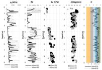
Piezocone profile friction angle (ϕ) and undrained strength (Su) interpretation (Dienstmann et al., 2025b).

• Coarse material (PZC02, PZC03, PZC05), in the central area (elev. ~359 m), with high q_c, low u₂ and f_s, and a shallow water table (~7 m);

• Fine material (e.g., PZC01, PZC04, PZC06–08, IK01–02, IS01), in peripheral zones (elev. 352–356 m), resulting in a lower q_c, higher u₂ and B_q, and greater f_s.

These patterns reflect depositional processes, where coarser particles settle earlier during transport, whereas finer sediments accumulate further from the discharge point. Although such separation by the depositional process can be considered, the statistical analysis described in Section 3 introduces a refined evaluation of the material’s behavior by segmenting portions of the same profile according to their response. This behavioral classification was also considered for the derivation of parameters such as the friction angle (ϕ′) and undrained shear strength (Su).

For friction angle determination, Kulhawy & Mayne (1990), Mayne & Campanella (2005), and the Norwegian University of Science and Technology (NTNU) method (Senneset et al., 1988; 1989) were considered, with Equation 5 for clean sands and Equation 6 for mixed soil types. Equation 5 was applied when the B_q values were less than 0.1, whereas Equation 6 was used for B_q values ranging from 0.1-1. The undrained shear strength (Su) was determined using Equation 7 when the B_q values were greater than 0.4.

$\begin{array}{c}\varphi \text{'}=\arctan \left[0.1+0.38\log \left(\frac{qt}{\sigma {\text{'}}_{v0}}\right)\right]\to \\ {\text{for B}}_q<0.1\end{array}$ (5)

$$\begin{array}{c}\varphi \text{'}={29.5}^o\times B_q{}^{0.121}\left[0.256+0.336B_q+\log Q\right]\to \\ \text{for 0}\text{.1<}{B}_q\text{<}1{\text{and 20}}^o\text{<}\varphi {\text{' <45}}^o\end{array}$$ (6)

$$S_u=\frac{q_t-{\sigma }_{v0}}{N_{kt}}$$ (7)

where: q_t is the total tip resistance; σ_v0 and σ'_v0 are the total and effective vertical stresses, respectively; and N_kt is a correction coefficient.

The undrained shear strength was determined from calibrations against vane tests in finer material yielding an N_kt factor of 12 (Klahold 2013, Dienstmann et al., 2018a). Figure 1 exemplifies the outcomes considering resistance parameters, undrained shear strength and friction angle. Furthermore, the figure presents a soil behavior type (SBT) classification index, according to Robertson & Wride (1998), which demonstrates the suitability of the Su calculations for regions 3 and 2, corresponding to clay and organic clays.

3.2 Method of analysis

3.2.1 Preliminary profile analysis

The preliminary analysis consisted of inspecting the set of soundings for each site to determine the data to be used in the study. Only CPTu tests performed at the standard penetration rate for each site were considered, with potential spike readings removed. In this step, derived parameters were also calculated, including B_q, Q_t, the behavior classification index (Ic_RW) by Robertson & Wride (1998), and resistance parameters such as the friction angle (ϕ′) and undrained shear strength (Su), according Equations 5 to 7.

3.2.2 Profile segmentation and data organization

Following the preliminary analysis, each profile was divided along depth into subsegments (layers) on the basis of the Ic_RW index by Robertson & Wride (1998). The following classification was adopted: Ic_RW > 2.95 — materials with typically undrained behavior (fine materials, clays); Ic_RW < 2.6 — materials with drained behavior (coarse materials, sands); and 2.6 < Ic_RW < 2.95 — materials with intermediate behavior (silts). Although this classification separates silts, sands, and clays by behavior, a prior analysis revealed low adherence of silt data alone to probability density functions (PDFs). Therefore, the silt data were grouped together with the sandy material data for the statistical analyses.

The segmentation algorithm also accounted for the piezocone’s sensitivity to small soil lenses, which, in this case, were considered negligible. A minimum sensitivity of five (5) times the cone diameter was adopted, meaning that the smallest layer thickness considered in the analysis was equivalent to five times the cone diameter.

3.2.3 Trend definition and basic statistics calculation

Prior to statistical evaluation, the trends of the segmented profiles were examined, and residual values were computed. To account for this, a linear function (e.g., q_c = az + b, where a and b are fitting parameters) was fitted to the CPTu data. Removing the trend component (az + b) from the original data yielded the residual values, forming a stationary random field with zero mean, as commonly assumed in random field theory for stationary processes (Fenton & Griffiths, 2008). Stationarity verification was performed through inspection of the residual fields, where stationary behavior is characterized by zero mean and normal distribution.

In the spatial variability step, the sample autocorrelation function was computed from the covariance function (Equations 2-4) and compared with the theoretical autocorrelation models (TAMs) in Table 1. Since TAMs are functions of the scale of fluctuation (SOF), this parameter was determined by minimizing the distance between the sample and theoretical autocorrelation curves. The final SOF was taken from the theoretical model, yielding the highest coefficient of determination (R²) compared with the sample autocorrelation function.

In addition to the stationarity evaluation, the mean (μ), standard deviation (σ), and coefficient of variation (COV) for each profile subsegment were determined. This step was termed local analysis. Subsequently properties were grouped by characteristic behavior (drained, undrained, and partially drained), and global parameters were computed. Histograms of grouped data (q_c, f_s, u₂, and ϕ′ or Su) were generated and compared with theoretical probability density functions (PDFs).

The comparison also employed QQ plots, which were constructed by plotting theoretical quantiles against empirical quantiles, to evaluate the fit between the observed data and the theoretical distributions. A good match is indicated when the points align approximately along a straight line. The PDFs tested included normal, log-normal, exponential, gamma, and Weibull distributions, which are all widely used in geotechnical engineering.

4. Numerical application

4.1 General model definition

To analyze the effects of partial drainage in piezocone tests, Dienstmann et al. (2017) developed a conceptual model based on cavity expansion theory. The model consists of axisymmetric cylindrical cavity expansion with a discretized mesh defined by a “slice” of the porous medium, with appropriate mechanical boundary conditions: vertical movement restriction at the top and bottom, horizontal movement restriction on the right side, and imposed radial displacement (ξ_r) at the cavity wall, as detailed in Figure 2. The extension of the slice is set to 100R, which is sufficient to avoid boundary effects. The soil mass in the present study is modeled via a Cam Clay elastoplastic model (Clay Plasticity – Abaqus software) (Abaqus, 2025). Although the Cam Clay model may present limitations in representing the behavior of mine tailings, the assumption regarding variability can be extended to other constitutive models, such as Nor-Sand, without loss of generality. The focus here is to evaluate the impact of material variability on the response of an already validated model with extensive parametric analysis previously presented (see Dienstmann et al. (2018b) and Mafra & Dienstmann (2022).

Figure 2
Finite element mesh detail (not to scale) (adapted from Dienstmann et al., 2017).

The drainage response was evaluated through the distribution of radial stresses and the behavior at the cavity wall (r = R). Appropriate equations were applied to calculate q_c (cone resistance) and u (generated pore pressure) from the radial stresses, which were then directly compared with field measurements. For a complete derivation of these equations, see Dienstmann et al. (2018b, 2025a).

4.2 Incorporation of the inherit variability

The incorporation of material variability was carried out through a set of Monte Carlo (MC) simulations. Initially, two analyses were performed to evaluate the variation in the friction parameter. In Analysis 1, the mean friction angle obtained for coarse-grained material behavior was considered, along with its standard deviation and the appropriate probability density function (PDF). In Analysis 2, the friction parameter obtained for fine-grained material behavior was considered variable, following the appropriate PDF for such material. Analyses 3 and 4 were subsequently incorporated. In these cases, the friction parameter was kept constant, and variations were applied to the compressibility index (λ). The standard deviations and PDFs used in Analyses 3 and 4 were directly related to the statistical variation associated with q_c, given the potential direct relationship between these variables.

For each analysis, a collection of random values for the parameter of interest was generated. In total, 1,200 random values of M and λ were initially generated, and a boundary of two standard deviations was applied in each case. To capture drainage effects, five penetration rates were modeled for each parameter set, representing the data spectrum in the V × Q space.

Table 2 summarizes the adopted parameters, highlighting the randomization of the friction parameter and the compressibility index. The derived friction coefficient (M) was calculated according to Equation 8.

Table 2
Numerical parameters of the gold tailings.

	Analysis 1	Analysis 2	Analysis 3	Analysis 4	Unit
	(coarse material)	(fine material)	(coarse material)	(fine material)
pc0	100	100	100	100	kPa
p'0	50	50	50	50	kPa
umax,0	pc0 (1+M/3)/2	pc0 (1+M/3)/2	pc0 (1+M/3)/2	pc0 (1+M/3)/2	kPa
p0	p'0+umax,0	p'0+umax,0	p'0+umax,0	p'0+umax,0	kPa
v	0.00001; 0.001; 0.1; 10; 1000	0.00001; 0.001; 0.1; 10; 1000	0.00001; 0.001; 0.1; 10; 1000	0.00001; 0.001; 0.1; 10; 1000	mm/s
M	variable (N*, mean 1.239, COV 0.171)	variable (N*, mean 0.997, COV 0.121)	1.239	0.997	-
κ	0.009	0.009	0.009	0.009	-
λ	0.045	0.045	variable (LN**, mean 0.045, COV 0.421)	variable (N*, mean 0.045, COV 0.944)	-
k	1.50E-07	1.50E-07	1.50E-07	1.50E-07	m/s
ν	0.3	0.3	0.3	0.3	-
e0	1.2	1.2	1.2	1.2	-
R	0.0178	0.0178	0.0178	0.0178	m
a0	25R	25R	25R	25R	m

• ^*
  N = normal;
• ^**
  LN = lognormal.

$$M=6\sin \varphi /(3-\sin \varphi )$$ (8)

5. Results and interpretation

5.1 Variability analysis

5.1.1 Coarse material (sand and silty behavior)

The variability analysis for coarse material (sand and silty behavior) was conducted considering only profile segments where Ic_RW < 2.95. The profiles were subdivided into layers, trends were fitted for scale of fluctuation (SOF) estimation, and other derived parameters were calculated. Table 3 summarizes the results considering local (per profile segment) and global variability analysis.

Table 3
Local and global variability – coarse material.

Data	μ		σ		COV			Layer Lenght (m)	SOF (m)	PDF
	local	global	local	global		local	global
qc (kPa)	245.32 - 3861.24	2546.62	64.62 - 2374.03	2405.14		0.07 - 1.21	0.944	0.18 - 19.98	0.06 - 1.29	LN
fs (kPa)	2.02 - 202.57	25.22	0.68 - 21.20	34.04		0.13 - 0.88	1.350	0.18 - 19.98	0.09 - 0.77	LN
u2 (kPa)	(-)7.22 - 93.26	68.85	1.70 - 102.90	82.21		(-)3.66 - 2.66	1.194	0.18 - 19.98	0.07 - 5.00	N
ϕ (°)	27.32 - 38.09	30.90	0.47 - 6.76	5.20		0.01 - 0.22	0.168	0.18 - 19.98	0.05 - 3.57	N

• N = normal; LN = lognormal.

According to the local analysis, the material exhibited high variability, with mean values of q_c ranging from 245.32 to 3861.24 kPa, f_s from 2.02 to 202.57 kPa, and u₂ from 7.22 to 93.26 kPa. The coefficient of variation (COV) ranged from 0.069 (6.9%) to 2.66 (266%), with u₂ showing the highest variability. However, when the resistance parameters were considered, the maximum COV decreased to 0.22 (22%). Segmented profiles with thicknesses ranging from 0.18 m to 19.98 m were identified, resulting in SOF values between 0.05 m and 5 m.

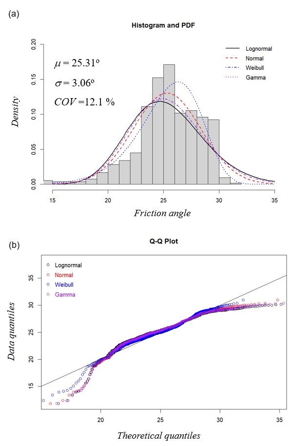
In the global analysis, a similar pattern was observed, with COV values ranging from 0.17 (17%) for the friction angle to 1.35 (135%) for the friction sleeve (f_s). The global approach also enabled evaluation of the fit of the parameters to appropriate probability density functions (PDFs) (Table 3, Figures 3 and 4). The analysis, performed in RStudio (R Core Team, 2023), tested normal, lognormal, gamma, and weibull distributions, given their established application in geotechnical engineering. Several R packages were used, in this analysis including ggplot2 and fitdistrplus. The results indicated that the lognormal distribution provided the best fit for q_c and f_s, whereas the normal distribution was more suitable for u₂ and ϕ.

Figure 3
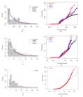
Variability analysis – coarse material: (a) q_c histogram; (b) q_c Q-Q plots; (c) f_s histogram; (d) f_s Q-Q plots; (e) u₂ histogram; and (f) u₂ Q-Q plots.

Figure 4
Variability analysis – coarse material – friction angle: (a) histogram and theoretical PDFs; (b) Q–Q plot.

Previous studies by Dienstmann et al. (2025a, b) characterized the variability of gold tailings using individual CPTu profiles to identify behavioral patterns, COV ranges, and recurring PDFs for q_c, f_s, and u₂. They reported high variability, with COV values ranging from 0.18-5.27 (18-527%), and difficulties in establishing the best-fit PDFs. The present study revealed a reduction in variability after proper profile treatment, confirming the effectiveness of this approach. In both the previous and current studies, the lognormal distribution was generally most suitable for q_c and f_s, whereas the normal distribution better represented u₂. Grouping data by characteristic behavior also improved the accuracy of distribution fitting.

5.1.2 Fine material (clay behavior)

The variability analysis for fine-grained material behavior (clay behavior) was conducted considering the results in the profile where Ic_RW >2.95. Overall, the evaluated parameters exhibited COVs ranging from 0.10 (10%) to 0.88 (88%), which, although high, suggest lower variability for the finer-grained tailings than for the coarser-grained material. In terms of spatial variation, the assessed fine-behavior layers ranged in thickness from 0.24 to 1.70 m, resulting in SOF values between 0.01 and 1.35 m (Table 4).

Table 4
Local and global variability analysis – fine material.

Data	μ		σ		COV		Layer Lenght (m)	SOF (m)	PDF
	local	global	local	global	local	global
qc (kPa)	22.30 - 354.22	251.36	10.03 - 69.97	105.7	0.11 - 0.45	0.421	0.24 - 1.70	0.05 - 0.39	N
fs (kPa)	1.10 - 5.40	3.60	0.15 - 4.46	3.1	0.12 - 0.70	0.844	0.24 - 1.70	0.01 - 0.66	LN
u2 (kPa)	8.12 - 241.02	134.50	6.75 - 29.96	69.3	0.10 - 0.88	0.515	0.24 - 1.70	0.07 - 1.35	N
Su (kPa)	3.76 - 21.69	15.06	0.77 - 5.53	7.1	0.16 - 0.63	0.471	0.24 - 1.70	0.05 - 0.90	N
Su/σ'v0	0.13 - 0.35	0.27	0.04 - 0.14	0.1	0.16 - 0.64	0.385	0.24 - 1.70	0.06 - 0.57	LN
ϕ (°)	-	25.31	-	3.1	-	0.121	-	-	W/N

• N = normal; LN = lognormal; W = weibull.

The global analysis allowed the evaluation of the probability density functions (PDFs) that best fit the measured q_c​, f_s​, and u₂​ values, as well as the derived parameters (see Table 4 and Figures 5 and 6). The parameters q_c​, u₂​, Su​, and friction angle were found to follow a normal distribution, whereas f_s​ and the normalized undrained shear strength (Su/σ_v′0) were better represented by a lognormal distribution.

Figure 5
Variability analysis – fine material: (a) q_c histogram; (b) q_c Q-Q plots; (c) f_s histogram; (d) f_s Q-Q plots; (e) u₂ histogram; and (f) u₂ Q-Q plots.

Figure 6
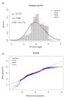
Variability analysis – fine material – friction angle: (a) histogram and theoretical PDFs; (b) Q–Q plot.

More specifically, when the undrained shear strength was analyzed, a detailed separation of the profile allowed the normal distribution to be identified as suitable for representing the parameter Su, with a mean value of 15.06 kPa and a standard deviation of 7.09 kPa (COV = 47.08%). In the approach presented by Dienstmann et al. (2025b), the lognormal distribution was proven more appropriate, with a mean value of 12.94 kPa and a standard deviation of 9.74 kPa (COV = 71.9%).

For modeling the normalized undrained strength, lognormal distributions showed good adherence, with a mean value of 0.27 and a COV of 38.52%, values close to those characterized by Dienstmann et al. (2025b). Recently, Becker et al. (2024) presented statistical data regarding the characterization of the variability in the undrained shear strength of iron tailings from the Germano site (Mariana, Minas Gerais state, Brazil). The authors performed a careful analysis to separate the data from several profiles and analyzed the distribution of the normalized undrained shear strengths. Only the layers considered to exhibit plastic behavior were analyzed, and the influence of layer thickness was also examined.

The results revealed that the distribution of the Su/σ′_v0 ratio of the plastic tailings from the Germano dam is lognormal and that the thicker a layer of plastic tailings is, the lower its normalized resistance Su/σ′_v0 and its variability. The variation range of the Su/σ′_v0 ratio obtained by the authors was 0.11-0.24, with COVs ranging from 29-47%, values generally consistent with those obtained in the present study, which revealed a mean Su/σ′_v0 ratio of 0.27 and a COV of 36.8% (Figure 7).

Figure 7
Variability analysis – fine material – undrained shear strength: (a) Su histogram and theoretical PDFs; (b) Su Q–Q plot; (c) Su/σ'_v0 histogram and theoretical PDFs; and (d) Su/σ'_v0 Q–Q plot.

5.2 Numerical application

Figures 8 and 9 provide both 3D and 2D visualizations of the Monte Carlo (MC) analyses, illustrating the variation in ​ q_c/q_cUD for the five evaluated penetration rates, considering Analyses 1 to 4 (Table 2). The results show an increase in dispersion as the normalized velocity decreases (indicating greater drainage), with maximum amplitudes of q_c/q_cUD ​ ranging from approximately 1.5 to 4 for normalized velocities of V=0.00001. The largest variation was observed in Analysis 3, which considered variability in the compressibility index (λ) modeled with a lognormal distribution and a COV of 42%. Nevertheless, the general distribution patterns remained similar among all analyses. In this context, Figure 9 was produced by combining the data from all four analyses, capturing the high variability of the site and providing a robust representation of the potential spectrum of ​q_c/q_cUD values for the material.

Figure 8
Numerical results histograms 3D (V_h versus q_c/q_cUD and density) and 2D visualization (q_c/q_cUD and density): (a) analysis 1 – 3D; (b) analysis 3 – 2D; (c) analysis 4 – 3D; (d) analysis 4 – 2D.

Figure 9
(a) Histograms 3D (V_h versus q_c/q_cUD and density); (b) 2D visualization of q_c/q_cUD and density – coarse and fine material.

The numerical analysis results were subsequently used to create a direct comparison with the range of field values, as shown in Figure 10. The normalization adopted in Figure 10 was (q_c-q_cmin)/(q_cmax-q_cmin), where q_cmin=q_cUD (undrained) and q_cmax=q_cD (drained). This normalization was effective in emphasizing the transitional shape of the drainage curves (Mafra & Dienstmann, 2022). Only the maximum and minimum curves from each numerical analysis were plotted.

Figure 10
Characteristic drainage curves considering soil variability.

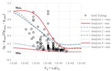
Importantly, some assumptions were made when selecting the input parameters for the numerical models, including the following:

• adoption of Equations 5 and 6 to derive the frictional parameter;

• adoption of the characterized COV and distribution of q_c​ for modeling the variability of λ;

• use of the Cam‒Clay constitutive model;

• selection of a single domain range of R (a₀=25R) in the numerical model.

Despite these considerations, good agreement was observed between the theoretical limits and the field data ranges, indicating that the variability characterization approach is a robust tool for representing behavioral limits.

6. Discussion and concluding remarks

This study details the characterization of the inherent variability of a silty deposit (gold tailings) through the analysis of piezocone tests. The data considered are part of a comprehensive campaign aimed at characterizing the geomechanical behavior of the deposit and were processed and analyzed via a layer separation algorithm and calculation of relevant statistical parameters.

Classification of profiles into drained, partially drained, and undrained behaviors proved essential for accurately characterizing the spatial variability in the strength parameters of the tailings studied. This approach enhances the understanding of the probability distributions governing CPTu data—as cone resistance (q_c), sleeve friction (f_s), and pore pressure (u₂). The results indicated that the variability associated with the q_c, f_s and u₂ measurements is greater for coarse granular materials than for finer-grained materials. However, when the strength parameters were evaluated, the fine-grained materials presented greater variability, with the highest coefficient of variation (COV) observed for the undrained shear strength (Su) compared with the friction angle (ϕ).The material behavior classification was also critical for the rigorous determination of the scale of fluctuation, which, although not applied in the numerical modeling presented herein, remains an important part of the spatial variability characterization.

The numerical application illustrates the influence of inherent variability on the expected range of normalized cone resistance (q_c/q_cUD) under different drainage conditions. The analyses revealed that greater dispersion occurred at lower normalized velocities (indicating increased drainage), with amplitudes reaching up to four times q_c/q_cUD in specific scenarios. Among the simulations, the most pronounced variability was observed when the compressibility index (λ) was modeled with a lognormal distribution and a COV of 42%. Despite the simplifying assumptions adopted for the input parameters and numerical domain, the theoretical boundaries established through the variability characterization aligned well with the field data ranges. This agreement highlights the robustness of the proposed methodology in defining realistic behavioral limits, which can support practical applications such as correcting sounding profiles or incorporating variability bounds into reliability-based geotechnical analyses.

List of symbols and abbreviations

a Radius of influence for the cavity expansion solution

a₀ Radius of the initial pore pressure zone of influence

c_h Horizontal coefficient of consolidation

d Probe diameter size

f_s Friction Sleeve

j Index for lag steps

k Permeability

l_r Element length

l_z Element height

n Number of available measurements

p₀ Total initial mean stress

p’₀ Effective initial mean stress

p’ Effective mean stress

p_c0 Reference initial consolidation pressure

q_c Cone tip resistance

q_cmin Minimum Cone tip resistance

q_cmax Maximum Cone tip resistance

q_cD Drained Cone tip resistance

q_cUD Undrained Cone tip resistance

q_t Total Cone tip resistance

r Radial distance

t(x) Deterministic trend

u Excess pore pressure

u₀ Hydrostatic pore pressure

u_0,max Maximum initial excess pore pressure

u₂ Penetration pore pressure (position 2)

w Water content

w(x) Fluctuation or residual component_.

v Loading rate

Bq Pore pressure ratio

CNPq National Council for Scientific and Technological Development

CPT Cone test

CPTu Piezocone test

COV Coefficient of variation

C(τ_j) ​ Covariance at lag distance

C(τ₁) ​ Covariance at zero lag distance

FAPESC Santa Catarina Research Foundation

Gs Specific gravity

Ic Soil Behavior Index

Ic_RW Soil Behavior Index (Robertson & Wride, 1998)

I1K Piezocone test designation (Klahold, 2013)

I1S Piezocone test designation (Sosnoski, 2016)

L Cone tip length

LN Lognormal distribution

M Friction coefficient

MC Monte Carlo

N Normal distribution

N_kt Capacity factor

NTNU Norwegian University of Science and Technology

PPGEC PostGraduate Program in Civil Engineering

PDF Probability density function

PZC Piezocone test designation

Q Normalized resistance

Q-Q plot Quantiles plot: Theoretical and Data Quantiles

R Radius

R² Coefficient of determination

SBP Soil behavior type

SCL Spatial correlation length

SCPTu Seismic piezocone test

SDMT Seismic dilatometer test

SOF Scale of fluctuation

Su Undrained shear strength

TAM Theoretical autocorrelation model adjustment

TSF Tailings storage facility

UFSC Federal University of Santa Catarina

V_h Normalized horizontal velocity

W Weibull distribution

X Considered variable

X_i Value of parameter X as depth z_i

δ Spatial correlation length/scale of fluctuation

δv Vertical spatial correlation length/vertical scale of fluctuation

Δz Minimum spacing between measurements

κ Slope of the Recompression Line (RL)

λ Slope of the Normal Consolidation Line (NCL)

μ Mean

μ_X Mean of parameter X

ν Poisson coefficient

ξ(x) Geotechnical parameter

ξ_r Radial displacement

ϕ′ Friction angle

ρ(τ_j​) Sample autocorrelation

σ Standard deviation

σ_v0 Total vertical stress at rest

σ′_v0 Vertical effective stress at rest

σ′_vt Vertical effective stress

τ_j ​ Separated lag distance between points X_i and X_i+j

Acknowledgements

This study was carried out with the support of the Santa Catarina Research Foundation (FAPESC) and the National Council for Scientific and Technological Development (CNPq). The authors also thank the Soil Mechanics Lab and the PostGraduate Program in Civil Engineering (PPGEC) of the Federal University of Santa Catarina (UFSC).

• Discussion open until August 31, 2026.
• Data availability
  The datasets generated during and/or analyzed during the current study are available from the corresponding author on reasonable request.
• Declaration of use of generative artificial intelligence
  This work was prepared with the assistance of generative artificial intelligence (GenAI) using ChatGPT (OpenAI, 2025) with the aim of supporting translation, refinement of English writing, and improvement of figure formatting. The entire process of using this tool was supervised, reviewed, and, when necessary, edited by the authors. The authors assume full responsibility for the content of the publication that involved the aid of GenAI.

References

• Abaqus. (2025). Abaqus Version 6.13. Providence, RI: Simulia Corp.
• Agbaje, S., Zhang, X., Patelli, E., Ward, D., & Dhimitri, L. (2024). Random field failure and postfailure analyses of vertical slopes in soft clays. Computers and Geotechnics, 166, 106037. https://doi.org/10.1016/j.compgeo.2023.106037
  » https://doi.org/10.1016/j.compgeo.2023.106037
• Becker, L.D.B., Aguiar, A.L.S., & Lacerda, W.A. (2024). Variability of the undrained strength of the plastic tailings from the Germano dam in Mariana, Brazil. Geomechanics and Geophysics for Geo-energy and Geo-resources, 10(1), 25. https://doi.org/10.1007/s40948-024-00750-4
  » https://doi.org/10.1007/s40948-024-00750-4
• Bedin, J. (2010). Study of the geomechanical behavior of tailings [Doctoral thesis]. Federal University of Rio Grande do Sul (in Portuguese).
• Campos, J.P., Meier, A.L., Felisbino, A., & Dienstmann, G. (2025). Inherit variability characterization considering piezocone test data: application to bauxite tailings. Mathematics and Systems Science, 3(2), 3120. https://doi.org/10.54517/mss3120
  » https://doi.org/10.54517/mss3120
• Dienstmann, G., Maghous, S., & Schnaid, F. (2017). Theoretical analysis and finite element simulation for nonlinear poroelastic behavior of cylinder expansion in infinite media under transient pore-fluid flow conditions. International Journal of Geomechanics, 17(7), 04017001. https://doi.org/10.1061/(ASCE)GM.1943-5622.0000834
  » https://doi.org/10.1061/(ASCE)GM.1943-5622.0000834
• Dienstmann, G., Schnaid, F., Maghous, S., & DeJong, J. (2018a). Piezocone penetration rate effects in transient gold tailings. Journal of Geotechnical and Geoenvironmental Engineering, 144(2), 04017116. https://doi.org/10.1061/(ASCE)GT.1943-5606.0001822
  » https://doi.org/10.1061/(ASCE)GT.1943-5606.0001822
• Dienstmann, G., Maghous, S., & Schnaid, F. (2018b). Assessment of rate effects in piezocone tests from poroelastic cavity expansion analysis. Soils and Rocks, 41(3), 319-332. https://doi.org/10.28927/SR.413319
  » https://doi.org/10.28927/SR.413319
• Dienstmann, G., Perini, L., Meier, A.L., Ziesmann, N., & Pasa, J.C. (2025a). Incorporating inherited variability into drainage effect analysis of piezocone tests in gold tailings. Proceedings of the Institution of Civil Engineers - Geotechnical Engineering, 178(2), 208-222. https://doi.org/10.1680/jgeen.23.00082
  » https://doi.org/10.1680/jgeen.23.00082
• Dienstmann, G. Perini, L. Meier, A.L. Ziesmann, N. & Pasa, J.C. (2025b). Variability characterization of a gold tailings deposit considering piezocone soundings interpretation. REM - International Engineering Journal In press.
• Fenton, G.A., & Griffiths, D.V. (2008). Risk assessment in geotechnical engineering Hoboken: John Wiley & Sons. https://doi.org/10.1002/9780470284704
  » https://doi.org/10.1002/9780470284704
• Hu, Y., & Wang, Y. (2024). Evaluating statistical homogeneity of cone penetration test (CPT) data profile using autocorrelation function. Computers and Geotechnics, 165, 105852. https://doi.org/10.1016/j.compgeo.2023.105852
  » https://doi.org/10.1016/j.compgeo.2023.105852
• Huber, M. (2013). Soil variability and its consequences in geotechnical engineering [Doctoral thesis]. University of Stuttgart.
• Kenarsari, A.E., Chenari, R.J., & Eslami, A. (2013). Characterization of the correlation structure of residual CPT profiles in sand deposits. International Journal of Civil Engineering, 11, 29-37.
• Klahold, P.A. (2013). Interpretation of field tests on soils with intermediate permeability [Master’s dissertation]. Federal University of Rio Grande do Sul (in Portuguese).
• Kulhawy, F.H., & Mayne, P.W. (1990) Manual on estimating soil properties for foundation design (Report EPRI, No. EL6800, 306 p.). Palo Alto: Electric Power Research Institute.
• Mafra, V., & Dienstmann, G. (2022). Cavity expansion solutions applied to help assess the partial drainage behavior characterization of the piezocone test. Computers and Geotechnics, 152, 105017. https://doi.org/10.1016/j.compgeo.2022.105017
  » https://doi.org/10.1016/j.compgeo.2022.105017
• Mayne, P.W., & Campanella, R.G. (2005). Versatile site characterization by seismic piezocone. In Proceedings 16th International Conference on Soil Mechanics and Geotechnical Engineering (Vol. 2, pp. 721-724), Osaka.
• Nie, X., Zhang, T., Huang, H., Liu, Z., & Lacasse, S. (2015). Scale of fluctuation for geotechnical probabilistic analysis scale of fluctuation for geotechnical probabilistic analysis. In Proceedings of the 5th International Symposium on Geotechnical Safety and Risk (Vol. 1, pp. 834-840), Rotterdam.
• Overgård, I.E. (2015). Reliability-based design of a monopile foundation for offshore wind turbines based on CPT data [Master’s dissertation]. Norwegian University of Science and Technology.
• Phoon, K.-K., & Kulhawy, F.H. (1999). Characterization of geotechnical variability. Canadian Geotechnical Journal, 36(4), 612-624. https://doi.org/10.1139/t99-038
  » https://doi.org/10.1139/t99-038
• Phoon, K.-K., Cao, Z.-J., Ji, J., Leung, Y.F., Najjar, S., Shuku, T., Tang, C., Yin, Z.-Y., Ikumasa, Y., & Ching, J. (2022). Geotechnical uncertainty, modeling, and decision making. Soil and Foundation, 62(5), 101189. https://doi.org/10.1016/j.sandf.2022.101189
  » https://doi.org/10.1016/j.sandf.2022.101189
• Pieczyńska-Kozłowska, J., Bagińska, I., & Kawa, M. (2021). The identification of the uncertainty in soil strength parameters based on cptu measurements and random fields. Sensors, 21(16), 5393. https://doi.org/10.3390/s21165393
  » https://doi.org/10.3390/s21165393
• R Core Team. (2023). R: a language and environment for statistical computing. Vienna: R Foundation for Statistical Computing.
• Robertson, P.K., & Wride, C.E. (1998). Evaluating cyclic liquefaction potential using the cone penetration test. Canadian Geotechnical Journal, 35(3), 442-459. https://doi.org/10.1139/t98-017
  » https://doi.org/10.1139/t98-017
• Salgado, R., Prezzi, M., & Ganju, E. (2015). Assessment of site variability from analysis of cone penetration test data (No. FHWA/IN/JTRP-2015/04, 132 p.). West Lafayette: Joint Transportation Research Program, Indiana Department of Transportation and Purdue University. https://doi.org/10.5703/1288284315523
  » https://doi.org/10.5703/1288284315523
• Schnaid, F., Odebrecht, E., Sosnoski, J., & Robertson, P.K. (2016). Effects of test procedure on flat dilatometer test (DMT) results in intermediate soils. Canadian Geotechnical Journal, 53(8), 1270-1280. https://doi.org/10.1139/cgj-2015-0463
  » https://doi.org/10.1139/cgj-2015-0463
• Schnaid, F., Dienstmann, G., Odebrecht, E., & Maghous, S. (2020). A simplified approach to normalisation of piezocone penetration rate effects. Geotechnique, 70(7), 630-635. https://doi.org/10.1680/jgeot.18.T.033
  » https://doi.org/10.1680/jgeot.18.T.033
• Senneset, K.R., Sandven, T., & Janbu, N. (1989). Evaluation of soil parameters from piezocone tests (Transportation Research Record, no. 1235, pp. 24-37). Washington: Transportation Research Board, National Research Council.
• Senneset, K., Sandven, R., Lunne, T., By, T., & Amundsen, T. (1988). Piezocone tests in silty soils. In Penetration Testing 1988: Proceedings of the First International Symposium on Penetration Testing (Vol. 2, pp. 955-974). Rotterdam: Balkema.
• Sosnoski, J. (2016). Interpretation of CPTU and DMT tests in intermediate permeability soils [Master’s dissertation]. Federal University of Rio Grande do Sul (in Portuguese).
• Uzielli, M., Lacasse, S., Nadim, F., & Phoon, K.K. (2007). Soil variability analysis for geotechnical practice. In T. S. Tan, K. K. Phoon, D. W. Hight & S. Leroueil (Eds.), Characterization and engineering properties of natural soils (Vol. 3-4, pp. 1653-1752). London: Taylor & Francis.
• Vanmarcke, E.H. (1977). Probabilistic modeling of soil profiles. Journal of Geotechnical Engineering, 103, 1227-1246.

Edited by

• Editor:
  Renato P. Cunha https://orcid.org/0000-0002-2264-9711

Data availability

The datasets generated during and/or analyzed during the current study are available from the corresponding author on reasonable request.

Publication Dates

• Publication in this collection
  26 Jan 2026
• Date of issue
  2026

History

• Received
  16 Aug 2025
• Accepted
  03 Nov 2025