From satellites to yield: causal modeling of paddy rice production using sparse regression and dynamic remote sensing

ABSTRACT:

This study presents a novel approach that combines agricultural census data with remotely sensed time series to develop accurate predictive models for paddy rice yield across the different regions of Peru. By leveraging sparse regression and Elastic-Net regularization techniques, the study uncovers causal relationships between key remotely sensed variables such as Normalized Difference Vegetation Index (NDVI), precipitation (PREC), temperature (TEMP), and agricultural yield. To further enhance prediction accuracy, first- and second-order dynamic transformations (velocity and acceleration) of these variables were applied to capture non-linear patterns and lagged effects on yield. The findings demonstrate improved predictive performance when integrating regularization techniques with climatic and geospatial variables, allowing for more accurate forecasts of yield variability. The results confirm the presence of causal relationships in the Granger sense, underscoring the value of this methodology to strategic agricultural management. This contributes to more efficient and sustainable production in paddy rice cultivation.

Keywords:
Elastic-Net regularization; Granger Causality; NDVI; satellite data; sparse regression

Introduction

Precision agriculture is advancing rapidly with the integration of technologies such as pattern recognition, machine learning, and remotely sensed data (Liakos et al., 2018; Kussul et al., 2017). These innovations have significantly enhanced the accuracy of crop yield forecasting by analyzing large datasets and uncovering hidden patterns, enabling better predictions, problem detection, and resource optimization, with recent research demonstrating that integrating multi-source satellite data with machine learning and deep learning models significantly improves rice yield estimation accuracy (Cao et al., 2021). However, in Peru, the use of machine learning algorithms for satellite image classification has primarily focused on land cover analysis and environmental monitoring, with limited applications specifically targeting yield forecasting (Baquerizo and Ventocilla, 2022).

This study focused on how machine learning, combined with climatological and geospatial data, can improve the prediction of agricultural yields. Specifically, we aimed to investigate the causal relationships between remote sensing variables (such as Normalized Difference Vegetation Index (NDVI), precipitation, and temperature) and crop yields. Additionally, recent findings suggest that the integration of remote sensing and deep learning, particularly when supported by cloud computing platforms, provides a viable and scalable approach for improving paddy yield estimation (Asmar et al., 2024). Therefore, we also sought to use these relationships to build simple machine learning models for forecasting, using rice yield data from Peru as a case study.

Research on rice yield forecasting in Peru is limited, especially in the field of the use of advanced techniques, and this study aimed to fill that gap by applying machine learning methods such as sparsity, regularization, and remote sensing data to enhance forecasting accuracy.

Key methodologies include the integration of remote sensing data with the National Agricultural Survey (NAS) and the use of Elastic-Net regression, which balances variable selection and parameter regularization. This approach helped identify causal relationships between remote sensing data and yields (Wood, 2017). We also applied sparsity-inducing techniques and Generalized Additive Models (GAM) to capture nonlinear relationships, as well as the XGBoost model for more flexible and accurate yield predictions. The results from these models were compared with those obtained using the Elastic-Net approach.

Materials and Methods

Area of study

As mentioned earlier, we used paddy rice production in Peru as a case study for our methodologies. This cereal has a growth cycle with clearly defined stages, which is essential to an understanding of its yield and productivity in different study areas. In this context, the growth cycle of this cereal begins with germination, during which the seeds absorb water, and the radicle emerges. Next, in the seedling phase, the first true leaves appear. During the vegetative phase, the plant experiences rapid foliar growth and accumulates essential nutrients. Similarly, the panicle initiation phase marks the beginning of reproductive development, culminating in flowering and pollination. Finally, during the grain filling phase, the grain forms and matures, concluding the cycle and leading to harvest. It is important to note that the duration and characteristics of each stage may vary depending on environmental conditions and management practices implemented in each region. Therefore, several regions in Peru were selected as study areas, focusing on those with the highest concentrations of paddy rice production. The primary source of information for this analysis comes from agricultural censuses conducted in Peru between 2015 and 2018, which provide detailed and updated data on agricultural practices and characteristics. These data were obtained from the Plataforma Nacional de Datos Abiertos, and further details on data access can be found in the Data Availability section.

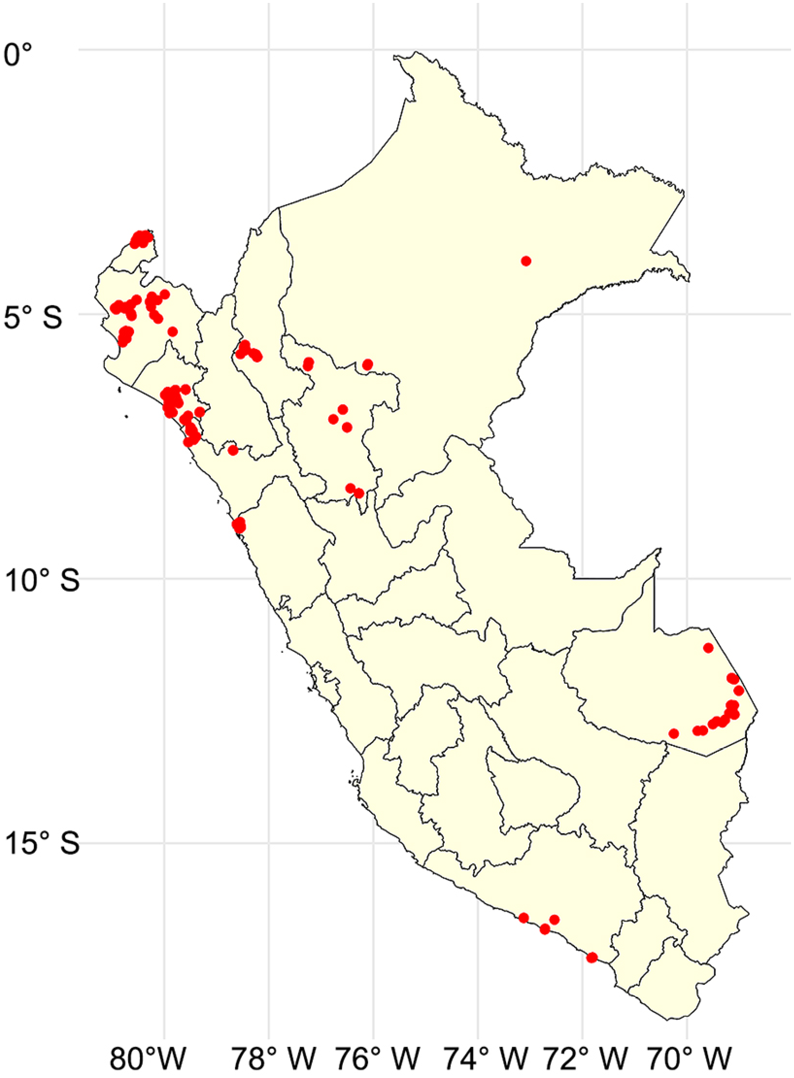
For model training, 80% of the data was used. To ensure the proper organization and georeferencing of the collected data, a specific coding system was developed. This system allows for the identification of the location of each study area, facilitating both spatial and temporal analysis. The coding includes the department code (CCDD), which identifies the administrative region; the province code (CCPP), which specifies the subdivision within the department; the district code (CCDI), which details the local subdivision; and the cluster code, which groups smaller areas or sampling units within a district. The location refers to the central point of the plot, and each location has a single sample. Additionally, latitude and longitude coordinates were incorporated, as shown in Table 1, which illustrates the implementation of this coding system in the project. This highlights its applicability in identifying and monitoring paddy rice production areas over time. Furthermore, a map showing the distribution of farms within the study area is available in Figure 1.

Table 1
The table below presents the location variables as follows: coding includes the department code (CCDD) representing the administrative region; province code (CCPP) specifying the subdivision within the department; district code (CCDI) detailing the local subdivision within a province; and CONGL groups the sampling areas within a district. Latitude (LAT) and longitude (LONG) indicate the precise geographic coordinates of the paddy rice fields.

Geographic and administrative data of sampling locations
ID	Year	CCDD	CCPP	CCDI	CONGL	LAT	LONG
1	2018	1	2	3	5198	–5.676	–78.438
2	2018	1	7	2	5318	–5.806	–78.219
3	2018	1	7	2	5318	–5.808	–78.219
4	2017	2	18	1	8260	–9.006	–78.540
5	2016	2	18	1	8250	–8.955	–78.580
6	2017	20	1	9	1132	–5.372	–80.707

Figure 1
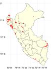
Georeferenced locations of rice crops used for information extraction, represented on the map of Peru. Each point indicates the exact location of the analyzed samples, allowing for the visualization of the spatial distribution of the crops across the territory.

The field experiments were conducted at a representative location with geographic coordinates 8°55’57" S, 78°34’51" W, altitude 44 m. The coordinates for all evaluated points were sourced from a satellite database. The complete set of locations can be accessed through this link: https://goo.su/6W6MA

Remote sensing data

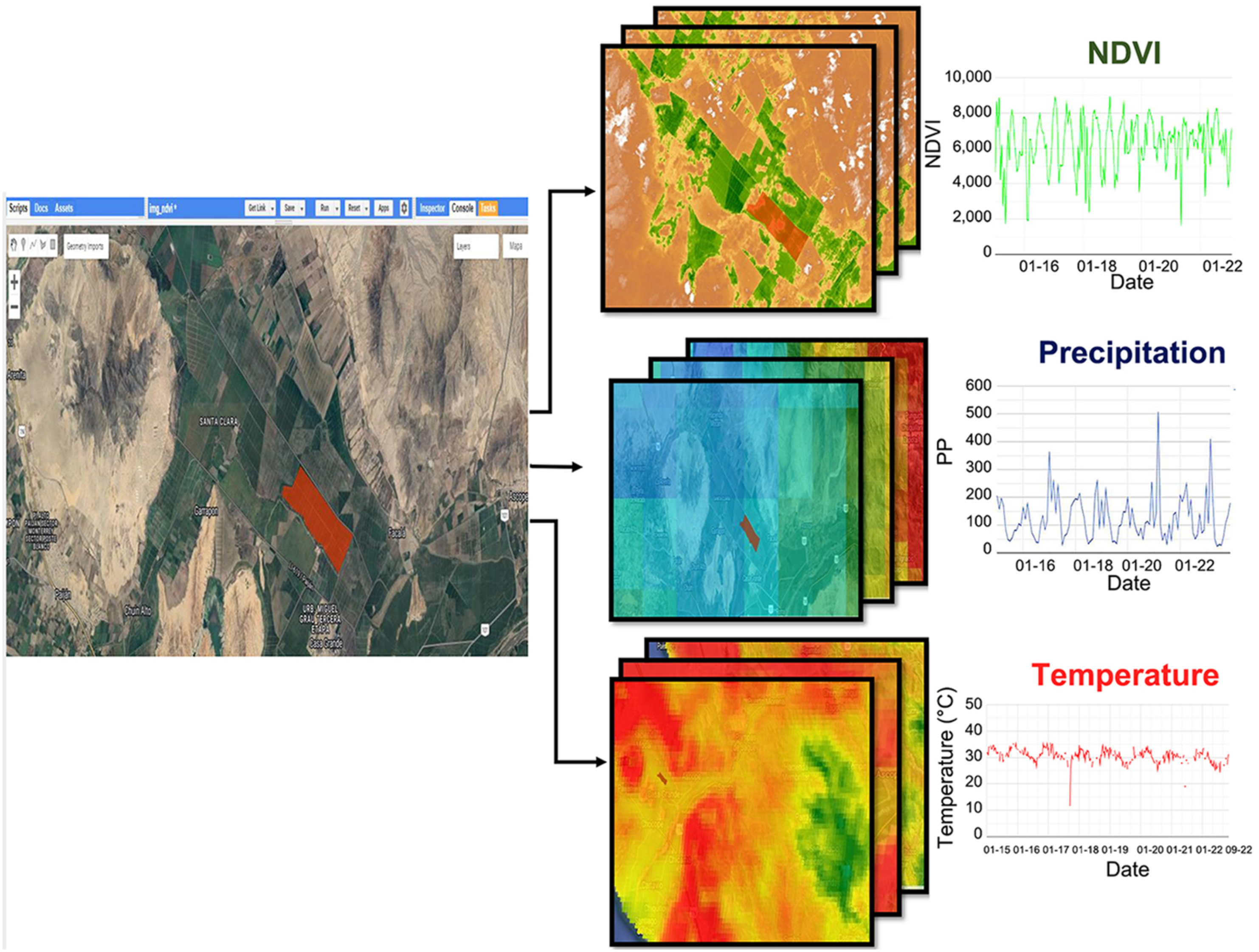
The satellite images used in this study were obtained through remote sensing and processed using open-access tools such as Google Earth Engine (GEE). In this platform, radiometric and atmospheric corrections are applied, along with the management of cloud-induced variability, to ensure high-resolution images (Saunders and Kriebel, 1988). Although GEE provides pre-corrected data, the additional corrections made ensure that the data used in this study are accurate, consistent, and specific to the local conditions and the rice crops in the analyzed plots. Therefore, these images are essential to generating precise information based on relevant indices, as illustrated in Figure 2. Key remote sensing variables that significantly influence crop development and yield were identified and selected. The first of these is the NDVI, a crucial metric for assessing vegetation health. It is calculated according to Eq. (1):

Figure 2
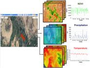
The graphic illustrates the process of extracting remotely sensed time series using Google Earth Engine. On the right, three images are shown, each color-coded to represent a different type of series: normalized difference vegetation index (NDVI), precipitation (PREC), and temperature (TEMP).

(1) $$NDVI=\frac{\text{ρ}NIR-\text{ρ}RED}{\text{ρ}NIR+\text{ρ}RED}$$

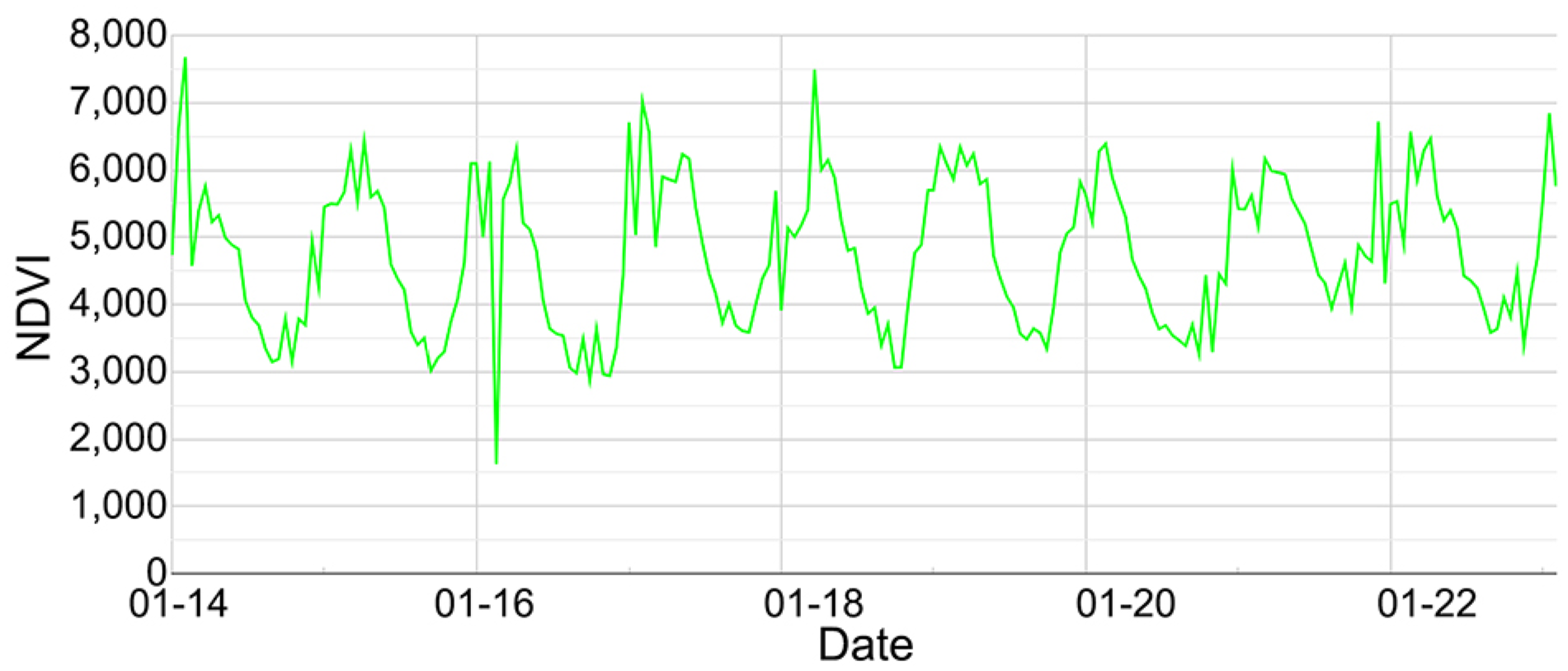
where NIR is the near infrared reflectance band and RED is the red band. The data for this variable were obtained through the MOD13Q1 sensor, which generates NDVI time series with a frequency of 16 days (Volante et al., 2015). This sensor allows for categorizing land surface properties and biological processes, as well as primary production and land cover changes. The NDVI series sampled is shown in Figure 3.

Figure 3
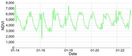
The graph presents a time series of the normalized difference vegetation index (NDVI) with a 16-day frequency, obtained using the MOD13Q1 product from the MODIS satellite, with a spatial resolution of 250 m.

The second variable is PREC, which directly affects soil moisture and is therefore a critical factor in crop growth (Liu et al., 2015). Although the specific formula for determining PREC using the CHIRPS Pentad dataset is not explicitly provided, the process involves combining satellite-derived infrared precipitation estimates with in situ weather station data (Funk et al., 2014). In this study, we used CHIRPS Pentad Version 2.0, which provides quasi-global rainfall data at 0.05° spatial resolution from 1981 to the present. The general procedure can be described as follows:

(2) $$PREC=f(S,T,C),$$

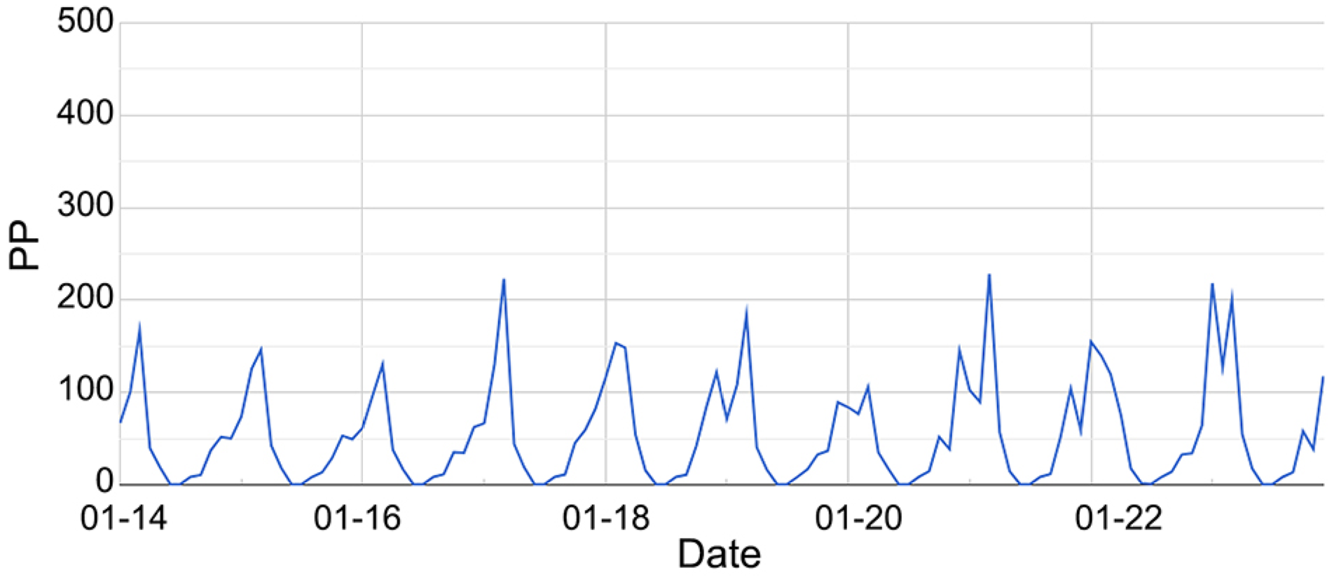
where PREC represents the estimated precipitation, S corresponds to satellite data, T refers to ground station data, and C includes applied corrections and adjustments. This process generates PREC time series in a gridded format, which is helpful for trend analysis and seasonal drought monitoring. The sampled PREC time series is shown in Figure 4.

Figure 4
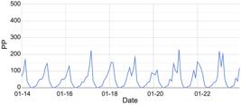
Time series of monthly precipitation (PP, in millimeters) from 2014 to 2023, based on the CHIRPS dataset. PP stands for "precipitation." The data reflect rainfall patterns relevant to the study area.

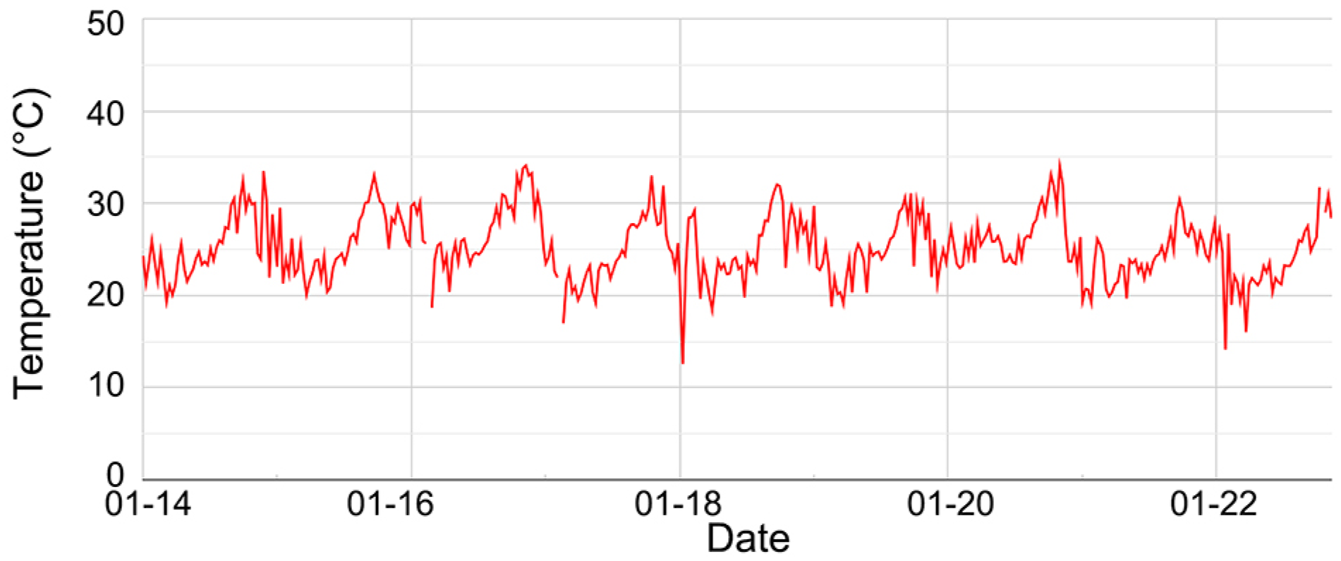
Finally, the third remote sensing variable is TEMP, which plays a crucial role in crop germination and development (Chung et al., 2012). This variable was obtained using the MOD11A1 sensor. Although no specific expression is provided by the dataset, the general formulation used to estimate land surface temperature (LST) is presented in Eq. (3):

(3) $$TEMP=\alpha +b\left(T_{31}+T_{32}\right)+c\left(T_{31}-T_{32}\right)+d{\left(T_{31}-T_{32}\right)}^2,$$

where LST represents the land surface temperature, and T₃₁ and T₃₂ are the brightness temperatures in bands 31 and 32, respectively (Guha et al., 2019). The coefficients a, b, c, d are empirically determined and vary with atmospheric and surface conditions. To estimate land surface TEMP, algorithms that combine satellite data with weather station observations are employed. The sampled TEMP time series is shown in Figure 5.

Figure 5
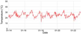
The graph presents a time series of land surface temperature (LST), measured daily in degrees Celsius using the MODIS MOD11A1 sensor, covering the period from June 2014 to Sept 2023. Although discontinuities in LST values are observed, these could be attributed to factors such as cloud cover, changes in land cover, or failures in data capture.

Data preprocessing

Precision agriculture is rapidly advancing with the integration of technologies such as pattern recognition, machine learning, and remotely sensed data. This study demonstrates that remote sensing variables contain valuable predictive information about agricultural production. To ensure the integrity of the analysis, it is essential to homogenize both the temporal frequency and the quality of the data obtained from remote sensing (NDVI, PREC, TEMP) and the agricultural census. Since the raw series had different frequencies, such as NDVI with observations every 16 days (Figure 3), PREC with monthly records (Figure 4), and TEMP with daily data (Figure 5), Spline interpolation was applied (Martínez & Gilabert, 2009; Wongsai et al., 2017). This method is suitable for handling time series with temporal irregularities, as it preserves smoothness and internal variability. Therefore, as for NDVI, weekly values were interpolated between existing observations, adjusting a Spline curve to the seasonal trend of NDVI. For PREC, the monthly series were redistributed into weeks using a weighting based on historical climate patterns, refined with Spline to smooth transitions. Finally, the daily TEMP data were aggregated to a weekly frequency by calculating the moving average, followed by Spline interpolation to correct discontinuities or outliers. Consequently, the three series (NDVI, PREC, and TEMP) were standardized to a weekly frequency using the aforementioned interpolation methodologies.

Additionally, considering the complex and highly nonlinear nature of the relationships between the remote sensing variables and agricultural yield, we chose to include both first- and second-order variations of the NDVI, PREC, and TEMP variables, along with their respective time lags. Due to the physical interpretation of these first- and second-order differences, we refer to these new variables as the velocities and accelerations of the remotely sensed variables. For instance, NDVI velocity (also defined analogously for the Precipitation and Temperature variables) is described as the rate of change in NDVI values between consecutive periods:

(4) $$VE{L}_{NDVIt}:=△NDV{I}_t=NDV{I}_t-NDV{I}_{t-1}$$

where NDVIt is the NDVI corresponding to week t. Additionally, NDVI acceleration, analogously defined for the Precipitation and Temperature variables, represents the change in NDVI velocity between consecutive periods:

(5) $$ACCE{L}_{NDVIt}:={\text{Δ}}^{2}NDV{I}_t=VE{L}_{NDVIt}-VEL\text{\_}NDV{I}_{t-1}$$

Once the velocity and acceleration variables were defined for the three series, we also incorporated the lags of up to 12 weeks for these new variables into the analysis. Specifically, the following sequences of variables were considered:

(6) $${\left\{VE{L}_{-}ND{V}_{t-d}\right\}}_{d=1}^{12},{\left\{ACCE{L}_{-}NDV{I}_{t-d}\right\}}_{d=1}^{12},$$

(7) $${\left\{VE{L}_{-}PRE{C}_{t-d}\right\}}_{d=1}^{12},{\left\{ACCE{L}_{-}PRE{C}_{t-d}\right\}}_{d=1}^{12},$$

(8) $${\left\{VEL\text{\_}TEM{P}_{t-d}\right\}}_{d=1}^{12},{\left\{ACCEL\text{\_}TEM{P}_{t-d}\right\}}_{d=1}^{12}.$$

These newly derived variables allow us to capture higher-order dynamic relationships that would be difficult to detect using the original variables alone. An important finding in this study, as we will demonstrate, is that these new variables significantly improve the predictive capacity of the models. They enable us to incorporate dynamic effects into the relationships in a straightforward manner.

Data Set

The development of the dataset for this study involved several key considerations. First, we ensured that the crop under study was homogeneous, focusing on agricultural areas where only one type of crop was grown, which allowed for more accurate data collection. Additionally, we selected a transitory crop, which undergoes distinct phenological stages such as sowing, growth, and harvest. Another crucial criterion was the ability to observe and distinguish the crop using satellite imagery. For these reasons, along with its social importance, we chose to study paddy rice, a crop of significant relevance in Peru that met all the above criteria.

Once the crop areas were identified, we proceeded with the extraction of their variables and characteristics, drawing on two main data sources. The first source was the NAS, which includes variables characterizing the use of good agricultural practices on the farms associated with the sampled crop areas. The second data source consisted of remote sensing data, extracted using open-access tools such as GEE. For this source, we developed specific algorithms to obtain spatial information on NDVI, PREC, and TEMP using latitude, longitude, and multispectral images. Each crop plot has a time series of data, and we also aggregated all the information from each plot for model generation, which consisted of 348 plots selected according to the previously mentioned filter. These series were then interpolated to obtain weekly observations, with lags of up to 12 weeks before the harvest date. Therefore, it is important to highlight that the limitations related to inaccuracies in the geographic information system for rice cultivation provided by the NAS required significant resources for data cleaning and correction. This, combined with the limited resources available to the study, resulted in the identification of only 348 paddy rice plots in different regions in Peru. However, with additional resources, we could significantly expand the sample size, thereby strengthening our results and conclusions. Finally, after completing the variable engineering process, which involved creating velocity and acceleration variables from remote sensing data, we integrated this information with control variables extracted from the NAS, as shown in Table 2. This integration resulted in a complete dataset of 348 records, which served as the basis for the analysis conducted in the modeling phase described in detail below.

Table 2
Labels, descriptions and sources of the variables used.

Variables and descriptions for paddy rice analysis
Label	Description	Source
Prod_Hect	Agricultural production of paddy rice measured in tons per hectare	NAS
P204_TIPO	Type of crop. 1: Homogeneous and 2: Heterogeneous	NAS
P206_INI	Harvest start date	NAS
P208	Crop management. 1: Homogeneous, 2: Associated, and 3: Dispersed	NAS
P211_1	When planting paddy rice, did you consider the climate of the area? 0: No, 1: Yes	NAS
P211_2	When planting paddy rice, did you consider the availability of water? 0: No, 1: Yes	NAS
P211_4	When planting paddy rice, did you consider the type of soil? 0: No, 1: Yes	NAS
P212	The water for irrigating the crop comes from 1: Rain, 2: River, 3: Spring, 4: Groundwater, 5: Reservoir, 6: Dam, 7: Other	NAS
P213	The irrigation system used was 1: Exudation, 2: Drip, 3: Microsprinkler, 4: Sprinkler, 5: Multi-gates, 6: Hoses, 7: Gravity, 8: Others	NAS
P214	The seed used was… 1: Certified, 2: Non-certified	NAS
NDVIt	NDVI corresponding to the week of paddy rice harvest t	Remote Sensing
PRECt	Precipitation corresponding to the week of paddy rice harvest t	Remote Sensing
TEMPt	Temperature corresponding to the week of paddy rice harvest t	Remote Sensing
∆ NDVIt	Velocity of the NDVI corresponding to the week of harvest t	Remote Sensing
∆ PRECt	Velocity of Precipitation corresponding to the week of harvest t	Remote Sensing
∆ TEMPt	Velocity of Temperature corresponding to the week of harvest t	Remote Sensing
∆2 NDVIt	Acceleration of the NDVI corresponding to the week of harvest t	Remote Sensing
∆2 PRECt	Acceleration of Precipitation corresponding to the week of harvest t	Remote Sensing
∆2 TEMPt	Acceleration of Temperature corresponding to the week of harvest t	Remote Sensing

• NAS = national agricultural survey; NDVI = normalized difference vegetation index.

Modeling Phase

The final dataset considered for this study is composed of $D={\left\{\left(x_i,y_i\right)\right\}}_{i=1}^N,$, where N = 348 represents the number of sampled plots. Here, the response variable yi ∈ ℝ, labeled as Prod-Hect, denotes the agricultural yield of the crop, measured in tons per hectare, when the harvest occurred in week Ti. Additionally, the covariate vector xi ∈ ℝ⁸¹ consists of two groups of variables.

The first group, denoted by zi ∈ ℝ⁹, includes variables that characterize the application of good agricultural practices for crop i. This set of variables is defined as follows:

(9) $$\begin{array}{r}\hfill Z_i=(P204\_TIP{O}_{i,}P206\_IN{I}_{i,}P{208}_{i,}P{211}_{-}{1}_{i,}\\ \hfill P{211}_{-}{2}_{i,}P211\_4_{i,}P{212}_{i,}P{213}_{i,}P213\text{i}),\end{array}$$

where the labels are described in Table 2. It is important to note that the variables comprising Zi were extracted from the ENA, corresponding to the year immediately following the harvest week Ti. The second group consists of the series $VEL\_NDV{I}_{t,}^i$, $ACCEL\_NDV{I}_{t,}^i$, $VEL\_PRE{C}_t^i$, $ACCEL\_PRE{C}_t^i$, $VEL\_TEM{P}_t^i$, and $ACCEL\_TEM{P}_t^i$, where the superscript i indicates that these series pertain to crop i. This group is expressed in Eq.(10):

(10) $$\begin{array}{ll}{w}_i=\hfill & ({\left\{VEL\_NDV{T}_{T_{l-d}}^i\right\}}_{d=1}^{12},{\left\{ACCEL\_NDV{T}_{T_{l-d}}^i\right\}}_{d=1}^{12},\hfill \\ \hfill & {\left\{VEL\_PRE{C}_{T_{l-d}}^i\right\}}_{d=1}^{12},{\left\{ACCEL\_PRE{C}_{T_{l-d}}^i\right\}}_{d=1}^{12},\hfill \\ \hfill & {\left\{VEL\_TEM{P}_{T_{l-d}}^i\right\}}_{d=1}^{12},{\left\{ACCEL\_TEM{P}_{T_{l-d}}^i\right\}}_{d=1}^{12}).\hfill \end{array}$$

Therefore, the full covariate vector xi, which consists of 81 variables, is defined by combining both groups as follows in Eq. (11):

(11) $$x_i=\left(z_i,w_i\right)$$

Finally, our dataset D ∈ ℝ^{348 × 82} includes both cross-sectional and longitudinal variables that, as will be shown later, effectively characterize the corresponding agricultural yields. This dataset encompasses remote sensing variables related to climatic and geospatial conditions up to 12 weeks prior to the harvest. As will be discussed later, these temporal lags will enable us to identify causal relationships between these variables and agricultural yield. Next, having established the database for this study, we will outline the three methodologies we will employ to obtain our results and conclusions.

Regression with Elastic-Net Regularization

Given the dataset D, our objective is to forecast agricultural yield yi using the predictors xi defined earlier. To achieve this, we assume a linear regression structure between the variables:

(12) $$y_i={\text{β}}_0+x_i^T\text{β}+{\text{ξ}}_i,$$

where the intercept β₀ and the weights β = (β₁, …, β₈₁) are unknown parameters, and ξ_i represents the error term. Since our goal is to construct a simple and parsimonious model and given that we have a large number of predictor variables that are closely related, we choose to induce moderate sparsity in the parameter vector. Therefore, to obtain the parameter estimates $\left({\widehat{\text{β}}}_0,\widehat{\text{β}}\right)$, we opt for Elastic-Net regularization (Zou and Hastie, 2005), which involves solving the convex optimization problem:

(13) $$\left({\text{β}}_0,\text{β}\right)\stackrel{\min }{\in ℝ}\times {ℝ}^{81}\left\{\frac{1}{2}{\displaystyle \sum }_{i=1}^N{\left(y_i-{\text{β}}_0-x_i^T\text{β}\right)}^2+\text{λ}\left[\frac{1}{2}(1-\text{α})\Vert \text{β}{\Vert }_2^2+\text{α}\Vert \text{β}{\Vert }_1\right]\right\},$$

where represents the standard ℓ^p norm. The penalty hyperparameter λ ≥ 0 controls the complexity of the resulting model, while the hyperparameter 0 ≤ α ≤ 1 governs the desired level of sparsity. For more details, see Hastie et al., 2015. We chose to set α = 0.02, which assigns more weight to the ℓ² norm compared to the ℓ¹ norm. This asymmetry in the weights results in a calibration of the induced sparsity in the parameter vector β that aligns with qualitative field criteria regarding the expected relationships.

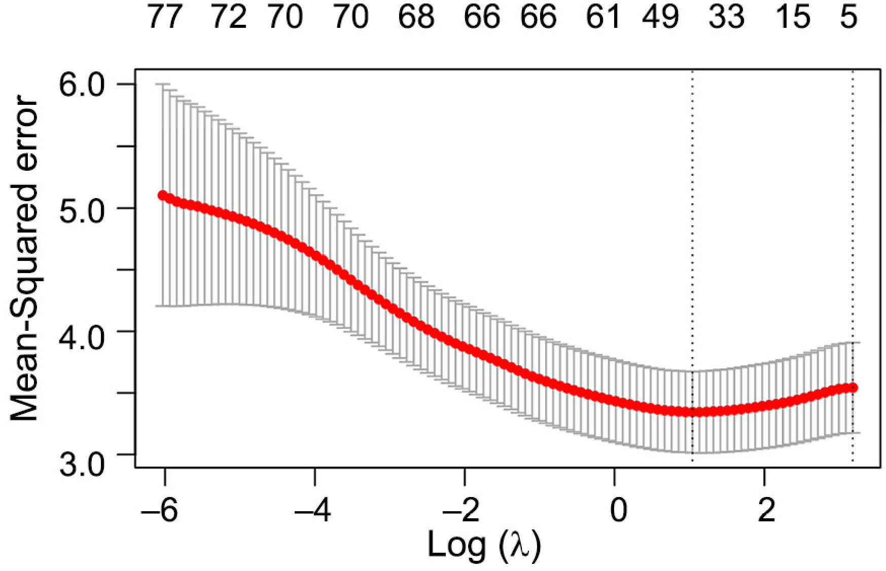
To determine the optimal value of λ, we employed the standard cross-validation criterion, evaluating the mean squared error (MSE) of the cross-validation for different values of λ on a logarithmic scale, as shown in Figure 6. This procedure yielded an optimal value of λ = 2.58. Finally, once both hyperparameters were calibrated, we solved the problem in Eq. (13) using convex optimization algorithms extensively detailed in Hastie et al. (2015). Consequently, the solution to Eq. (13) provided us with a sparse estimate of the parameter vector for the model in Eq. (12).

Figure 6
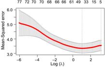
Graph to determine the optimal value of l. Vertical axis: the mean squared error (MSE) calculated through cross-validation. Horizontal axis: values of l on a logarithmic scale. The red line represents the average value of the MSE, and the gray bands represent their respective confidence intervals.

Gradient Tree Boosting

Let q: ℝ⁸¹ → T represent the structure of a tree that maps the characteristics of a crop xi to the index of the corresponding leaf. The weight vector of its leaves is given by ω = (ω₁, …, ω₁T₁ ∈ ℝ₁T₁), where ωk denotes the score of the k-th leaf. Here, T is the set of leaves of the tree, and ₁T₁ indicates the total number of leaves. To obtain the prediction of agricultural yield ${\widehat{y}}_i$1, we used an additive ensemble κ of these trees, denoted by φ, which can be expressed as follows:

(14) $${\widehat{y}}_i=\varphi \left(x_i\right)={\displaystyle \sum }_{k=1}^k{f}_k\left({\mathit{\text{x}}}_i\right),f_k\in F$$

where ℱ = {f: ℝ⁸¹→ ℝ ₁ f(xi) = ωq₍xi₎} denotes the space of regression trees, also known as CART (Breiman et al., 1984). It is important to note that each fk corresponds to an independent tree structure q with its associated leaf weights ω.

Based on the dataset D, the learning of the functions fk used in the model in Eq. (14) is achieved by solving the regularized optimization problem:

(15) $$\underset{f_k\in \mathcal{F},\forall k}{\min }{\displaystyle \sum }_{i=1}^N{\left({\widehat{y}}_i-y_i\right)}^2+{\displaystyle \sum }_{k=1}^{\kappa }\left\{\gamma \left|\mathcal{T}\right|+\frac{1}{2}\kappa \Vert \omega {\Vert }_2^2\right\}$$

where the hyperparameter γ penalizes complexity due to the depth of the trees, and λ regularizes the weights of the trees to prevent overfitting. The standard learning algorithm used to solve Eq. (15) is based on gradient methods, which is why this model is commonly referred to as Gradient Tree Boosting (XGBoost) (Chen and Guestrin, 2016). The hyperparameters in Eq. (15) are calibrated using established methodologies. Specifically, we perform optimal selection through n-fold cross-validation, as illustrated in Figure 7. Through this procedure, we obtain optimal values of γ = 0.1 and κ = 0.6. In addition to regularizing the set of tree leaves T, we optimally limited the maximum depth of the trees to 5.

Figure 7
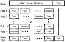
In the figure, a schematic representation of n-fold cross-validation can be observed, where in each iteration, one fold is used for validation while the remaining folds are used for training. This process is repeated n times to identify the optimal combination of hyperparameters.

Semi-parametric Additive Model

As a semi-parametric alternative, we chose a GAM structure, which can be expressed in our case as follows:

(16) $${\widehat{y}}_i={\text{θ}}_0+{\mathbf{z}}_i^T\text{θ}+{\displaystyle {\sum }_{j=1}^{72}{f}_j}\left({\mathit{\text{w}}}_i^{(j)}\right),$$

where ${\mathit{\text{w}}}_i^{(j)}$ is the j-th coordinate of the vector defined in Eq. (10). In this model, θ ∈ ℝ⁹ represents a parameter vector, θ0 ∈ ℝ is the intercept, and fj are smooth functions to be estimated using the dataset D. To estimate the model in Eq. (16), we adopted the widely used approach of representing the functions fj with reduced-rank smoothing splines that result from solving variational problems. For more details, see Zou and Hastie (2005).

Results

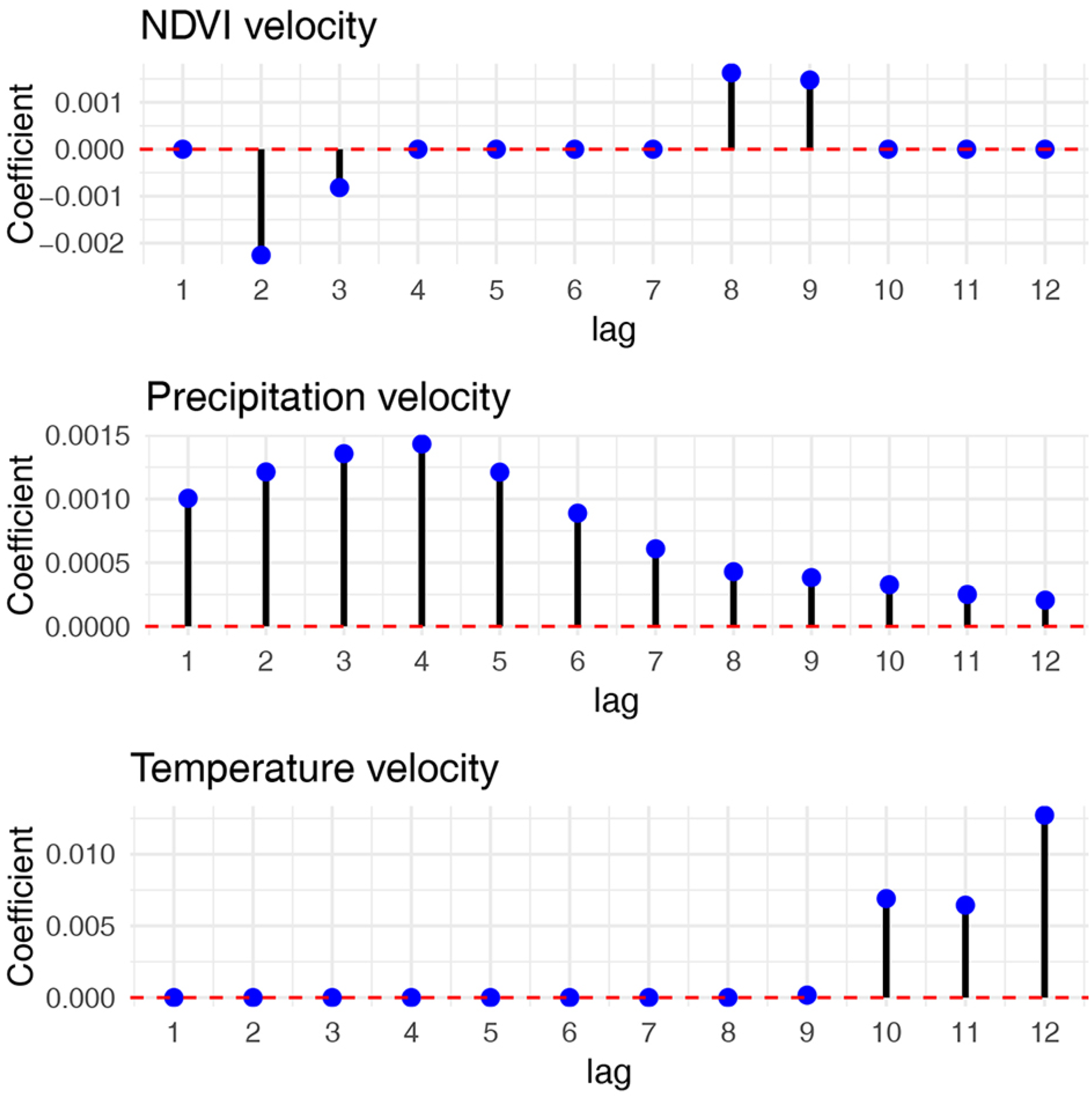
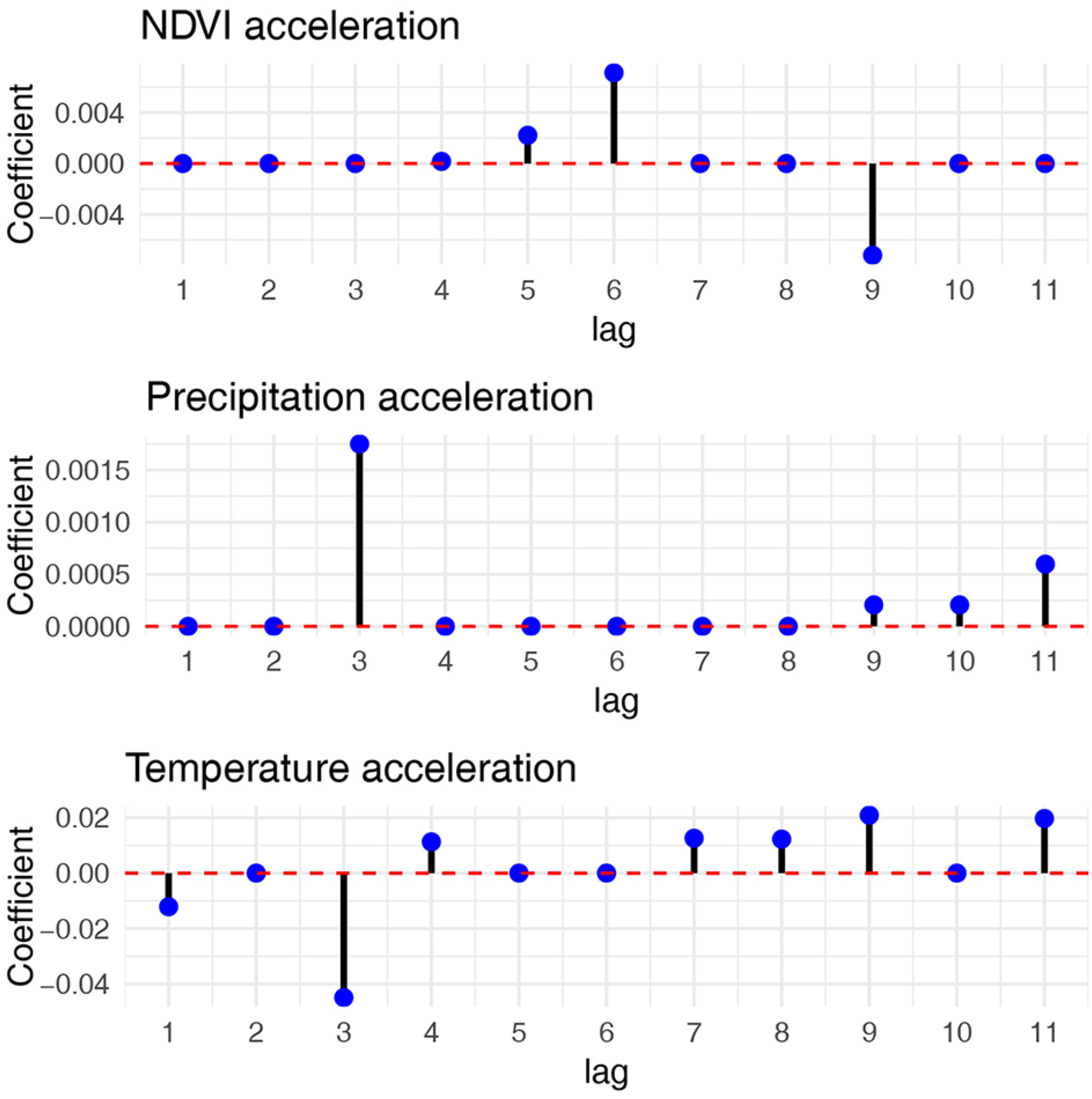
As mentioned earlier, we have two groups of predictor variables. The first group, zi, consisted of variables that characterize the use of good agricultural practices in crops. These variables serve as control variables; that is, we were not interested in their direct effects but rather the use of them to control the influences of other factors that may affect the relationship between the predictors and the response variable. The second group, wi, included the velocities and accelerations of the remote sensing variables, specifically the velocities and accelerations of NDVI, PREC, TEMP, and their respective time lags, as defined in Eq. (4), Eq. (5), and Eq. (10). Our primary interest in this study was to understand the causal relationships between the remote sensing variables and agricultural yield, particularly focusing on the parameters (or coefficients) associated with the variables in the vector wi. As regards the velocity variables, the parameter vectors obtained from model Eq. (12) through Eq. (13) for NDVI and TEMP are highly sparse, in contrast to the parameter vector for PREC, which is dense; see Figure 8. The sparsity in the velocities of NDVI and TEMP suggests that the effects of variations in these variables on agricultural yield are delayed. For instance, first-order variations in NDVI affect agricultural yield only eight or nine weeks after they occur, as shown in Figure 8. A similar pattern is observed with TEMP variations, which have a lag of 10 to 12 weeks. It is important to note that these lag periods are not precise and may vary depending on the sample. Therefore, variations in these two variables do not immediately impact agricultural yield. This delay in the influence of both climatic variables could be related to the crop germination process. In contrast, variations in PREC have an immediate and lasting effect on agricultural yield. The scenario changes when considering the acceleration variables: second-order variations in NDVI impact agricultural yield between six and nine weeks later, while similar variations in PREC and TEMP affect it approximately three weeks later; see Figure 9. The acceleration parameters associated with all three variables, obtained from model Eq. (12) through Eq. (13), are also sparse vectors.

Figure 8
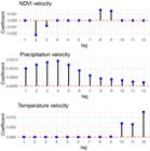
Representation of the velocity variables. The chart features three subplots, each illustrating the relationship between a coefficient and the lag for different variables. Additionally, each subplot includes bars that indicate the direction and effect of the lag variable. NDVI = normalized difference vegetation index; PREC = precipitation; TEMP = temperature.

Figure 9
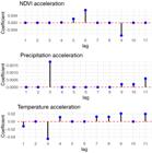
Representation of the acceleration variables. The chart features three subplots, each illustrating the relationship between a coefficient and the lag for various variables. Additionally, each subplot includes bars that indicate both the direction and effect of the lag variable. NDVI = normalized difference vegetation index; PREC = precipitation; TEMP = temperature.

Based on these analyses, we can assert that the velocities and accelerations of NDVI, PREC, and TEMP have a causal effect on agricultural yield. Since these causal relationships involve time lags, we can state that the relationship is in the Granger sense (Granger, 1969). It is essential to highlight that these causal relationships are absent in the original remote sensing variables; constructing the velocity and acceleration variables is required if such causal connections are to be established.

To compare predictive capacity following the identification of causal relationships between the remote sensing variables and agricultural yield, we chose to use the XGBoost model described in Eq. (14) and Eq. (15). This approach allowed us to capture the complex non-linear patterns between the predictor variables xi and the response variable yi. Given that XGBoost is a highly flexible non-parametric model, combined with the constraints posed by a small sample size, there is a risk of overfitting when relationships are spurious or synthetic. In this context, our construction of velocity and acceleration variables helped mitigate this risk, as these variables maintain causal relationships with our response variable.

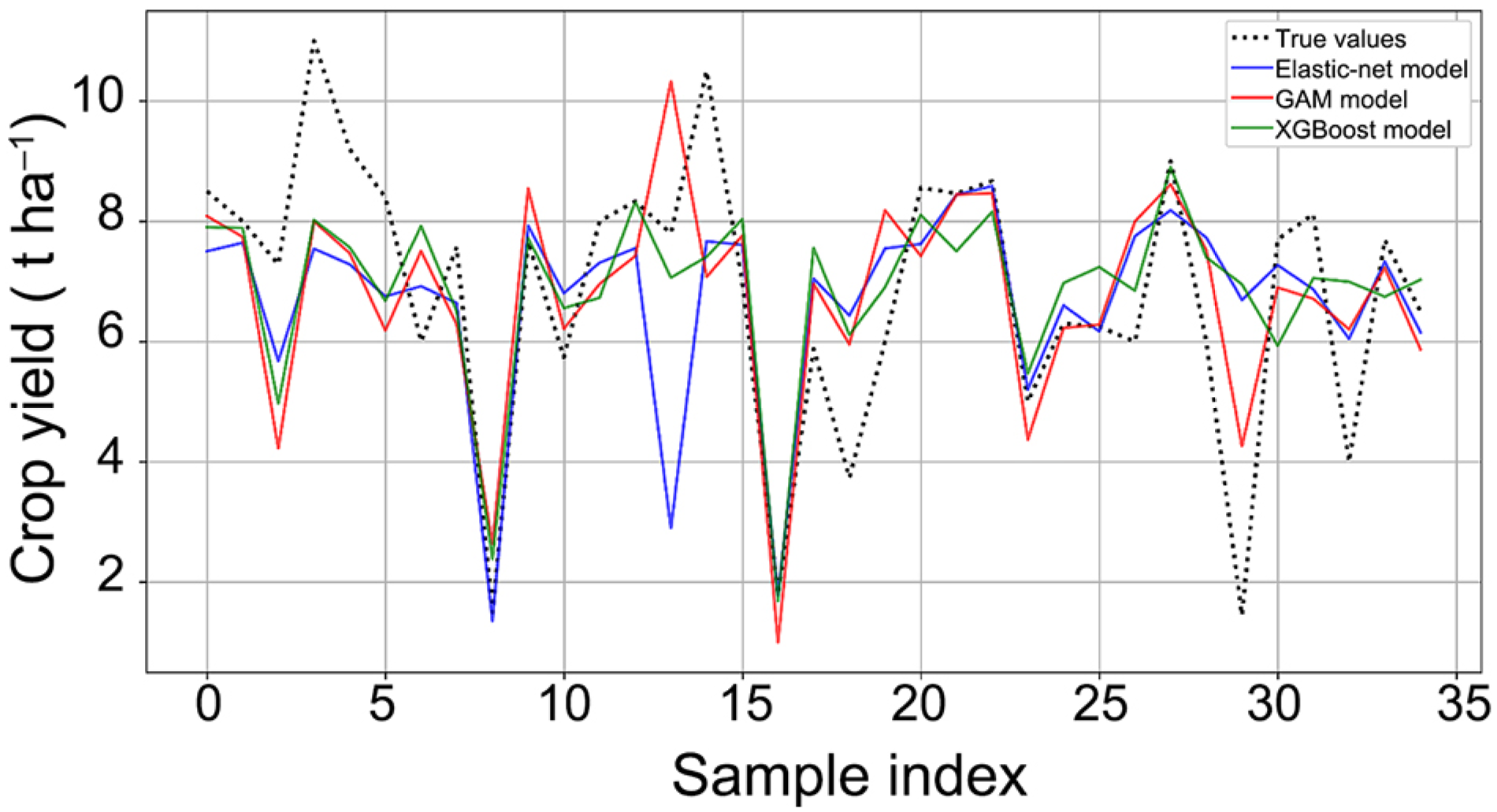
Since the Elastic-Net regularized regression model is fully parametric and XGBoost is completely non-parametric, we also included a semi-parametric alternative in our comparative prediction analysis: the GAM model described in Eq. (16). To compare the three models, the dataset was split into training and test sets in an 80 to 20 % ratio, respectively. The performance of each model in both samples is presented in Table 3. A comparison of predictions on the test dataset is provided for the three models evaluated: Elastic-Net, GAM, and XGBoost. The results indicate that all three models exhibit similar mean squared error (MSE) values, with results of 3.12, 2.54, and 2.83, respectively. However, the semi-parametric GAM model demonstrates superior generalization capability, effectively avoiding the overfitting observed in the other models. This advantage is attributed to its ability to capture non-linear patterns while maintaining interpretability. A detailed summary of model performance is presented in Table 3, and a graphical comparison between actual values and model predictions is illustrated in Figure 10.

Table 3
Mean Square Error (MSE) results for the three models applied to training and test data.

MSE Results for training and test data across models
Model	Train	Validation
Elastic-Net Regularization	2.34	3.12
XGBoost	0.21	2.83
GAM	1.85	2.54

• GAM = generalized additive models.

Figure 10
Comparison between the actual values of the test set and the predictions of the Elastic Net, Generalized Additive Models (GAM), and XGBoost models. The fit of each model to the actual data, expressed in t ha–^­­­¹, is observed, allowing for the evaluation of their accuracy and generalization capability.

Discussion

Several recent studies have highlighted the potential of remote sensing variables for predicting agricultural yield, with NDVI being particularly recognized as a key indicator of crop health (Lobell et al., 2015; You et al., 2017). Nevertheless, many of these approaches rely on average values or static indices, overlooking the temporal dynamics intrinsic to agroecological processes (You et al., 2017). In response, this study introduces a methodological shift centered on computing the velocities and accelerations of remote sensing variables such as NDVI, PREC, and TEMP. This strategy enables the tracking of temporal changes in satellite signals. It facilitates the identification of explicit causal relationships between these variables and crop yield, representing a significant advancement over traditional modeling approaches.

In this regard, the XGBoost model shows a good fit, as evidenced by its low MSE in training (0.21); however, the significant difference between its MSE in training and test sets (2.83) suggests potential overfitting. In contrast, the Elastic-Net regularized regression model exhibits a smaller increase in MSE values (2.34 in training and 3.12 in test), indicating greater stability and better generalization ability. Meanwhile, the GAM model, with an MSE of 1.85 in training and 2.54 in test, achieves the best balance between fit and generalization, outperforming the other two models in the test set.

Therefore, the performance of the three models may be related to the limited amount of data available in this study, which restricts XGBoost's ability to perform effective cross-validation and adequately capture the interactions between the variables and agricultural yield. In this context, a central contribution of the present study is the construction of VELNDVIt and ACCELNDVIt variables, derived from remote sensing data, whose causal nature allows for a significant improvement in the prediction of agricultural yield. In addition, we identified the types of dynamic transformations that should be applied to remote sensing variables to enable their effective use in predictive models, reinforcing the value of integrating this type of information with machine learning techniques. Therefore, the use of these transformations, along with machine learning methods, represents a promising strategy for developing simpler and more accurate predictive models, significantly enhancing forecasting capabilities in agriculture. Although rice is used as an example, the methods and conclusions of this study have broader applicability.

• Declaration of use of AI technologies
  We affirm that no AI technologies were used in the preparation of this manuscript.

Data availability statement

The data used in this study is publicly available in the GitHub repository: https://github.com/MCIES-DCIES-FIEECS-UNI/Sparsity-Regularization-and-Causality-in-Agricultural-Yield, ensuring transparency and reproducibility.

Some data used in this study were obtained from agricultural censuses conducted in Peru between 2015 and 2018, which provide detailed and updated information on agricultural practices and characteristics. These data were accessed through the Plataforma Nacional de Datos Abiertos, available at:https://datosabiertos.gob.pe/search/type/dataset?query=encuesta+nacional+agropecuaria&sort_by=changed&sort_order=DESC.

References

• Asmar E, Vahidnia MH, Rezaei M, Amiri E. 2024. Remote sensing-based paddy yield estimation using physical and FCNN deep learning models in Gilan province, Iran. Remote Sensing Applications: Society and Environment 34: 101199. https://doi.org/10.1016/j.rsase.2024.101199
  » https://doi.org/10.1016/j.rsase.2024.101199
• Baquerizo NC, Ventocilla EJV. 2022. Evaluation of machine learning algorithms in the classification of multispectral satellite images, case: Peruvian Amazon. Ciencia Latina 6: 4946-4963 (in Spanish, with abstract in English). https://doi.org/10.37811/cl_rcm.v6i1.1843
  » https://doi.org/10.37811/cl_rcm.v6i1.1843
• Breiman L, Friedman J, Olshen RA, Stone CJ. 1984. Classification and Regression Trees. 1ed. Chapman and Hall/CRC, New York, NY, USA. https://doi.org/10.1201/9781315139470
  » https://doi.org/10.1201/9781315139470
• Cao J, Zhang Z, Tao F, Zhang L, Luo Y, Zhang J, et al. 2021. Integrating multi-source data for rice yield prediction across china using machine learning and deep learning approaches. Agricultural and Forest Meteorology 297: 108275. https://doi.org/10.1016/j.agrformet.2020.108275
  » https://doi.org/10.1016/j.agrformet.2020.108275
• Chen T, Guestrin C. 2016. XGBoost: A Scalable Tree Boosting System. KDD ‘16, San Francisco, CA, USA. https://doi.org/10.1145/2939672.2939785
  » https://doi.org/10.1145/2939672.2939785
• Chung H-J, Cho A, Lim S-T. 2012. Effect of heat-moisture treatment for utilization of germinated brown rice in wheat noodle. LWT 47: 342-347. https://doi.org/10.1016/j.lwt.2012.01.029
  » https://doi.org/10.1016/j.lwt.2012.01.029
• Funk CC, Peterson PJ, Landsfeld MF, Pedreros DH, Verdin JP, Rowland JD, et al. 2014. A quasi-global precipitation time series for drought monitoring. U.S. Geological Survey, Reston, VA, USA. https://doi.org/10.3133/ds832
  » https://doi.org/10.3133/ds832
• Granger CWJ. 1969. Investigating causal relations by econometric models and cross-spectral methods. Econometrica 37: 424-438. https://doi.org/10.2307/1912791
  » https://doi.org/10.2307/1912791
• Guha S, Govil H, Diwan P. 2019. Analytical study of seasonal variability in land surface temperature with normalized difference vegetation index, normalized difference water index, normalized difference built-up index, and normalized multiband drought index. Journal of Applied Remote Sensing 13: 024518. https://doi.org/10.1117/1.JRS.13.024518
  » https://doi.org/10.1117/1.JRS.13.024518
• Hastie T, Tibshirani R, Wainwright M. 2015. Statistical Learning with Sparsity: the Lasso and Generalizations. p. 91-120. In: Hastie T, Tibshirani R, Wainwright M. eds. Generalizations of the Lasso Penalty. Chapman and Hall/CRC, Boca Raton, FL, USA. https://doi.org/10.1201/b18401
  » https://doi.org/10.1201/b18401
• Kussul N, Lavreniuk M, Skakun S, Shelestov A. 2017. Deep learning classification of land cover and crop types using remote sensing data. IEEE Geoscience and Remote Sensing Letters 14: 778-782. https://doi.org/10.1109/LGRS.2017.2681128
  » https://doi.org/10.1109/LGRS.2017.2681128
• Liakos KG, Busato P, Moshou D, Pearson S, Bochtis D. 2018. Machine learning in agriculture: a review. Sensors 18: 2674. https://doi.org/10.3390/s18082674
  » https://doi.org/10.3390/s18082674
• Liu Y, Pan Z, Zhuang Q, Miralles DG, Teuling AJ, Zhang T, et al. 2015. Agriculture intensifies soil moisture decline in Northern China. Scientific Reports 5: 11261. https://doi.org/10.1038/srep11261
  » https://doi.org/10.1038/srep11261
• Lobell DB, Thau D, Seifert C, Engle E, Little B. 2015. A scalable satellite-based crop yield mapper. Remote Sensing of Environment 164: 324–333. https://doi.org/10.1016/j.rse.2015.04.021
  » https://doi.org/10.1016/j.rse.2015.04.021
• Martínez B, Gilabert MA. 2009. Vegetation dynamics from NDVI time series analysis using the wavelet transform. Remote Sensing of Environment 113: 1823-1842. https://doi.org/10.1016/j.rse.2009.04.016
  » https://doi.org/10.1016/j.rse.2009.04.016
• Saunders RW, Kriebel KT. 1988. An improved method for detecting clear sky and cloudy radiances from AVHRR data. International Journal of Remote Sensing 9: 123-150. https://doi.org/10.1080/01431168808954841
  » https://doi.org/10.1080/01431168808954841
• Volante J, Mosciaro J, Morales Poclava M, Vale L, Castrillo S, Sawchik J, et al. 2015. Expansión agrícola en Argentina, Bolivia, Paraguay, Uruguay y Chile entre 2000-2010. Caracterización espacial mediante series temporales de índices de vegetación. Revista de Investigaciones Agropecuarias 41: 179-191 (in Spanish, with abstract in English).
• Wood SN. 2017. Smoothers. p. 221-275. In: Wood SN. ed. Generalized Additive Models: An Introduction with R. 2ed. Chapman and Hall/CRC, Boca Raton, FL, USA. https://doi.org/10.1201/9781315370279
  » https://doi.org/10.1201/9781315370279
• Wongsai N, Wongsai S, Huete AR. 2017. Annual seasonality extraction using the cubic spline function and decadal trend in temporal daytime MODIS LST data. Remote Sensing 9: 1254. https://doi.org/10.3390/rs9121254
  » https://doi.org/10.3390/rs9121254
• You J, Li X, Low M, Lobell DB, Ermon S. 2017. Deep Gaussian Process for Crop Yield Prediction Based on Remote Sensing Data. Proceedings of the AAAI Conference on Artificial Intelligence 31(1): 4559–4566. https://doi.org/10.1609/aaai.v31i1.11172
  » https://doi.org/10.1609/aaai.v31i1.11172
• Zou H, Hastie T. 2005. Regularization and variable selection via the elastic net. Journal of the Royal Statistical Society Series B: Statistical Methodology 67: 301-320. https://doi.org/10.1111/j.1467-9868.2005.00503.x
  » https://doi.org/10.1111/j.1467-9868.2005.00503.x

Edited by

• Edited by:
  Ricardo Enrique Bartosik https://orcid.org/0000-0002-0956-6081

Publication Dates

• Publication in this collection
  20 Apr 2026
• Date of issue
  2026

History

• Received
  26 Dec 2024
• Accepted
  20 Apr 2025