Comparative study between local and average constitutive models for reinforced concrete panels

Estudo comparativo entre modelos constitutivos locais e médios para painéis de concreto armado

Abstract

Abstract  This article presents a calculation procedure for the Cracked Membrane Model (CMM) using optimization techniques based on previous works. For this purpose, the proposed calculation routine is divided into two phases. The first phase consists of determining the initial estimation of the solution through a linear truss model with average stresses and strains, the Mohr Compatibility Truss Model (MCTM). In the second phase, an optimized calculation procedure to solve the system of nonlinear equations of the CMM is proposed, taking the solution of the MCTM as the initial estimate for the first iteration. The obtained solutions are compared with the experimental and numerical results found in the literature, where good accuracy and low computational cost were observed. Additionally, a comparative study is presented between average constitutive models (Rotating-Angle Softened Truss Model (RA-STM)), where the equilibrium is evaluated using average stresses, and local constitutive models (CMM), where the equilibrium is calculated at the crack. Focus was given to the steel reinforcement behavior at the crack. A modified Wood&Armer method was also used. The overall RC panels’ behavior predicted by RA-STM and CMM was close to the experimental results, including the failure stress. It is discussed the advantage of using local models in problems where the reinforcement maximum stress is of interest, such as fatigue problems and crack opening calculation. This paper aims to contribute to developing efficient strategies for modeling RC structures using local models, especially in design problems where the evaluation of the maximum reinforcement stress is fundamental.

Keywords:
membrane elements; reinforced concrete; constitutive models; optimization techniques; local behavior of the reinforcement

Resumo

Resumo  Este artigo apresenta um procedimento de cálculo para o Modelo de Membrana Fissurada (CMM) utilizando técnicas de otimização baseada em trabalhos anteriores. Para tanto, a rotina de cálculo proposta é dividida em duas fases. A primeira fase consiste em determinar a estimativa inicial da solução através de um modelo de treliça linear com tensões e deformações médias, o Modelo de Treliça de Compatibilidade de Mohr (MCTM). Na segunda fase, é proposto um procedimento de cálculo otimizado para resolver o sistema de equações não lineares do CMM, tomando a solução do MCTM como estimativa inicial para a primeira iteração. As soluções obtidas são comparadas com os resultados experimentais e numéricos encontrados na literatura, onde foram observadas boa precisão e baixo custo computacional. Adicionalmente, é apresentado um estudo comparativo entre modelos constitutivos médios (Rotating-Angle Softened Truss Model (RA-STM)), onde o equilíbrio é avaliado usando termos médios, e modelos constitutivos locais (CMM), onde o equilíbrio é avaliado na fissura. Foi dado enfoque ao comportamento da armadura de aço na fissura. Também foi utilizado o método Wood&Armer modificado. Os comportamentos gerais dos painéis RC previstos pelos RA-STM e CMM são próximos aos resultados experimentais, incluindo a tensão de ruptura. É discutida a vantagem da utilização de modelos locais em problemas onde a tensão máxima na armadura é de interesse, como problemas com fadiga e cálculo de abertura de fissuras. Este artigo visa contribuir para o desenvolvimento de estratégias eficientes para modelagem de estruturas de concreto armado utilizando modelos locais, especialmente em problemas de projeto onde a tensão máxima da armadura é fundamental.

Palavras-chave:
elementos de membrana; concreto armado; modelos constitutivos; técnica de otimização; comportamento local da armadura

1 INTRODUCTION

The formulation of the constitutive models used for the analysis of the structural behavior of reinforced concrete (RC) members depends on the problem to be solved, the accuracy required, and the concrete and steel behavior. In the case of concrete, the main focus is on the study of its compressive strength. The steel reinforcement, in its turn, resists the tensile forces after concrete cracking.

In structural engineering, RC elements that are designed to resist in-plane forces, such as deep beams, beam web and shear walls, can be evaluated by 2D membrane elements. In the literature, it is possible to find several models to simulate these types of elements, using, for example, plasticity, strut-and-tie and stress field models [¹]. During the last decades, truss models have proven to be adequate for such purposes, justifying their use to the present day, always aiming to improve the accuracy of the results and the numerical efficiency gain. The contributions of Vecchio and Collins [²] stand out among the various studies with truss models applied in the analysis of RC panels. They proposed correcting the stress-strain relationship for concrete in compression by incorporating the concrete softening effect and formulated the Compression Field Theory (CFT). Some years later, modifications were implemented by Vecchio and Collins [³] to mainly include the concrete average tensile stress capacity in the transverse direction of the concrete struts, proposing the Modified Compression Field Theory (MCFT). The consideration of tension stiffening was innovative, making MCFT the basis for later developed models.

Currently, two classes of constitutive models are identified to evaluate membrane elements, which are: average models in which the equilibrium is established in average terms of the stresses in the concrete and in the reinforcement (stresses in the materials are evaluated on average along a distance considering several cracks), and local models in which the equilibrium is established at the crack and as there is no concrete in that location, only the stress in the reinforcement is considered. The most widespread average constitutive models are the MCFT and the Softened Truss Model (STM), proposed by Hsu [⁴], later on being modified and renamed as the Rotating-Angle Softened Truss Model (RA-STM). In it, tension stiffening was incorporated using empirical constitutive laws. Posteriorly, alternative and efficient calculation procedures for models based on the RA-STM were proposed, in which the equations are solved using optimization algorithms, Silva [⁵], Silva et al. [⁶], Bernardo et al. [⁷], [⁸]. These works were relevant due to the computational efficiency demonstrated in relation to other literature works involving these models, whose solution is based simply on trial and error techniques, Greene [⁹], Hsu and Mo [¹⁰].

On the other hand, the most widespread local constitutive model is the Cracked Membrane Model (CMM), proposed by Kaufmann [¹¹]. The tension stiffening was incorporated using the theoretical formulation of the Tension Chord Model (TCM) [¹²]. In this, the stress in the reinforcement is evaluated at the crack, where equilibrium is being established. The original CMM formulation only considers the stabilized crack phase. Seelhofer [¹³] introduced an additional stress-strain relationship for steel to consider crack formation when slip exists. Alternatively, an analytical formulation of the crack spacing in closed form was proposed by Dabbagh and Foster [¹⁴].

The different approaches used by each model to evaluate the same aspect can lead to different predictions of the panel behavior. Depending on the mechanical conditions and purpose of the designer, a structural analysis based on average parameters may be sufficient to characterize its behavior. Nonetheless, in other design situations where, for example, the reinforcing steel stress is a crucial variable (fatigue problems), the stresses must be evaluated where maximum stresses occur, which is at the crack, as observed by Eshwarappa and Gangolu [¹⁵], and an average stresses analysis would not be suitable.

From the above, this article has two purposes: the development of an optimized CMM routine and to carrying out a comparative study of the structural analysis of RC panels subjected to membrane loads evaluated using the average constitutive model (RA-STM, Hsu [⁴], Bernardoet al. [¹⁶]) and the local model (CMM). The proposed CMM routine uses optimization techniques, based on the previous works from Silva [⁵] and Bernardo et al. [¹⁶], which until now have only been applied to average constitutive models. During the study, it was found that the implementation based on the original CMM (stabilized cracking) presented convergence problems, and the solution could not be found even in the initial loading phase. It has been overcome considering the formulations of Seelhofer [¹³], which also model the crack formation phase. The routine showed good accuracy when compared to experimental and numerical results in the literature, in addition to low computational cost (processing time close to 1 second for solving more than 2000 nonlinear systems of equations, corresponding to each point of the structure load-displacement behavior). In the comparative study, it was observed that both models were able to accurately evaluate the behavior of RC panels subjected to in-plane stresses. However, it was found that the stress in the reinforcement using the local constitutive model is higher than that obtained using the other model. The critical reinforcement stress is at the crack. Therefore, in problems associated with the critical steel behavior, such as fatigue, average values are not representative and are inadequate for evaluating the structure. The stress of the steel reinforcement was also calculated using a modified version of the well-known Wood&Armer method in order to verify its suitability in relation to the previous finding. This procedure is an adaptation of the classical analysis method of the internal forces for the design of RC plates, proposed by Wood [¹⁷] and Armer [¹⁸], applied to membrane elements and is presented in the structural software STRAP [¹⁹]. As will be shown in this paper, the modified Wood&Armer method was adequate to evaluate the maximum stresses in the steel reinforcement, in comparison to the average constitutive model.

Finally, it is expected that the routine presented will contribute to developing efficient strategies for modeling RC structures using local models, illustrating the importance of the crack formation phase not only for the physical modeling of the structure, but also for the procedure numerical stability. Furthermore, the discussion related to the comparative study between local and average models deals with an important subject in structural design practice, mainly regarding the behavior of the reinforcement in cases such as fatigue and crack opening evaluation, enabling the fulfillment of both service and ultimate analysis.

2 CRACKED MEMBRANE MODEL - CMM

The first objective of this work is covered in this section. Initially, a description of the CMM is made, which was proposed by Kaufmann [¹¹], and incorporates the effect of tension stiffening according to the TCM idealized by Marti et al. [¹²]. Finally, the procedures used to solve the CMM will be presented, culminating in the proposed algorithm. The abbreviations present in this work are described in Table 1.

Table 1
Abbreviations.

Abbreviation	Description	Abbreviation	Description
AS	Average stress	RA-STM	Rotating-Angle Softened Truss Model
CFT	Compression Field Theory	RC	Reinforced Concrete
CMM	Cracked Membrane Model	SC	Stress at the crack
MCFT	Modified Compression Field Theory	STM	Softened Truss Model
MCTM	Mohr Compatibility Truss Model	TCM	Tension Chord Model

2.1 Tension Chord Model - TCM

2.1.1 Tension stiffening

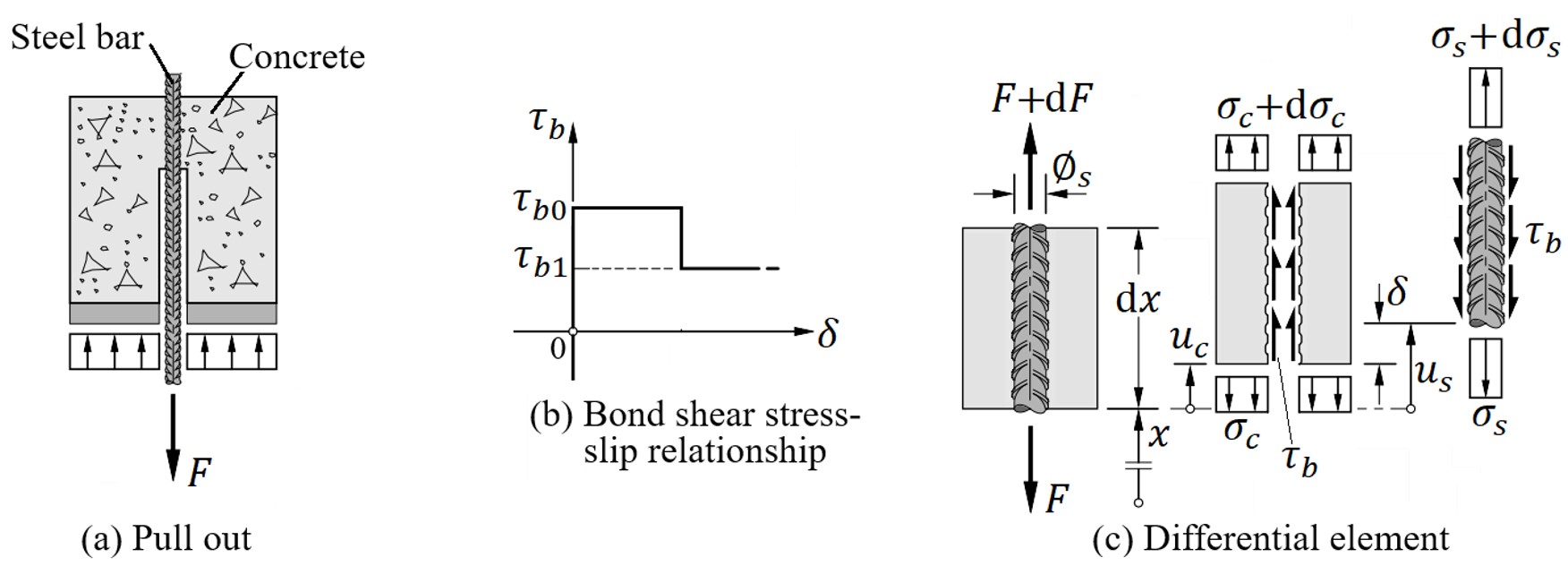
The combination of the characteristics of concrete and steel to gain structural strength is only possible when both are intimately connected by a mechanism called bond. The so-called slip bond results from different deformations between these materials, observed when the tensile deformations in the concrete are greater than the limit. When analyzing an infinitesimal element of length $dx$, Figure 1(c), from the pull-out test, Figure 1(a), subjected to a monotonic increasing force $F$, assuming a linear elastic behavior for steel (${\sigma }_s=E_s{\epsilon }_s)$ and concrete (${\sigma }_c=E_c{\epsilon }_c$), the equilibrium and compatibility conditions results in a second-order differential equation (shown in Equation 1), that relates the slip $\delta$ between reinforcement and concrete with the bond shear stress ${\tau }_b\left(x\right)$. The variables $E_s$ and $E_c$ are the Young’s modulus for steel and concrete, respectively, $n$ is their ratio and $\rho =A_s/A_c$, where $A_c$ is the concrete gross area and $A_s$ is the cross-section area of the steel bar, given by $\pi {{ø}_s}^2/4$. The nomenclature of the unknowns is described in Table 2.

Figure 1
Bond shear stress and tension stiffening.

Table 2
Nomenclature.

Notation	Description	Notation	Description
$A_c$ , $A_s$	concrete and reinforcement cross-section gross area	${\epsilon }_{sy},$ ${\epsilon }_{su}$	yielding and ultimate strain of steel
$E_c$ , $E_s$	concrete and steel Young’s modulus	${\epsilon }_x,$ ${\epsilon }_z$ , ${\gamma }_{xz}$	strains in plane $xz$
$E_{sh}$	steel hardening modulus	${\epsilon }_1$ , ${\epsilon }_3$	initial average strain in the $1$ and 3 directions
$f_c^{\text{'}}$	uniaxial compressive concrete strength	${\sigma }_{ctr}$, ${\sigma }_{cnr},$${\tau }_{ctnr}={\tau }_{cntr}$	concrete stresses at the crack
$f_c$	peak compressive stress	${\sigma }_c,$ ${\sigma }_s$	concrete and steel stress
$f_{ct}$	concrete tensile strength	${\sigma }_{sx},$ ${\sigma }_{sz}$	steel stress in the $x$ and $z$ direction
$f_{sy},$ $f_{su}$	steel yielding and ultimate stress	${\sigma }_{c3r}$	concrete compressive stress at the crack
$f_{sux},$ $f_{suz}$	steel ultimate stress in the $x$ and $z$ direction	${\sigma }_{cm}$, ${\sigma }_{sm}$	concrete and steel average stress
$F$	tensile force	${\sigma }_{s,min}$	steel minimum stress
$F_{CMM}^{\left(1\right)}$, $F_{CMM}^{\left(2\right)}$	first and second residual function for the CMM procedure	${\sigma }_{sm1},$ ${\sigma }_{sm2},$ ${\sigma }_{sm3}$	steel average stress in regimes 1, 2 and 3
$F_{MCTM}$	MCTM residual function	${\sigma }_{sr}$	steel stress at the crack
$F_x^{*}$ , $F_z^{*}$	reinforcement design forces in the $x$ and $z$ direction	${\sigma }_{sxr},$ ${\sigma }_{szr}$	steel stress at the crack in the $x$ and $z$ direction
$F_x$ , $F_z$ , $F_{xz}$	applied forces to the membrane element	${\sigma }_{sr1},$ ${\sigma }_{sr2},$ ${\sigma }_{sr3}$	steel stress at the crack in regimes 1, 2 and 3
$m_x,$$m_z$, $m_{xz}$	proportionality coefficients	${\sigma }_x$, ${\sigma }_z,$${\tau }_{xz}$	applied stresses in plane $xz$
$n$	Young’s modular ratio	${\sigma }_{c1}$	concrete tensile average stress
$s_{rm}$	crack spacing	${\sigma }_1$	principal tensile stress
$s_{rmx}$, $s_{rmz}$	crack spacing in the $x$ and $z$ direction	$\eta$	stresses ratio
$s_{rm0}$	maximum crack spacing	${ø}_s$	rebar diameter
$s_{rmx0}$, $s_{rmz0}$	maximum crack spacing in the $x$ and $z$ direction	${\theta }_r$	crack angle
$x_1,$ $x_2$	first and second transfer length	$\rho$	geometrical reinforcement ratio
$u_c,$ $u_s$	concrete and reinforcement displacements	${\rho }_x$ , ${\rho }_z$	geometrical reinforcement ratio in the $x$ and $z$ direction
$\delta$	slip	$\lambda$	ratio between crack spacing
${\epsilon }_{co}$	concrete strain corresponding to the peak stress	${\lambda }_x$ , ${\lambda }_z$	ratio between crack spacing in the $x$ and $z$ direction
${\epsilon }_c,$ ${\epsilon }_s$	concrete and steel strain	${\tau }_b$	bond shear stress
${\epsilon }_{sm}$	steel average strain	${\tau }_{b0}$, ${\tau }_{b1}$	bond shear stresses prior to and after the onset of reinforcement yielding
${\epsilon }_{sr}$	crack strain

$\frac{d^2\delta }{d{x}^2}=\frac{4{\tau }_b\left(x\right)}{{\mathrm{ø}}_s{E}_s}\left(\begin{array}{c}1-\frac{n\rho }{1-\rho }\end{array}\right)$ (1)

Sigrist [20] suggested a simplified solution for this equation, representing the bond stress as perfectly rigid-plastic, through a step function composed of two levels, Figure 1(b). Thus, the bond shear stress ${\tau }_b\left(x\right)$, is obtained with Equations 2 and 3. Where, ${\sigma }_s$ is steel stress, $f_{sy}$ is the yielding stress and $f_c^{\mathrm{\text{'}}}$ is the uniaxial compressive concrete strength in MPa.

${\tau }_{b0}=\mathrm{}0.6{f_c^{\mathrm{\text{'}}}}^{2/3}$ se ${\sigma }_s\le f_{sy}$(2)

${\tau }_{b1}=\mathrm{}0.3{f_c^{\mathrm{\text{'}}}}^{2/3}$se ${\sigma }_s>f_{sy}$(3)

The model of the bond stress as a function of the slip is applied in the evaluation of the steel stress at the crack, ${\sigma }_{sr}$, which is related to its steel average strain ${\epsilon }_{sm}$. The calculation of that stress depends on the so-called tension stiffening, which occurs due to the bond mechanisms, and causes an increase of the stiffness due to the contribution of the tensile concrete between cracks, Kvam [²¹].

2.1.2 Cracks spacing

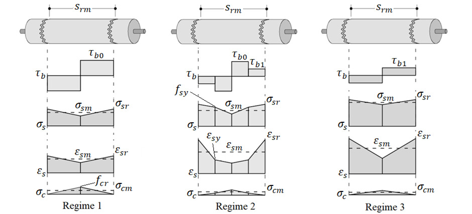
The cracks spacing in a tensile member, $S_{rm}$ (Figure 2), is limited to $S_{rm0}$, being the maximum cracks spacing corresponding to the situation where the concrete tensile stresses, transferred to concrete through bond, are equal to the tensile strength $f_{ct}$. Considering the bond stress-slip relationship proposed by Sigrist [²⁰] and the fact that the crack formation stage ends before the steel starts to yield, the bond stress is equal to ${\tau }_{b0}$. In this way, according to Marti et al. [¹²], the maximum crack spacing can be calculated according to Equation 4.

Figure 2
Distribution of stresses and strains in each regime.

$S_{rm0}=\frac{f_{ct}{\mathrm{ø}}_s}{2{\tau }_{b0}}\frac{(1-\rho )}{\rho }$ (4)

On the other hand, the cracks spacing cannot be inferior to $S_{rm0}$/2. For example, if the crack spacing is 40% of $S_{rm0}$, this means that a new crack developed in the middle of a length corresponding to 80% of the maximum crack spacing, which is inconsistent with the current model. The limitation imposed on the actual cracks spacing $S_{rm}$ can be summarized by the parameter $\lambda$ which corresponds to the ratio between the spacing between cracks $S_{rm}$ and the maximum spacing between cracks $S_{rm0}$, i.e., $\lambda =S_{rm}/S_{rm0}$. Its value, therefore, is defined in the interval $0.5\le \lambda \le 1$.

2.1.3 Stresses in steel and concrete

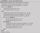
Since the bond stresses are represented by a step function with two domains (before and after steel yielding), the steel stress at the crack ${\sigma }_{sr}$ can fall into three distinct regimes: steel not yielded, steel partially yielded and steel fully yielded, Pimentel [²²], Figure 2.

If ${\sigma }_{sr}\le f_{sy}$ (Regime 1) the stress at the crack in regime 1 ${\sigma }_{sr1}$ is calculated with Equation 5.

${\sigma }_{sr1}={\sigma }_{sm1}+{\int }_{x=0}^{S_{rm}/4}d{\sigma }_s=E_s{\epsilon }_{sm}\mathrm{}+\frac{{\tau }_{b0}{S}_{rm}}{{\mathrm{ø}}_s}$ (5)

If ${\sigma }_{s,min}\le f_{sy}\le {\sigma }_{sr2}$ (Regime 2) the minimum stress ${\sigma }_{s,min}$ is calculated according to Sigrist [²⁰] by Equation 6, the stress at the crack in regime 2 ${\sigma }_{sr2}$ is calculated with Equation 7 and the steel average stress in regime 2 ${\sigma }_{sm2}$ is calculated from Equation 8, Kaufmann [¹¹]. Where $E_{sh}$ is the hardening modulus of steel, see section 2.2.4.

${\sigma }_{s,\mathrm{}min}={\sigma }_{sr2}-\left({\sigma }_{sr2}-f_{sy}\right)\left(1-\frac{{\tau }_{b0}}{{\tau }_{b1}}\right)-\frac{2{\tau }_{b0}{S}_{rm}}{{\mathrm{ø}}_s}$ (6)

${\sigma }_{sr2}=f_{sy}+2\frac{\frac{{\tau }_{b0}{S}_{rm}}{{\mathrm{ø}}_s}-\sqrt{(f_{sy}-E_s{\epsilon }_{sm})\frac{{\tau }_{b1}{S}_{rm}}{{\mathrm{ø}}_s}\left(\frac{{\tau }_{b0}}{{\tau }_{b1}}-\frac{E_s}{E_{sh}}\right)+\frac{E_s}{E_{sh}}{\tau }_{b0}{\tau }_{b1}\frac{{S_{rm}}^2}{{{\mathrm{ø}}_s}^2}}}{\frac{{\tau }_{b0}}{{\tau }_{b1}}-\frac{E_s}{E_{sh}}}$ (7)

${\sigma }_{sm2}=f_{sy}-\frac{{\left({\sigma }_{sr2}-f_{sy}\right)}^2{\mathrm{ø}}_s}{4{\tau }_{b1}{S}_{rm}}\left(\frac{{\tau }_{b0}}{{\tau }_{b1}}-1\right)+\left({\sigma }_{sr2}-f_{sy}\right)\frac{{\tau }_{b0}}{{\tau }_{b1}}-\frac{{\tau }_{b0}{S}_{rm}}{{\mathrm{ø}}_s}$ (8)

If $f_{sy}<{\sigma }_{s,min}$ (Regime 3) the stress at the crack in regime 3 ${\sigma }_{sr3}$ is calculated with Equation 9. The average steel stress in Regime 3, ${\sigma }_{sm3}$, is evaluated similarly to Regime 1.

${\sigma }_{sr3}={\sigma }_{sm3}+{\int }_{x=0}^{S_{rm}/4}d{\sigma }_s=f_{sy}+\left({\epsilon }_{sm}-\frac{f_{sy}}{E_s}\right)E_{sh}+\frac{{\tau }_{b1}{S}_{rm}}{{\mathrm{ø}}_s}$ (9)

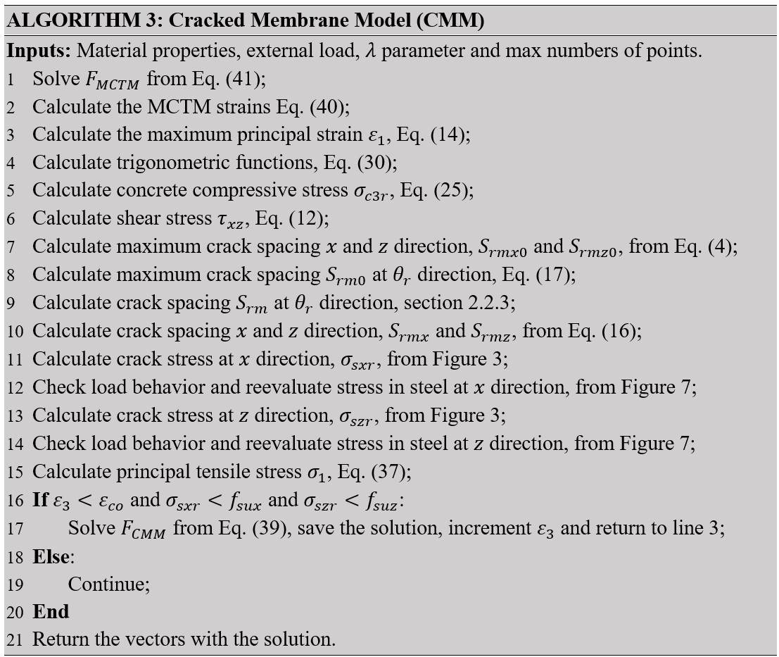
According to the discussions presented in this section, a computational routine was implemented in the Python language, as described in Figure 3.

Figure 3
TCM Pseudocode.

2.2 CMM Theory

The CMM is used for the structural analysis of RC panels under in-plane or membrane forces. The CMM satisfies the three principles of structural mechanics, which are: forces equilibrium, deformation compatibility and constitutive relationships for the materials.

2.2.1 Equilibrium equations

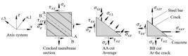
Figure 4(a) presents a 2D RC member reinforced in the orthogonal directions, and under membrane forces in the $x-z$ plane, namely: normal stresses ${\sigma }_x$ and ${\sigma }_z$, and shear stress ${\tau }_{xz}$=${\tau }_{zx}$. The cracks in the concrete are parallel to each other and evenly spaced, with an angle ${\theta }_r$ to the $x$ axis. In this model, this angle is considered variable. Longitudinal and transverse steel bars are parallel to the $x$ and $z$ axes, respectively.

Figure 4
Cracked membrane model.

In the CMM, the equilibrated state in the member is defined at the crack without stresses in concrete, Figure 4(b). Consequently, the normal stress ${\sigma }_{cnr}$ and the shear stresses ${\tau }_{ctnr}$and ${\tau }_{cntr}$ are zero. Given these assumptions and according to Figure 4(b), the concrete contribution can be represented by the compressive normal stress ${\sigma }_{ctr}$, oriented according to the coordinate system of the principal stresses $n-t$.

For the reinforcement, since the Dowell effect is neglected (the steel bars do not resist shear stresses). Its contribution is considered through the normal stresses ${\sigma }_{sxr}$ and ${\sigma }_{szr}$ in the $x$ and $z$ directions, respectively. By performing the coordinate transformation between the $x-z$ coordinate system of the applied in-plane stress state and the $n-t$ principal coordinate system, the 2D member equilibrium, Figure 4(b), is obtained as presented in Equations 10, 11 and 12, [¹¹]. The term ${\sigma }_{ctr}$ is renamed as ${\sigma }_{c3r}$.

${\sigma }_x={\rho }_x{\sigma }_{sxr}+{\sigma }_{c3r}{cos}^2{\theta }_r$ (10)

${\sigma }_z={\rho }_z{\sigma }_{szr}+{\sigma }_{c3r}{sin}^2{\theta }_r$ (11)

${\tau }_{xz}=-{\sigma }_{c3r}sin{\theta }_{r}cos{\theta }_r$ (12)

2.2.2 Deformation compatibility

The deformation compatibility conditions can be obtained from the Mohr’s circle for strains. By performing the coordinate transformation between the $x-z$ coordinate system of the applied in-plane stress state and the $n-t$ principal coordinate system, it is possible to obtain three relationships, Equation 13 [²³], which relate the average normal strains (${\epsilon }_x$, ${\epsilon }_z$) and shear strains ${\gamma }_{xz}$ with the average principal tensile and compressive strains (${\epsilon }_1$ and ${\epsilon }_3$). The $1-3$ axis system is the same as the $n-t$ system.

$\left[\begin{array}{c}{\epsilon }_x\\ {\epsilon }_z\\ {\gamma }_{xz}\end{array}\right]=\left[\begin{array}{ccc}{cos}^2{\theta }_r& {sin}^2{\theta }_r& sin{\theta }_{r}cos{\theta }_r\\ {sin}^2{\theta }_r& {cos}^2{\theta }_r& -sin{\theta }_{r}cos{\theta }_r\\ -2sin{\theta }_{r}cos{\theta }_r& 2sin{\theta }_{r}cos{\theta }_r& {cos}^2{\theta }_r-{sin}^2{\theta }_r\end{array}\right]\left[\begin{array}{c}{\epsilon }_3\\ {\epsilon }_1\\ 0\end{array}\right]$ (13)

From the matrix equation Equation 13, the so-called first invariant for strains is obtained, as shown in Equation 14. This relationship can be used to evaluate the average principal tensile strain ${\epsilon }_1$ based on the average strains ${\epsilon }_3$, ${\epsilon }_x$ and ${\epsilon }_z$.

${\epsilon }_1+{\epsilon }_3={\epsilon }_x+{\epsilon }_z$ (14)

From the compatibility equations a relation between the crack angle and the average strains is obtained [¹¹] as presented in Equation 15.

${{tan}^2\theta }_r=\frac{{\epsilon }_x-{\epsilon }_3}{{\epsilon }_z-{\epsilon }_3}$ (15)

2.2.3 Cracks spacing in RC panels

The cracks spacing along the direction of the reinforcement is obtained through a trigonometric relation between the oblique cracks spacing $S_{rm}$ and crack direction ${\theta }_r$. Thus, Equation 16 indicates the spacing between cracks ($S_{rmx}$, $S_{rmz}$) in x and z directions. For an in-plane stress state, the parameters ${\lambda }_x=S_{rmx}/S_{rmx0}$ and ${\lambda }_z=S_{rmz}/S_{rmz0}$ can assume values beyond the predetermined interval for the uniaxial stress state.

$S_{rmx}=\frac{S_{rm}}{sin{\theta }_r};\mathrm{}{S}_{rmz}=\frac{S_{rm}}{cos{\theta }_r}$ (16)

The oblique cracks spacing $S_{rm}$, according to Kaufmann [¹¹], is described as discussed for the case of a 1-D member, Section 2.1.2. Therefore, the necessary conditions for the formation of new cracks are similar. Thus, $S_{rm}$ is a function of its maximum spacing, i.e., $S_{rm}=\lambda S_{rm0}$, with the parameter $\lambda$ varying in the interval $0.5\le \lambda \le 1.$ The maximum cracks spacing $S_{rm0}$ in a cracked panel corresponds to the situation in which the principal tensile stress ${\sigma }_1$ in the member, in the middle point between cracks, is equal to the concrete tensile strength $f_{ct}$. As suggested by Dabbagh and Foster [¹⁴], one can obtain $S_{rm0}$, Equation 17. The variables in this equation are calculated using Equations 18, 19, 20, 21 and 22.

$S_{rm0}=\frac{a+\eta b-\sqrt{\eta c+d+{S_{rmz0}}^2+{\eta }^2({S_{rmx0}}^2-d)}}{2}$ (17)

With:

$\eta =\left|{\tau }_{xz}\right|/f_{ct}$ (18)

$a=S_{rmx0}sin\left|{\theta }_r\right|+S_{rmz0}cos\left|{\theta }_r\right|$ (19)

$b=S_{rmx0}cos\left|{\theta }_r\right|+S_{rmz0}sin\left|{\theta }_r\right|$ (20)

$c=2\left({S_{rmx0}}^2+{S_{rmz0}}^2\right)sin\left|{\theta }_r\right|cos\left|{\theta }_r\right|-2S_{rmx0}{S}_{rmz0}$ (21)

$d=\left({S_{rmx0}}^2-{S_{rmz0}}^2\right){sin}^2\left|{\theta }_r\right|-2S_{rmx0}{S}_{rmz0}sin\left|{\theta }_r\right|cos\left|{\theta }_r\right|$ (22)

2.2.4 Materials constitutive models

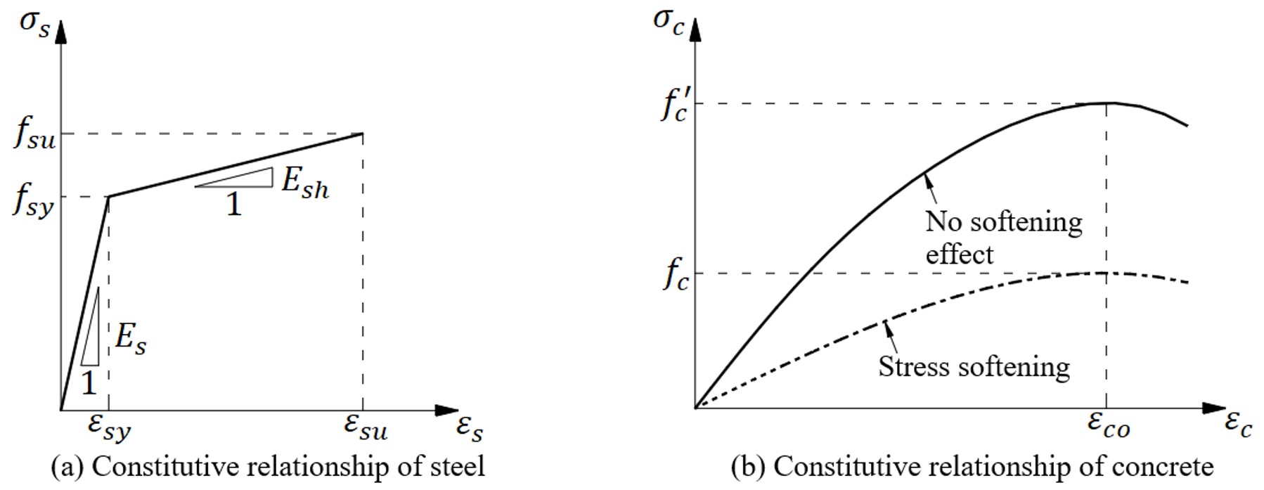
The behavior of the steel bars is modeled considering only the capacity of resisting axial forces, neglecting the dowel effect. For simplicity, Sigrist [²⁰] proposed an approximated constitutive relationship for steel, described by a bilinear stress-strain graph, as illustrated in Figure 5(a).

Figure 5
Constitutive relationships.

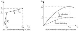
In this model, the stress-strain is represented by two lines with distinct directions whose inflection point is the yielding stress $f_{sy}$. In the elastic stage (first line segment), the proportionality constant is the longitudinal Young’s modulus, $E_s$, while, in the plastic stage (second line segment), it is the hardening modulus $E_{sh}$, obtained by Equation 23, considering ${\epsilon }_{su}$ the ultimate strain, $f_{su}$ the ultimate stress and ${\epsilon }_{sy}$ yielding strain of steel.

$E_{sh}=\frac{f_{su}-f_{sy}}{{\epsilon }_{su}-{\epsilon }_{sy}}$ (23)

The model for the compressive concrete behavior is based on the stress-strain response of a cylindrical specimen under uniaxial loading. In this case, the response is approximated by a parabola, as illustrated in Figure 5(b). As the member under study is subjected to a biaxial stress state, the compressive concrete strength obtained from uniaxial testing is no longer representative. According to Kaufmann [¹¹], in cracked concrete panels, the so-called softening effect of concrete is observed, which arises due to the tensile strains ${\epsilon }_1$perpendicular to the compressive concrete direction, and consequently reduces the compressive concrete strength. To consider this effect in the model, Kaufmann [¹¹] proposed a correction only for the strength (stress softening), making an adjustment based on the tensile strain ${\epsilon }_1$. This correction is made through Equation 24, where $f_c$ is the corrected compressive concrete strength in MPa.

$f_c=\frac{{{(f}_c^{\mathrm{\text{'}}})}^{2/3}}{0.4+30{\epsilon }_1}\le f_c^{\mathrm{\text{'}}}$ (24)

Thus, the stress-strain relationship in the concrete in the pre-peak stage is described by Equation 25, Kaufmann [¹¹], and illustrated in Figure 5(b), where ${\epsilon }_{co}$ is the strain corresponding to the peak stress.

${\sigma }_{c3r}=f_c\frac{{\epsilon }_3^2+2{\epsilon }_3{\epsilon }_{co}}{{\epsilon }_{co}^2}$ (25)

2.2.5 Behavior for low loading level

The CMM implemented routine, based on the discussions thus far, encountered convergence issues in the solution in the initial phase of the load/deformation analysis, as the relationships are based on the assumption of stabilized cracking. For low loading levels (when the slip does not occur throughout the entire member length), the CMM overestimates the tension stiffening when determining the distance between the fictitious cracks. This causes incompatibilities in the steel strains and stresses and, consequently, inaccuracy in the solution of the system of equations of the model [¹³].

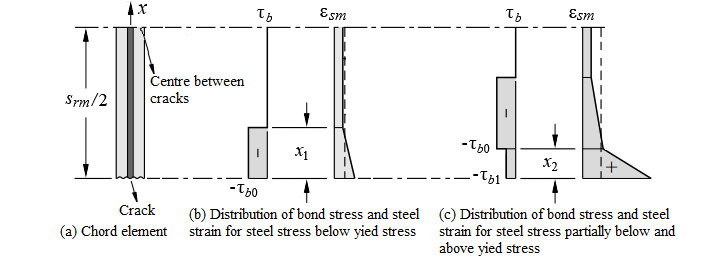
This problem was not originally considered by Kaufmann [¹¹] when conceptualizing the CMM. In this work, the response for low loading levels was obtained according to an adaptation of the CMM presented by Seelhofer [¹³] and Kvam [²¹]. In this model, the slip between the materials is only considered near the crack, Figure 6. Thus, if the slip for steel before yielding $x_1$ is less than $S_{rm}/2$, Equation 26, Figure 6(b), and ${\sigma }_{sr}\le f_{sy}$, then the stress ${\sigma }_{sr}$ is obtained by Equation 27.

Figure 6
Behavior for low loading level.

$x_1=\frac{S_{rm}}{2}\left(\sqrt{n^2{\rho }^2+\frac{E_s{\epsilon }_{sm}}{{\tau }_{b0}}\frac{{\mathrm{ø}}_s}{S_{rm}}}-n\rho \right)$

$0\le x_1\le S_{rm}/2$ (26)

${\sigma }_{sr}=x_1\frac{4{\tau }_{b0}}{{\mathrm{ø}}_s}(1+n\rho )$ (27)

Otherwise, if ${\sigma }_{sr}\ge f_{sy}$ and the slip for the yielded steel $x_2$, obtained by Equation 28, is in the interval $0\le x_2\le S_{rm}/2$, Figure 6(c), then it is used Equation 29. With $\alpha$ equal to $1+n\rho$.

$x_2=\frac{{\mathrm{ø}}_s{f}_{sy}{E}_{sh}}{4{\tau }_{b1}\alpha E_s}\left\{\sqrt{1+4\alpha \frac{E_s}{E_{sh}}\left[\frac{S_{rm}{\tau }_{b1}}{{\mathrm{ø}}_s{f}_{sy}}\left(\frac{\alpha E_s{\epsilon }_{sm}}{f_{sy}}-n\rho \right)-\frac{{\tau }_{b1}}{4{\tau }_{b0}\alpha }\right]}-1\right\}$ (28)

${\sigma }_{sr}=f_{sy}+x_2\frac{4{\tau }_{b1}}{{\mathrm{ø}}_s}$ (29)

The subroutine corresponding to the behavior for low loading levels is described in Figure 7. It is performed after the steel stresses have been determined using the TCM model, Figure 3.

Figure 7
Low loading level behavior pseudocode.

2.3 Implemented algorithm for the Cracked Membrane Model (CMM)

2.3.1 Additional equations

From the compatibility equations Equation 13, and from trigonometric identities, it is possible to define two additional equations relating the cracking angle ${\theta }_r$ of the RC panel with the strains in the $x-z$ and $1-3$ system, as demonstrated by Hsu and Mo [¹⁰]. These equations are Equation 30.

${sin}^2{\theta }_r=\frac{{\epsilon }_x-{\epsilon }_3}{{\epsilon }_1-{\epsilon }_3};\mathrm{}{cos}^2{\theta }_r=\frac{{\epsilon }_z-{\epsilon }_3}{{\epsilon }_1-{\epsilon }_3}$ (30)

These equations are relevant for models where the angle ${\theta }_r$ varies, such as CMM. They eliminate this angle from the equilibrium equations, enhancing numerical stability in the solution procedure, Silva [⁵]. In the CMM, they were also used to calculate $S_{rm}$.

2.3.2 Proportional loading

In the analysis of the stress-strain response of the CMM, the applied stresses (${\sigma }_x$, ${\sigma }_z$, ${\tau }_{xz}$) can be related to the concrete principal tensile stress ${\sigma }_1$ Equation 32, through proportionality coefficients, as described by Hsu and Mo [¹⁰] and shown in Equation 31.

$m_x=\frac{{\sigma }_x}{{\sigma }_1};\mathrm{}{m}_z=\frac{{\sigma }_z}{{\sigma }_1};\mathrm{}{m}_{xz}=\frac{{\tau }_{xz}}{{\sigma }_1}$ (31)

${\sigma }_1=\frac{{\sigma }_x+{\sigma }_z}{2}+\sqrt{{\left(\frac{{\sigma }_x-{\sigma }_z}{2}\right)}^2+{{\tau }_{xz}}^2}$ (32)

Replacing Equation 31 in the equilibrium equations Equations 10, 11 and 12, one obtains Equations 33, 34 and 35.

$m_x{\sigma }_1-{\rho }_x{\sigma }_{sxr}={\sigma }_{c3r}{cos}^2{\theta }_r$ (33)

$m_z{\sigma }_1-{\rho }_z{\sigma }_{szr}={\sigma }_{c3r}{sin}^2{\theta }_r$ (34)

$m_{xz}{\sigma }_1=-{\sigma }_{c3r}sen{\theta }_{r}cos{\theta }_r$ (35)

The product of Equations 33 and 34 results in Equation 36.

$\left(m_x{\sigma }_1-{\rho }_x{\sigma }_{sxr}\right)\left(m_z{\sigma }_1-{\rho }_z{\sigma }_{szr}\right)={{(m}_{xz}{\sigma }_1)}^2$ (36)

The solution of the previous equation defines a new relationship for the stress ${\sigma }_1$, Equation 37. The parameter B is calculated as shown in Equation 38.

${\sigma }_1=\frac{1}{2(m_x{m}_z-{m_{xz}}^2)}(B\pm \sqrt{B^2-4\left(m_x{m}_z-{m_{xz}}^2\right)\left({\rho }_x{\sigma }_{sxr}{\rho }_z{\sigma }_{szr}\right)}$ (37)

$B=m_z{\rho }_x{\sigma }_{sxr}+m_x{\rho }_z{\sigma }_{szr}$ (38)

Based on this loading configuration, the equations Equations 33 and 34 constitute the system of nonlinear equations Equation 39, which is solved during the solution procedure of the proposed routine.

$\left\{\begin{array}{c}{F}_{CMM}^{\left(1\right)}={\rho }_x{\sigma }_{sxr}+{\sigma }_{c3r}{cos}^2{\theta }_r-m_x{\sigma }_1=0\\ F_{CMM}^{\left(2\right)}={\rho }_z{\sigma }_{szr}+{\sigma }_{c3r}{sin}^2{\theta }_r-m_z{\sigma }_1=0\end{array}\right.$ (39)

Similarly to Silva [⁵], in the solution procedure, the chosen variables were normalized values of the average strains ${\epsilon }_x$ and ${\epsilon }_z$.

2.3.3 Initial estimation (Mohr Compatibility Truss Model - MCTM)

To start the computational optimization tools used to compute the response of the system of equations, an initial estimation is required. Depending on it, the solver can provide or not acceptable results, or even fail to converge to any solution. For RC members, such as cracked membrane elements, one possibility is to use a simple model, assuming a linear behavior for the materials [⁵].

Therefore, assuming linear and elastic materials, the equilibrium equations of the membrane element, as described in section 2.2.1, can be rewritten as Equation 40,

${\epsilon }_x=\frac{m_x+m_{xz}cot{\theta }_r}{{E_s\rho }_x}{\sigma }_1;\mathrm{}{\epsilon }_z=\frac{m_z+m_{xz}tg{\theta }_r}{{E_s\rho }_z}{\sigma }_1;\mathrm{}{\epsilon }_3=\frac{{-m}_{xz}}{E_{c}sin{\theta }_{r}cos{\theta }_r}{\sigma }_1$ (40)

For an elastic analysis, equation Equation 15 can be solved using Equation 42. This approach is called the Mohr Compatibility Truss Model (MCTM), Hsu and Mo [¹⁰]. The resulting equation is nonlinear, Equation 41, and the angle ${\theta }_r$ is the unknown to be obtained.

$F_{MCTM}={tan}^2{\theta }_r-\frac{{\epsilon }_x-{\epsilon }_3}{{\epsilon }_z-{\epsilon }_3}=0$ (41)

To solve Equation 41 in the implemented routine, the nonlinear equation optimization tool is adopted, using the principal stress angle as an initial estimation. With the solution, the strains ${\epsilon }_x$, ${\epsilon }_z$, and ${\epsilon }_3$ are determined by Equation 40. These, in turn, are used as initial estimation to solve the nonlinear system of equations in the CMM.

2.3.4 Implementation of the CMM algorithm

Based on the discussion of the CMM model, a computational routine described in Figure 8 was implemented. The routine is divided into two phases: MCTM and CMM.

Figure 8
CMM Pseudocode.

The first phase involves determining the initial estimation of the strains from the solution Equation 41. In the second phase, corresponding to the CMM, the system of nonlinear equations, Equation 39, is solved by taking the MCTM strains as the initial point for the first iteration. To solve this problem, the fsolver function from the Scipy library, Scipy Community [²⁴], implemented in the Python language, was used. This tool proved to be efficient, enabling a fast evaluation and offering a robust algorithm. For the analysis of the load-deformation response of the member, this routine can be performed several times by incrementing the strain ${\epsilon }_3$, and by using the previous CMM solution as the initial estimation for solving the new CMM system of nonlinear equations. This process is repeated until the defined number of points is reached or the strain ${\epsilon }_3$ exceeds the specified limit or, alternatively, if any reinforcement reaches the failure stress.

3 CODE VALIDATION

In this section, the validation of the discussed algorithm for the TCM and CMM models will be shown, by comparing it with experimental and numerical results from the literature.

3.1 Validation of the computational implementation of TCM

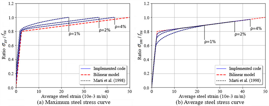
The implementation of the TCM was validated through a problem studied by Marti et al. [¹²], which evaluates the stresses ${\sigma }_{sr}$ and ${\sigma }_{sm}$ as a function of the strain ${\epsilon }_{sm}$. The concrete properties are: $f_c^{\text{'}}=30\mathrm{M}\mathrm{P}\mathrm{a}$ and $E_c=10{f_c^{\text{'}}}^{1/3}\mathrm{G}\mathrm{P}\mathrm{a}$. The cracks spacing is equal to $S_{rm}=S_{rm0}$ ($\lambda =1$). The steel properties are: $f_{sy}=500\mathrm{M}\mathrm{P}\mathrm{a}$, $f_{su}=625\mathrm{M}\mathrm{P}\mathrm{a}$, $E_s=205\mathrm{G}\mathrm{P}\mathrm{a}$, ${\epsilon }_{su}=50\times {10}^{-3}$, and ${ø}_s=16\mathrm{m}\mathrm{m}$. The analyzes are made for reinforcement ratios $\rho$ equal to 1%, 2% and 4%. The Figure 9 show the results. To build the curves, the increased variable was the average strain in the reinforcement.

Figure 9
TCM analysis results.

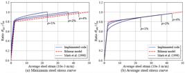
According to Figure 9, one can observe that the results from the computational implementation, based on the routine of Figure 3, agree with those documented in the literature. Besides, it is worth mentioning that, in the development of the curves using the TCM, a strain increment of 0.02‰ was considered (which corresponds to approximately 2300 points evaluated, until the ultimate strain is reached). Considering all the 2300 points, the processing time remained below 1 second. It demonstrates the efficiency of this routine.

3.2 Validation of the computational implementation of the CMM

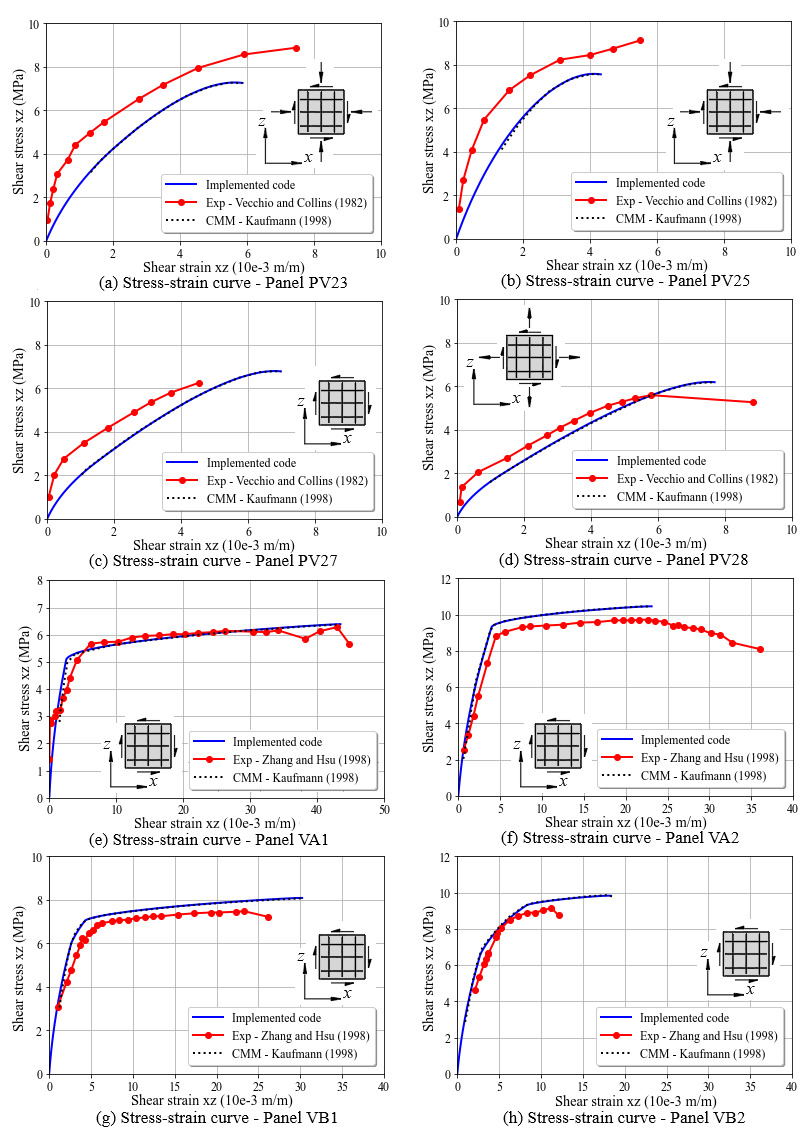
The implementation of the CMM was validated with the experimental results of 12 RC panels orthogonally reinforced and tested under in-plane stresses. These panels are named by series as presented by the authors, namely: Marti and Mayboom [²⁵] for series PP; Vecchio and Collins [²] for series PV; and Zhang and Hsu [²⁶] for series VA and VB. The dimensions of the panels are: PP series equal to 162.6$\times$162.6$\times$28.7 cm, PV series equal to 89$\times$89$\times$7 cm and VA and VB series equal to 139.7$\times$139.7$\times$17.8 cm. The material properties and the applied loading (also indicated in each figure) are depicted in Table 3. The Young’s modulus of the reinforcements is $E_s=200\mathrm{G}\mathrm{P}\mathrm{a}$. The analysis considered the spacing between oblique cracks calculated with $\mathrm{\lambda }=1$ and the convergence tolerance of fsolver was 10e-8. The PP1, PV27 panels and the VA and VB series were tested in a pure shear state in the $x-z$ plane. In turn, panels PV23, PV25 and PV28 were subjected to normal and shear stresses, with the ratio between normal stress and shear stress equal to -0.39, - 0.69 and +0.32. The validation results are shown in Figures 10 and 11. In PP1 the curves ${\tau }_{xz}-{\gamma }_{xz}$, ${\tau }_{xz}-$ ${\epsilon }_1$, ${\tau }_{xz}$ $-$ ${\epsilon }_3$ and ${\tau }_{xz}$ $-$ ${\theta }_r$ were evaluated, while for the others only the curve ${\tau }_{xz}$ $-$ ${\gamma }_{xz}$ was evaluated. A comparison is also made with the original numerical solution of the CMM, according to Kaufmann [¹¹], and with the numerical solution obtained by implementing Kvam [²¹] (CMM also considering the crack formation phase [¹³], [¹⁴]).

Table 3
Basic data for panel analysis.

Panel	Reinforcement										Concrete		La
	${\rho }_x$	${ø}_x$	$f_{syx}$	$f_{sux}$	${\epsilon }_{sux}$	${\rho }_z$	${ø}_z$	$f_{syz}$	$f_{suz}$	${\epsilon }_{suz}$	$f_c^{\text{'}}$	${\epsilon }_{co}$
	%	mm	MPa	MPa	‰	%	mm	MPa	MPa	‰	MPa	‰
PP1	1.942	19.5	479	667	90	0.647	11.3	480	640	91	27.0	2.12	PSb
PV23	1.785	6.35	518	596	100	1.785	6.35	518	596	100	20.5	2.00	-0.39c
PV25	1.785	6.35	466	536	100	1.785	6.35	466	536	100	19.3	1.80	-0.69c
PV27	1.785	6.35	442	508	100	1.785	6.35	442	508	100	20.5	1.90	PSb
PV28	1.785	6.35	483	555	100	1.785	6.35	483	555	100	19.0	1.85	+0.32c
VA1	1.143	11.3	445	579	100	1.143	11.3	445	579	100	95.1	2.45	PSb
VA2	2.276	16.0	409	534	100	2.276	16.0	409	534	100	98.2	2.50	PSb
VB1	2.28	16.0	409	534	100	1.14	11.3	445	579	100	98.2	2.50	PSb
VB2	3.42	19.5	455	608	100	1.14	11.3	445	579	100	97.6	2.45	PSb
A2	1.19	-	463	464	10	1.19	-	463	464	10	41.2	2.10	PSb
A3	1.79	-	446	447	10	1.79	-	446	447	10	41.6	1.94	PSb
A4	2.98	-	470	471	10	2.98	-	470	471	10	42.5	2.20	PSb

• ªExternal load applied to the panel; ^bPure shear; ^cRatio between stresses ${\sigma }_x/\left|{\tau }_{xz}\right|={\sigma }_z/\left|{\tau }_{xz}\right|$

Figure 10
Analysis of the panel PP1.

Figure 11
Analysis of the panels from PV, VA and VB-series.

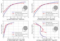
In general, good agreement can be observed between the results obtained from the computational implementation and those documented in the literature. In the PP1 panel, when compared with the numerical solution of Kvam [²¹], both solutions coincide along the entire curve (Figure 10). For the PV, VA, and VB series panels, shown in Figure 11, Kaufmann [¹¹] did not present the numerical estimations for the solution.

Given the good routine prediction, it appears that the MCTM approach as an auxiliary tool to obtain an initial estimation, previously applied in average constitutive models, is also usable for local constitutive models. It also avoids using trial and error techniques, adopted by other authors [⁹], [¹⁰]. Furthermore, it was observed that convergence issues occurred in the initial stage when analyzing the RC membranes using the author's original formulation. This occurs because the formulation was proposed considering stabilized cracking. To mitigate these issues, Seelhofer [¹³] formulations for low loading levels (section 2.2.5) were incorporated, as was done by Kvam [²¹], to adjust the stress in the steel for low-stress levels, which was not initially considered in the CMM model. It proved to be important not only for the physical model precision, as considered by the authors mentioned above, but it was also identified that it plays a relevant role from a numerical point of view, enabling gains in numerical stability and improving the convergence of the solution in the transition from the uncracked to the cracked stage. It is worth mentioning that, when considering the development of a load-displacement curve with 1000 points (1000 systems of nonlinear equations), the processing time did not exceed 1 second, demonstrating its efficiency. Comparisons of processing time were not possible, as none of the authors indicated the curve processing time.

4 COMPARATIVE STUDY BETWEEN AVERAGE AND LOCAL MODELS

This section presents the analysis and discussions related to the comparative study between the average and local constitutive models. In the first one, the equilibrium of the membrane element is considered in terms of the average values of both the concrete and the steel, as indicated in section AA in Figure 12. On the other hand, in the second model, the equilibrium is satisfied at the crack (local), according to the BB cut in Figure 12, as there is no concrete in that location; only the stress in the reinforcement is considered. To carry out this study, the predictions of orthogonally reinforced RC panels were compared using the average constitutive model RA-STM by Hsu [⁴], adopted by Silva [⁵], Silva et al. [⁶], and Bernardoet al. [¹⁶], and the local constitutive model CMM, which was implemented in this work and validated as shown in section 3. In addition, in RA-STM, tension stiffening is verified through empirical constitutive laws, while CMM uses the Tension Chord Model (TCM) [¹²].

Figure 12
Scheme of local and average constitutive models.

The RC panels evaluated are those from Series A tested by Pang and Hsu [²⁷]. They have dimensions of 140$\times$140$\times$17.8 cm and are subject to a state of pure shear in the $x-z$ plane. The reinforcement and concrete properties of each panel are described in Table 3, while the Young’s modulus of the reinforcement is $E_s=200\mathrm{G}\mathrm{P}\mathrm{a}$. The following properties were not provided by the author: ultimate stress, ultimate strain, and diameter of the bars. However, given the need to know the ultimate stress since the CMM model adopts a bilinear stress-strain relationship with hardening for the steel, the ultimate stress was adopted to be slightly greater than the yielding stress (as the model does not allow these two parameters to be the same), and the corresponding strain was 10‰, as prescribed in the Brazilian standard ABNT NBR 6118 [²⁸]. As for the diameter, despite being a necessary input data, it was verified that for panels with symmetrical reinforcement and pure shear loading type, equal to the ones of the Series A, the rebar diameter is not important to the model. Hence, an arbitrary value was adopted solely for the purpose of code execution. In the case of the solution via the CMM, the panels were evaluated for the two limit cases related with the spacing between oblique cracks, i.e., for $\lambda =0.5$ and $\lambda =1$.

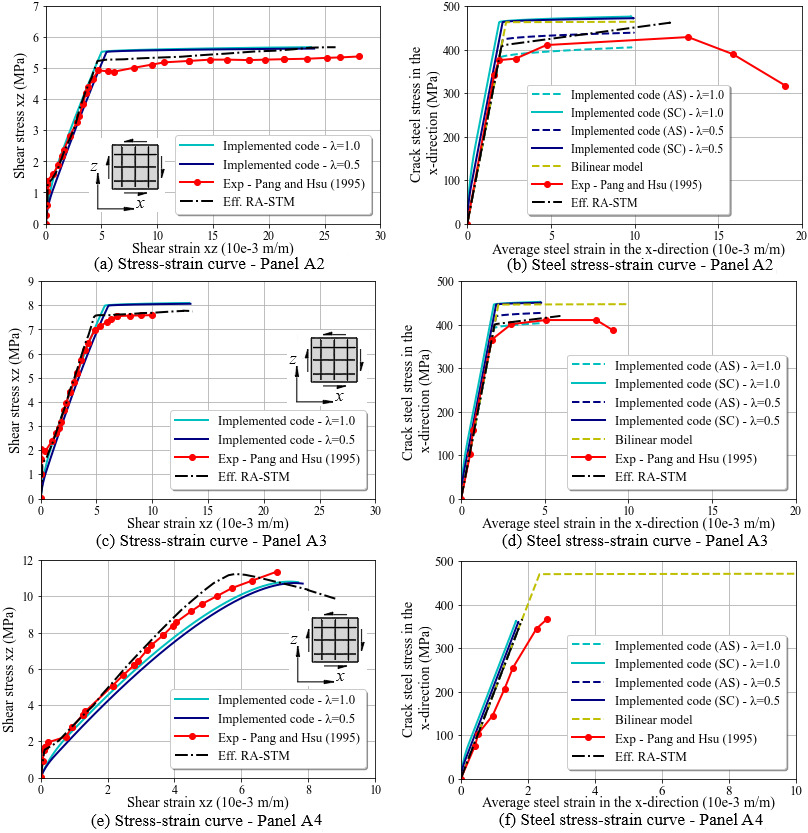
Figures 13(a), 13(c), and 13(e) illustrate the ${\tau }_{xz}$ $-$ ${\gamma }_{xz}$ curves from the constitutive models and from the experiments. Overall, the curves of both models show good agreement with the experimental data. Panels A2 and A3 yield predictions that closely align with almost all the curve paths, especially in the region corresponding to the service load (the region where the curve is approximately linear). After steel yielding, the average constitutive model (Eff. RA-STM) showed a higher level of agreement with the experimental results, while the local constitutive model (CMM) predicted a relatively higher stress for both values of $\lambda$. However, the failure stress of both models was practically the same. According to Kaufmann [¹¹], the panel can show higher stiffness when the equilibrium is locally established, i.e., at the crack. In panel A4, although the two models' predictions are representative when compared to the experiments, a higher variation is observed between the results, with the average model predicting a stiffer response. In predicting the behavior for low loading level, the Eff. RA-STM demonstrated a higher level of proximity to the experimental results in the transition point from the uncracked to the cracked stage. The CMM exhibits a smoother behavior in this region, such that no discontinuity is observed in the transition between these stages as for the other models.

Figure 13
Analysis of the panel A-series.

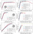
Figures 13(b), 13(d) and 13(f) show the average (AS) and local stress (SC) behavior versus average strain in the steel. For the CMM, the curves corresponding to both average and local stress are presented for $\lambda$ equal to 0.5 and 1. In the experiment and for the Eff. RA-STM model, the stress is equivalent to only the average. In Figures 13(b), 13(d), and 13(f), in terms of average values for the stresses in the reinforcement, there is a good correspondence between the two models and the experimental data before the yielding of the reinforcement. Both models (CMM e Eff. RA-STM) show very similar responses for panels A3 and A4 (especially considering $\lambda =1$).

However, Eff. RA-STM proved to be slightly stiffer when the steel yielded. In Figures 13(b) and 13(d), corresponding to panels A2 and A3, one can observe a failure by yielding of the reinforcement. The reinforcement ratio for those panels is lower than that of panel A4. This can be observed for the reinforcement in both directions, as they have the same properties. On the other hand, panel A4 Figure 13(f) presents a failure by concrete crushing without reinforcement yielding.

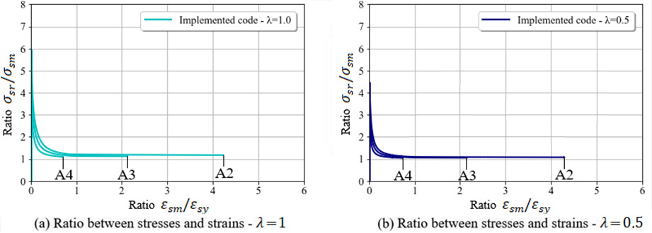
It is also observed that all the curves referring to the steel stress at the crack determined with the local constitutive model (CMM), as expected, presented a stress higher than the corresponding average value, regardless of the used model (CMM or Eff. RA-STM), or the value of λ. The highest stress value is evaluated with the maximum spacing between cracks calculated with λ = 1, which is in accordance with Spathelf [²³]. The steel stress at the crack is higher than the average stress, even for service loading when the reinforcement is not yielded. This fact can be observed from the Figure 14, which shows the relationship between ${\sigma }_{sr}/{\sigma }_{sm}$ and ${\epsilon }_{smx}/{\epsilon }_{sy}$, evaluated for the reinforcement along the x direction, considering the concrete post-cracking behavior. In all panels it is noted that the stress ratio (${\sigma }_{sr}/{\sigma }_{sm})$ is higher than 1, especially in the region before the yielding of the reinforcement (${\epsilon }_{sm}/{\epsilon }_{sy}<1)$. The reinforcement stress at the crack is also stiffer than the bilinear model, Figure 13(b), 13(d), and 13(f), which characterizes the steel not embedded in concrete, as discussed in Buchaim [²⁹].

Figure 14
Analysis of the panels from A-series.

The steel stress at the crack is higher than the corresponding average stress. This is consistent with what Eshwarappa and Gangolu [¹⁵] observed in cyclic loading tests, where the reinforcement failed exactly at the crack. In this way, it shows that the critical reinforcement stress occurs at the crack and constitutive models whose equilibrium is defined at the crack, as the CMM, are more suitable to evaluate it, although there are models that attempt to convert steel average stress into maximum steel stress at crack, Vecchio [³⁰]. Thus, in cases directly associated with the maximum behavior of the steel, such as crack opening calculation, or even in fatigue problems, it is known that the stress adopted for such cases must be the highest possible, i.e., at the crack. Therefore, average stresses are inadequate for such analysis.

In this comparative study, a modified version of the Wood&Armer Method was also considered. The original model was proposed by Wood [¹⁷] and Armer [¹⁸] and consists of determining the design moments in RC slabs considering the existence of bending and torsional moments. In this work, the approach implemented in the commercial software STRAP [¹⁹], was used. In this software, an adaptation is implemented that enables the method to be used to obtain the stresses in the reinforcements of RC membranes. As described in its user manual, for orthogonal reinforcements, the design forces in the reinforcement $F_x^{*}$ and $F_z^{*}$, along the $x$ and $z$ directions, respectively, are calculated according to Equation 42, with $F_x$ and $F_z$ being the normal forces, and $F_{xz}$ the shear force, in units of force per meter.

$F_x^{\mathrm{*}}=F_x+{|F}_{xz}|$ and $F_z^{\mathrm{*}}=F_z+{|F}_{xz}|$(42)

Besides, if $F_x^{*}$<0, the design forces in the reinforcement are calculated using Equation 43.

$F_x^{\mathrm{*}}$=0 and $F_z^{\mathrm{*}}=F_z+\left|\frac{{F_{xz}}^2}{F_x}\right|$(43)

Alternatively, if $F_z^{*}$<0, the design forces in the reinforcement are calculated using Equation 44.

$F_z^{\mathrm{*}}$=0 and $F_x^{\mathrm{*}}=F_x+\left|\frac{{F_{xz}}^2}{F_z}\right|$(44)

Finally, once the design forces in the reinforcement are known, the steel stresses can be calculated through Equation 45, with $F_x^{*}$ and $F_z^{*}$ given in units of force per meter.

${\sigma }_{sx}=\frac{F_x^{\mathrm{*}}}{{\rho }_x{A}_c}$ and ${\sigma }_{sz}=\frac{F_z^{\mathrm{*}}}{{\rho }_z{A}_c}$(45)

As series A panels were submitted to a pure shear state, the design stresses of the reinforcement, obtained by the modified Wood&Armer equations, were based only on the shear force. As in this model, the external loads are resisted exclusively by the reinforcement, the material corresponding response in Figure 13 coincides with the bilinear model, which, as can be seen, had good proximity to the CMM maximum stresses.

Thus, it can be concluded that the modified Wood&Armer method aligns with the perception that the critical stress is at the crack, therefore proving to be suitable for evaluating such stresses when compared to the other models discussed in this study.

5 CONCLUSIONS

In this article, a computational implementation of the Cracked Membrane Model using optimization techniques was presented. Additionally, a comparative study was conducted using average and local constitutive models employed for analyzing the behavior of RC membrane elements, specifically focusing on the Eff. RA-STM and the CMM. The code validation and comparative study were conducted through experimental and numerical results from panels available in the literature. Based on this, it can be concluded that:

1. The computational implementation demonstrated to be capable of accurately evaluating the behavior of RC membrane elements, especially the concrete response at the cracked stage with or without the reinforcement yielded. The MCTM proves to be useful as an initial estimate for solving the system of equations for local constitutive models. The addition of the formulation for low load levels proved to be important not only for the physical model precision, as considered by other authors, but it was also relevant from a numerical point of view. Gains in numerical stability and improvements in the convergence of the solution in the transition from the uncracked to the cracked stage were observed, allowing the evaluation of 1000 points on the CMM stress-strain curve in less than 1 second.

2. Both constitutive models proved to be capable of accurately evaluating RC panels' behavior under in-plane stresses. In the shear stress-strain curve of panels A2 and A3, the average constitutive model (Eff. RA-STM) presented a better prediction after yielding while the local constitutive model (CMM) predicted a relatively higher stress. The opposite occurred on the A4 panel, with the average model being stiffer than the local one. A good prediction of the average stresses of the steel was obtained with the two models (especially before the reinforcement yielding). The reinforcement stress at the crack obtained using CMM was higher than the average stress in all the studied panels. This shows that the use of average steel stresses is inadequate for evaluating the reinforcement stress in problems where the maximum stress is critical, such as the case of steel fatigue;

3. The modified Wood&Armer method showed good results in evaluating the stresses for the reinforcement at the crack when compared to the CMM. This method proves to be an alternative methodology, especially in problems where the main focus is on the stress at the crack (as mentioned, for fatigue problems).

• Financial support:
  Postgraduate scholarship awarded by the Pernambuco Science and Technology Support Foundation (FACEPE)
• Data Availability:
  The data that support the findings of this study are available from the corresponding author, B. C. Fernandes, upon reasonable request.
• How to cite:
  B. C. Fernandes, J. R. B. Silva, B. Horowitz, and L. F. A. Bernardo, “Comparative study between local and average constitutive models for reinforced concrete panels,” Rev. IBRACON Estrut. Mater., vol. 18, no. 2, e18205, 2025, https://doi.org/10.1590/S1983-41952025000200005

REFERENCES FORMATS

• ¹ U. Häussler-Combe, Computational Methods for Reinforced Concrete Structures, Berlin: Ernst & Sohn, 2015.
• ² F. J. Vecchio and M. P. Collins, The Response of Reinforced Concrete to In-Plane Shear and Normal Stresses, Toronto: University of Toronto, Dept. of Civil Engineering, 1982.
• ³ F. J. Vecchio and M. P. Collins, “The modified compression-field theory for reinforced concrete elements subjected to shear,” ACI Eng., vol. 83, pp. 219–231, 1986, http://dx.doi.org/10.14359/10416
  » http://dx.doi.org/10.14359/10416
• ⁴ T. T. C. Hsu, “Softened truss model theory for shear and torsion,” ACI Eng., vol. 85, pp. 624–635, 1988, http://dx.doi.org/10.14359/2740
  » http://dx.doi.org/10.14359/2740
• ⁵ J. R. B. Silva, “Procedimento eficiente para análise de seções em concreto armado usando o modelo de treliça com amolecimento,” M.S. thesis, Dept. Civil Eng., Federal Univ. Pernambuco (UFPE), Recife, PE, Brazil, 2016.
• ⁶ J. R. B. Silva, B. Horowitz, and L. F. A. Bernardo, “Efficient analysis of beam sections using softened truss model,” ACI Struct. J., vol. 114, pp. 765–774, 2017, http://dx.doi.org/10.14359/51689568
  » http://dx.doi.org/10.14359/51689568
• ⁷ L. F. A. Bernardo, B. M. D. Cerquido, J. R. B. Silva, and B. Horowitz, “Efficient Refined rotating-angle softened truss model procedure to analyze reinforced concrete membrane elements,” Struct. Concr., vol. 19, pp. 1971–1982, 2018, https://doi.org/10.1002/suco.201800012
  » https://doi.org/10.1002/suco.201800012
• ⁸ L. F. A. Bernardo, A. R. B. Lyrio, J. R. B. Silva, and B. Horowitz, “Refined softened truss model with efficient solution procedure for prestressed concrete membranes,” J. Struct. Eng., vol. 144, pp. 144–146, 2018, http://dx.doi.org/10.1061/(ASCE)ST.1943-541X.000204
  » http://dx.doi.org/10.1061/(ASCE)ST.1943-541X.000204
• ⁹ G. G. Greene Jr, “Behavior of reinforced concrete girders under cyclic torsion and torsion combined with shear: experimental investigation and analytical models,” Ph.D. Dissertation, Department of Civil Engineering, University of Missouri, Rolla, USA, 2006.
• ¹⁰ T. T. C. Hsu and Y. L. Mo, “Unified Theory of Concrete Structures,” USA: Wiley, 2010.
• ¹¹ W. Kaufmann, “Strength and deformations of structural concrete subjected to in-plane shear and normal forces,” PhD Thesis, Institute of Structural Engineering, Swiss Federal Institute of Technology Zurich (ETHZ), Zurich, Switzerland, 1998.
• ¹² P. Marti, M. Alvarez, W. Kaufmann, and V. Sigrist, “Tension chord model for structural concrete. structural engineering international,” Struct. Eng. Int., vol. 8, pp. 287–298, 1998, http://dx.doi.org/10.2749/101686698780488875
  » http://dx.doi.org/10.2749/101686698780488875
• ¹³ H. Seelhofer, “Ebener Spannungszustand im Betonbau: Grundlagen und Anwendungen,” M.S. thesis, Institute of Structural Engineering, Swiss Federal Institute of Technology Zurich (ETHZ), Zurich, Switzerland, 2009.
• ¹⁴ H. Dabbagh and S. J. Foster, “A smeared fixed - crack model for the FE analysis of RC membranes incorporating aggregate interlock,” Adv. Struct. Eng., vol. 9, pp. 91–102, 2006, http://dx.doi.org/10.1260/136943306776232927
  » http://dx.doi.org/10.1260/136943306776232927
• ¹⁵ N. H. Eshwarappa and A. R. Gangolu, “Fatigue behavior of lightly reinforced concrete beams in flexure due to overload,” in 9th International Conference on Fracture Mechanics of Concrete and Concrete Structures, V. Saouma, J. Bolander, E. Landis, Eds, pp. 1–12, 2016, http://dx.doi.org/10.21012/FC9.042
  » http://dx.doi.org/10.21012/FC9.042
• ¹⁶ L. F. A. Bernardo, B. M. V. C. Filho, and B. Horowitz, “Refinement of the rotating-angle softened truss model with efficient solution procedure for RC membranes,” Eng. Struct., vol. 213, pp. 1–12, 2020, http://dx.doi.org/10.1016/j.engstruct.2020.110552
  » http://dx.doi.org/10.1016/j.engstruct.2020.110552
• ¹⁷ R. H. Wood, “The reinforcement of slabs in accordance with a predetermined field of moments,” Concrete (Lond.), vol. 2, pp. 69–76, 1968.
• ¹⁸ G. S. T. Armer, “Correspondence,” Concrete (Lond.), vol. 2, pp. 319–320, 1968.
• ¹⁹ ATIR Engineering Software Development, STRAP structural analysis programs 2021. STRAP user’s manual 2021. Available: https://atirsoft.com/strap-manual/ (accessed Apr. 15, 2023).
  » https://atirsoft.com/strap-manual/
• ²⁰ V. Sigrist, “Zum Verformungsvermögen von Stahlbetonträgern,” M.S. thesis, Institutfür Baustatikund Konstruktion, ETH, Zürich, Switzerland, 1995. (In German)
• ²¹ S. Kvam, “Implementation of the cracked membrane model for crack width predictions in reinforced concrete shell Structures,” MSc Dissertation, Department of Structural Engineering, Norwegian University of Science and Technology (NTNU), Norway, 2018.
• ²² M. J. S. Pimentel, “Numerical modelling for safety examination of existing concrete bridges,” Ph.D. dissertation, Faculty Eng., Univ. Porto (U. Porto), Porto, Portugal, 2011.
• ²³ C. A. Spathelf, “Fatigue performance of orthogonally reinforced concrete slabs,” Ph.D. dissertation, Institute of Structural Engineering, Swiss Federal Institute of Technology Zurich (ETHZ), Zurich, Switzerland, 2017.
• ²⁴ Scipy Community, “SciPy.optimize: scientific optimization in Python.” https://docs.scipy.org/doc/scipy/reference/optimize.html (accessed Apr. 15, 2023).
  » https://docs.scipy.org/doc/scipy/reference/optimize.html
• ²⁵ P. Marti and J. Meyboom, “Response of prestressed concrete elements to in-plane shear forces,” ACI Struct. J., vol. 89, pp. 503–514, 1992, http://dx.doi.org/10.14359/2956
  » http://dx.doi.org/10.14359/2956
• ²⁶ L. X. Zhang and T. T. C. Hsu, “Behavior and analysis of 100 MPa concrete membrane elements,” J. Struct. Eng., vol. 124, pp. 24–34, 1998, http://dx.doi.org/10.1061/(ASCE)0733-9445(1998)124:1(24)
  » http://dx.doi.org/10.1061/(ASCE)0733-9445(1998)124:1(24)
• ²⁷ X. B. Pang and T. T. C. Hsu, “Behavior of reinforced concrete membrane elements in shear,” ACI Struct. J., vol. 92, pp. 665–679, 1995, http://dx.doi.org/10.14359/9661
  » http://dx.doi.org/10.14359/9661
• ²⁸ Associação Brasileira de Normas Técnicas, Projeto de Estruturas de Concreto, ABNT NBR 6118, 2014.
• ²⁹ R. Buchaim, “A influência da não-linearidade física do concreto armado na rigidez à flexão e na capacidade de rotação plástica,” Ph.D. dissertation, Polytechnic School of Engineering, University of São Paulo (USP), São Paulo, Brazil, 2001.
• ³⁰ F. J. Vecchio, “Disturbed stress field model for reinforced concrete: formulation,” J. Struct. Eng., vol. 126, pp. 1070–1077, 2000, http://dx.doi.org/10.1061/(ASCE)0733-9445(2000)126:9(1070)
  » http://dx.doi.org/10.1061/(ASCE)0733-9445(2000)126:9(1070)

Edited by

• Editors:
  Osvaldo Manzoli, Daniel Cardoso.

Data availability

The data that support the findings of this study are available from the corresponding author, B. C. Fernandes, upon reasonable request.

Publication Dates

• Publication in this collection
  14 Feb 2025
• Date of issue
  2025

History

• Received
  24 Sept 2023
• Reviewed
  07 Jan 2024
• Accepted
  27 Feb 2024