Dynamic analysis of railway bridges incorporating soil-structure interaction

Análise dinâmica de pontes ferroviárias incorporando a interação solo-estrutura

Abstract

Abstract  This paper presents a dynamic analysis of a reinforced concrete railway bridge in northern Brazil, built in 1980, under the passage of heavy-haul railway vehicles. A parameterized geometric model of the bridge was developed using Rhino/Grasshopper, and a programming routine was implemented on GiD to automate the pre-processing modeling stage and generate outputs compatible with different FEM solvers. The dynamic analysis was then performed, accounting for the soil-structure interaction to reproduce the modes and natural frequencies of the analyzed asset. The computational model was calibrated and validated using modal identification results obtained from a structural health monitoring campaign. The validated model formed the basis for assessing the structural resilience of the bridge, indicating promising results regarding adopting the proposed modeling strategy.

Keywords:
soil-structure interaction; finite element method; railway bridges; dynamic analysis; resilience

Resumo

Resumo  Este artigo apresenta uma análise dinâmica de uma ponte ferroviária de concreto armado no norte do Brasil, construída em 1980, submetida à passagem de veículos ferroviários de grande carga. Um modelo geométrico parametrizado da ponte foi desenvolvido utilizando o ambiente Rhino/Grasshopper, e uma rotina de programação foi implementada no GiD para automatizar o pré-processamento e gerar saídas compatíveis com diferentes programas FEM. A análise dinâmica foi realizada considerando a interação solo-estrutura, de modo a reproduzir os modos e frequências naturais do ativo ferroviário, sendo o modelo computacional calibrado e validado com base nos resultados de identificação modal obtidos a partir de uma campanha de monitoramento estrutural do ativo. O modelo validado serviu de base para a avaliação da resiliência estrutural da ponte, indicando resultados promissores ao se empregar a estratégia de modelagem proposta.

Palavras-chav: interação solo-estrutura; método dos elementos finitos; pontes ferroviárias; análise dinâmica; resiliência

1 INTRODUCTION

Railway bridges are fundamental infrastructure assets for sustaining a country economy, whether to transport people or commodities. Throughout their life-cycle, these structures experience deterioration processes that lead to reduced performance and an increased risk of hazards. Therefore, assessing the structural condition of these assets is crucial to ensure secure operational integrity [¹], [²].

The structural dynamic response, a crucial aspect of railway bridges, is directly related to structure, foundation, and soil interaction [³]. A dynamic soil-structure analysis must ensure compatibility regarding these elements to represent the dynamic effects generated by external actions [⁴]. In this context, research frequently proposes various methods to apply the interaction between soil confinement and foundations, especially considering their influence on the natural frequency of vibration modes [⁵].

The dynamic behavior of bridge infrastructure is undoubtedly affected by specific soil-structure interaction (SSI) laws for deep [⁶] or shallow foundations [⁴]. König et al. [⁷] demonstrated that the damping provided by SSI significantly influences the structural behavior in resonance conditions when using vehicle-bridge interaction models. In this sense, an efficient methodology is sought to represent the effects of the soil and foundation interaction on the asset dynamic behavior to achieve computational responses that closely approximate the actual structure behavior when subjected to vehicle loads.

Several techniques are proposed in the literature to simulate the dynamic behavior of bridges using the SSI technique. One of these techniques simplifies the superstructure domain in unifilar finite elements and the foundation and soil for surface elements [⁸]. This type of strategy allows for consideration of the vehicle-bridge interaction and the imperfections generated by traffic. These aspects affect the dynamic behavior of the railway bridge based on the type of irregularity present on the tracks and the design characteristics of the railway compositions, translated through masses, springs, and dampers [⁷].

Another compelling approach is the use of volumetric finite elements associated with linear springs to represent the soil and its properties, producing frequency responses and vibration modes that allow for the evaluation of the importance of the SSI technique for bridge dynamic behavior [⁵]. Other possible strategies to consider the interaction between soil, foundation, and structure refer to methods based on the plasticity theory applied to unstructured finite element meshes and nonlinear physical soil behaviors [⁹]. This approach can be applied to small assets, such as pedestrian bridges; however, the sophistication of soil constitutive models makes it difficult to use this strategy for large bridges due to the high computational demands.

Regularly, impedance functions coupled with springs and dampers have been successfully used to represent the interaction processes between soil and foundation [¹⁰]. This type of strategy has shown satisfactory results for railway bridges supported on soils with different compactness [¹¹]. In other applications, such as seismic analyses of railway bridges, two-dimensional finite elements can be combined in unstructured meshes with springs and dampers to compose the constitutive solution in the asset infrastructure region [¹²]. Recent works have employed impedance functions representing soil stiffness foundations discretized in solid finite elements, considering soils with different mechanical properties [¹³].

For railway bridges supporting high-speed trains, linear springs with impedance functions have presented essential advances in understanding the effects of free vibrations for variations in railway composition speed and soil mechanical parameters [¹⁴]. Additionally, research has demonstrated the importance of considering the impact of SSI in structures focused on urban monorail transport [¹⁵].

Over the years, research into structures has focused on searching for coupled solutions between computational models and support for developing digital twins of civil engineering assets [¹⁶]. Such definitions are essential for railway bridges as they guarantee functionality according to the conditions of service and operation, reducing traffic interruptions for occasional repairs and reinforcements [¹⁷]. Additionally, structural resilience models depend on the dynamic responses of railway bridges, which can be obtained by computational models calibrated using instrumentation and monitoring data [¹⁸]. This makes it possible to determine structural resilience from a computational model calibrated to asset resilience based on multiple damage scenarios [¹⁹], [²⁰].

This paper proposes a computational modeling strategy for the dynamic analysis of railway infrastructure employing a soil-structure interaction (SSI) approach. For this, a properly calibrated Winkler spring model was employed to portray the combined effects of the structure-foundation-soil system and its material properties. The numerical model was calibrated and validated according to experimental responses from a monitoring campaign. The influence of SSI models was investigated by comparing the computational results concerning natural frequencies, vibration modes, accelerations, and velocities with experimental data, assessing the bridge structural response under dynamic loads.

Furthermore, the study introduces a parameterized geometric modeling approach and the automation of the pre-processing process for model generation through script implementation, which enhances modeling efficiency and facilitates adaptation to different scenarios that may be encountered in the bridge, such as structural modifications, damage assessments, or variations in material properties and boundary conditions. Finally, structural resilience was evaluated for the case study railway bridge, which opens new horizons for quantitatively assessing bridge components under unusual degradation events, repair timelines, and recovery efficiency.

The main contributions of this article include the evaluation of a soil-structure interaction approach to assess the dynamic behavior of a reinforced concrete railway bridge, advancements in the production of parameterized geometric models, the automation of the numerical model pre-processing step, and the quantification of structural resilience through a calibrated and validated computational model, providing a robust framework for addressing the challenges of railway bridge modeling and resilience evaluation.

These contributions set the study apart from previous research by integrating a detailed SSI approach with advanced computational tools. The validated modeling strategy and numerical models developed can foster activities related to bridge structural condition prediction, more complex dynamic analyses, validation, and support of structural health monitoring campaigns on the asset. Additionally, the study can contribute to developing digital twin management for the case study bridge.

2 RAILWAY BRIDGE DYNAMIC ANALYSIS

This section outlines the methodology adopted for analyzing the dynamic behavior of the railway bridge. The approach combines advanced computational techniques with specific attention to soil-structure interaction to ensure the model reflects the bridge’s actual behavior. The subsequent subsection provides a detailed description of the computational framework used in this study.

2.1 General description

The computational methodology employed for modeling the railway bridge involved the following steps:

• Defining the computational method for solving the dynamic problem and representing the railway composition;

• Selecting a constitutive law to describe the asset elastic supports behavior;

• Applying the soil-structure interaction (SSI) method to represent the confining stiffness of the existing soil in the bridge foundations.

The dynamic analyses were conducted using the FNA (Fast Nonlinear Analysis) technique described by Nica et al. [²¹] with direct integration and modal type implemented in CSiBridge v. 21 [²²]. Lanes representing the width of the tracks with influence surface were used to describe the railway composition by a nonlinear time history analysis. The loading conditions were established according to the railway vehicle specifications, as further described in Section 3.2.

Adopting techniques for identifying modal parameters through dynamic testing is a suitable approach for obtaining more accurate responses, as it enables analysis of correlations between identified and calculated parameters. This can significantly enhance the updating and validating of numerical models developed for the structure [²³]. Thus, the computational model was calibrated according to the natural modes and frequencies obtained during a structural health monitoring campaign carried out by a third-party company, and the damping coefficients found were incorporated into the modeling process.

For shell finite element configurations, the best optimization for dynamic responses was obtained using shell-thin elements for the infrastructure and shell-thick for the superstructure due to the contributions of shear deformations in these two asset regions. Other configurations of shell elements were used without successfully representing the dynamic behavior of the reinforced concrete railway bridge studied. Finally, it was necessary to calibrate the torsional rigidity of the shell elements based on the natural frequencies, vibration modes, and dynamic responses of the asset obtained during the experimental campaign.

For the pile caps elastic supports (neoprene bearing pads), the analytical model proposed by Guerreiro [²⁴] was employed to determine the Winkler spring stiffness values necessary to represent these elements computationally. This analytical model establishes the spring stiffness values (rotational, longitudinal, and transverse) based on elastic supports’ mechanical and geometric characteristics. Thus, Winkler stiffnesses can be determined as showcased by Equations 1, 2 and 3.

$k_{v,n}=\frac{k_{v,1}.k_{v,2}}{k_{v,1}+k_{v,2}}$ (1)

$k_{v,1}={\beta }_2\mathrm{}\frac{G.S^2.A}{h_e}$ (2)

$k_{v,2}=\frac{E.A}{h_e}$ (3)

where vertical stiffness, $k_{v,n}$, depends on two stiffness components related to distortion ($k_{v,1}$) and volumetric variation ($k_{v,2}$). These components rely on shear modulus $G$, coefficient ${\beta }_2$, which is dependent on the support geometry [²⁵], shape factor $S$ calculated as Equation 4, cross-sectional area $A$, the thickness of elastomer $h_e$, and Young’s modulus $E$.

$S=\frac{A}{2.t\mathrm{}\left(a+b\right)}$ (4)

where $t$ represents the thickness of one elastomer layer, $a$ is the support device width, and $b$ is the support device depth.

Longitudinal stiffness ($k_h$), parallel to the train load movement, can be calculated by Equation 5:

$k_h=\frac{G.A}{h_e}$ (5)

Finally, rotational stiffness $k_{\theta }$, contained in the lateral plane of the railway bridge, can be obtained by Equation 6:

$k_{\theta }=\frac{G.a^5.b}{n.t^3.{\beta }_3}$ (6)

where $n$ corresponds to the number of elastomer layers and ${\beta }_3$ is a dimensionless coefficient dependent on the relationship $a/b$ [²⁵]. The Winkler spring stiffness values calculated for the support devices are detailed in Section 3.2.

Finally, the Morrison soil-structure interaction model [²⁶] was used due to the asset foundation configuration (excavated caissons) and the type of soil found at the site. The soil characteristics were determined from the indirect tensile strength test from the technical procedures of the Brazilian standard NBR 6884:2020 [²⁷].

Once the admissible soil stress (${\sigma }_{adm}$) has been determined, the lateral confining stiffness of the soil around the foundation elements is determined using Equation 7:

$k_f=2.{\sigma }_{adm}.\nu .S_l.D=k_h.S_l.D$ (7)

where $\nu$ represents Poisson’s ratio of the soil, $S_l$ the depth of the element dependent on the finite element mesh, $D$ the diameter of the caisson (foundation element), and $k_h$ the horizontal soil reaction coefficient. Spring stiffness values for foundations are better described in Section 3.2

2.2 Numerical model production

The modeling methodology consisted of creating a parameterized geometric model of the asset using the Rhino3D/Grasshopper [²⁸] environment. Grasshopper consists of a cutting-edge parametric modeling tool and a visual programming language that works with Rhino, allowing the computer-aided design application to work more robustly and efficiently. Then, a visual programming code was developed to create a virtual bridge model with a reliable representation of geometry and interaction between the parts. One of the main reasons for employing the Rhino3D/Grasshopper environment is its capability to support third-party plugins and enable users to develop custom programming routines and plugins using platform resources. This flexibility expands the range of activities that can be performed within the environment, making it particularly suited for complex and dynamic modeling tasks.

The decision to build a parameterized model of an existing asset was made to corroborate future studies that are being carried out on the case study railway bridge, such as the development of digital and structural resilience analysis presented in Section 4.3 of this paper. Additionally, parameterization allows adjustments to the superstructure and infrastructure elements according to inspection observations.

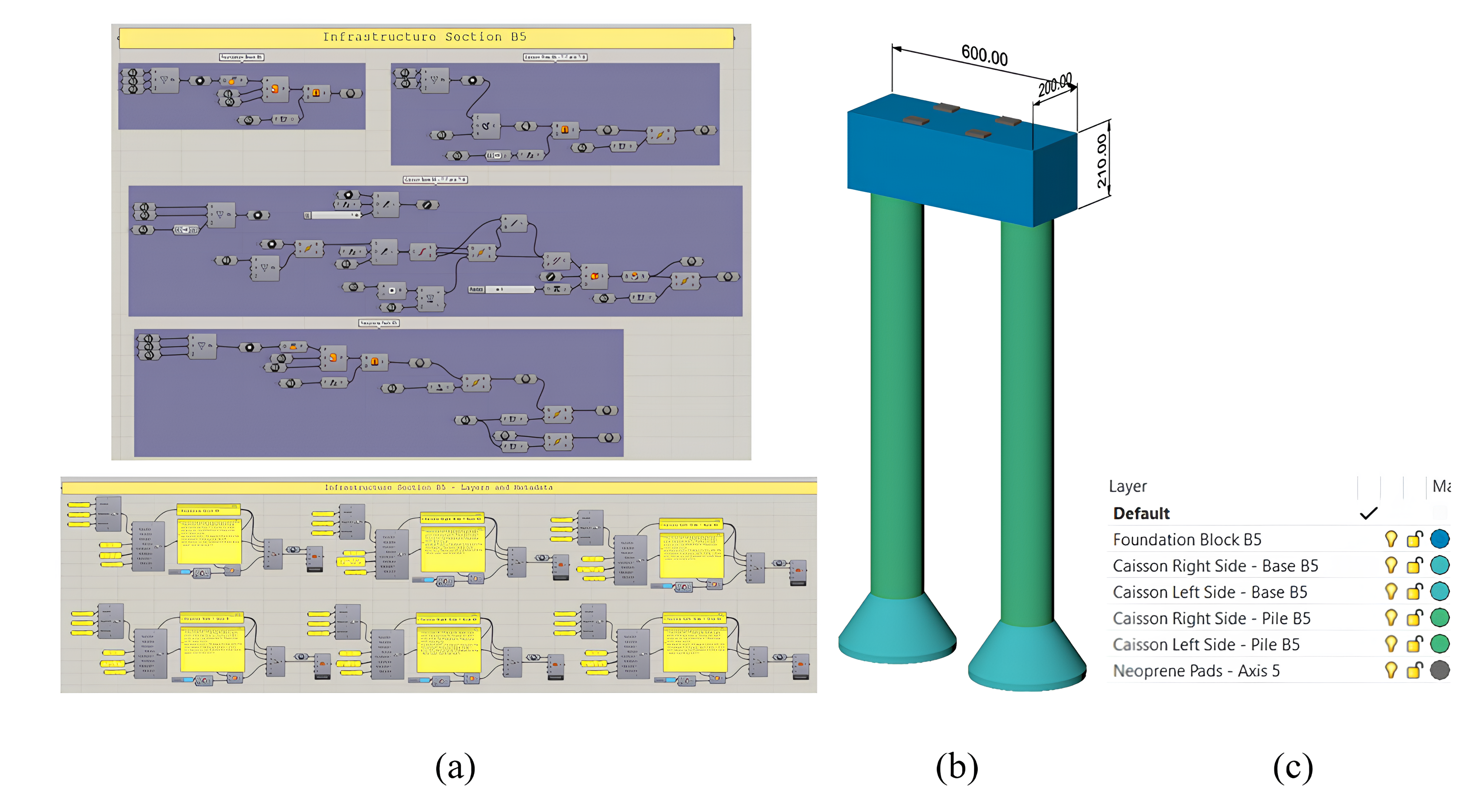
Another advantage of the parameterized model is the possibility of generating geometry in some areas of interest, incorporating metadata in the geometry, and transmitting the information from these regions in layers to pre-processing and analysis software (Figure 1).

Figure 1
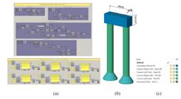
Production of the parameterized model of the railway bridge: (a) part of the code developed in Grasshopper, (b) generated infrastructure elements, dimensions in “cm”, (c) separation of elements into layers.

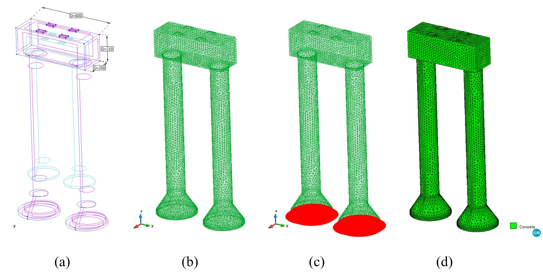
After generating the geometric model, a methodology using the software GiD 15.0.4 [²⁹] was employed for automation and scalability of the pre-processing step. Therefore, programming routines were developed to generate data files to feed different packages of FEM solvers. For this paper, the geometric information generated in the native Rhino “.3dm” format and its metadata were transmitted to the GiD platform, where the implemented routines were employed to generate a data file of the FEM model compatible with the CSiBridge v. 21 [²²] solver. The framework resulted in a model with the unstructured finite element mesh (shell), the support conditions, and materials applied to each region of the analyzed asset, as illustrated in Figure 2. The plugins created for generating pre-process data and migration to the CSiBridge interface contain the following files:

Figure 2
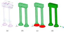
Pre-processing step in GiD: (a) geometry obtained from geometric parameterization (dimensions in “cm”), (b) unstructured finite element mesh with shell elements (12,680 elements, 6,432 nodes and element size of 20 cm), (c) support conditions (fixed support), (d) application of materials.

• Csi_Bridge.bas: responsible for managing and creating the output file called from which all properties launched in the pre-process platform will be migrated to FEM software;

• Csi_Bridge.mat: file containing a list of materials compatible with CSiBridge;

• Csi_Bridge.cnd: file for inserting information about boundary and loading conditions;

• Csi_Bridge.prb: manages the units used in the pre-process model, as well as the type of analysis to be performed according to the finite element selected and the automatic incorporation of the self-weight of the elements that comprise the asset domain.

3 RAILWAY BRIDGE CASE STUDY

Building upon the methodology outlined earlier, this section presents the case study of a reinforced concrete railway bridge in northern Brazil. The study focuses on capturing the bridge structural behavior through a calibrated computational model. The following subsection details the main characteristics of the case study bridge and design considerations.

3.1 Description

Figure 3 illustrates the asset adopted as a case study in this paper. The reinforced concrete railway bridge was built in 1980 and is in the northern region of Brazil, where it is used mainly to transport iron. It has a total length of $180\mathrm{}m$ distributed in two continuous sections: the first includes two 25-meter spans, and the second has four 25-meter spans. Each section ends with abutments, and a five-centimeter expansion was introduced between the two continuous segments at the intermediate support. The bridge superstructure consists of two longitudinal beams with rectangular cross-sections, transverse beams, and a concrete deck with variable cross-sections. The superstructure is supported on the pile caps by neoprene bridge bearings. The infrastructure comprises pile caps supported by caissons and a bedrock layer.

Figure 3
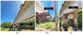
Reinforced concrete railway bridge configuration: (a) general view with detail of the reinforced longitudinal beams, (b) detail of the steel frame reinforcement employed in the bridge rehabilitation process, (c) detail of the bridge expansion joint.

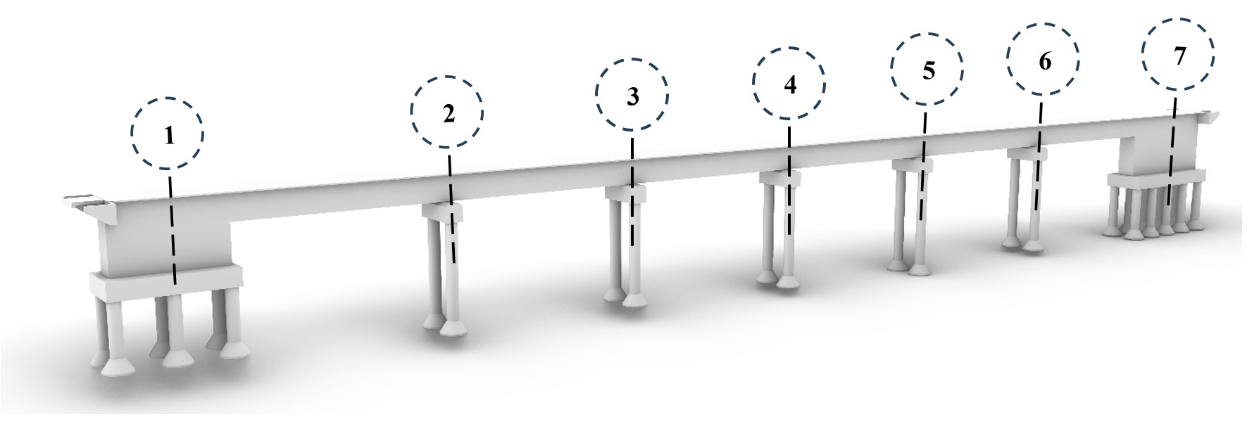
The asset was reinforced in 2017 due to an adverse event. In time, the longitudinal beams were strengthened by increasing their cross-section and the pile cap near one of the abutments. The steel frame adopted during the rehabilitation has remained in use to this day. This element is located close to axis 2 of the asset (Figure 4). The bridge has a hyperstatic configuration, with a $5\mathrm{}cm$ thick expansion joint on axis 3.

Figure 4
Railway bridge geometric model: (a) top view, (b) bottom view, (c) side view with axes, (d) perspective of the railway bridge (dimensions in “cm”).

Figure 4 illustrates the complete geometric model of the bridge. Note the presence of the expansion joint on axis 3, the abutments on axis 1 and 7, the reinforced elements placed during the rehabilitation process in the longitudinal beams between axis 1 and 3, and the bridge pile cap on axis 2.

3.2 Numerical model

Two complementary numerical models of the railway bridge were created, one related to the abutment of axis 1 (Model I), comprising the section between axes 1 and 3 (up to the expansion joint), and the other for the abutment of axis 7 (Model II), comprising the section between axes 3 and 7. This methodology aimed to calibrate each asset region based on vibration modes and natural frequencies obtained during a monitoring campaign carried out in 2020 by a third-party company hired by the asset owner.

The decision to divide the bridge into two numerical models was based on its structural configuration. The asset consists of two continuous segments separated by an expansion joint at intermediate support, allowing each section to behave independently from a structural perspective. This approach ensures that each model accurately reflects the physical behavior of its respective segment while reducing computational demands.

For the materials properties, design data from the railway bridge were used. The shell elements and material properties are found in Table 1. The shell elements’ stiffness parameters had to be calibrated to represent the asset’s dynamic behavior in free vibration. The parameters were defined based on data from the 1980 asset structural design and the strengthening that occurred in 2017. The table provides the following material properties: Young’s modulus $\left(E\right)$, concrete compressive strength $\left(f_c\right)$, and Poisson’s ratio $\left(\right)$. Additionally, the thicknesses of the shell elements $\left(e\right)$ and stiffness coefficients $\left(k_{ij}\right)$, were calibrated according to the 2020 asset instrumentation and monitoring campaign.

Table 1
Material and cross-section properties applied for the computational model.

Bridge region	Material properties	Shell FE properties*
Superstructure (Model I)	E = 24 GPa; ν = 0.2; fc = 18 MPa	Shell thick; e = 25 cm; k12, membrane = 0.65
Infrastructure (Model I)	E = 21.8 GPa; ν = 0.2; fc = 15 MPa	Shell thin; e = 17.5 cm; k12, membrane = 0.80
Strengthening (Model I)	E = 29 GPa; ν = 0.2; fc = 75 MPa	Shell thick; e = 17.5 cm; k12, membrane = 1.00
Superstructure (Model II)	E = 24 GPa; ν = 0.2; fc = 18 MPa	Shell thick; e = 50 cm; k11, membrane = 0.60; k22, membrane = 0.75; k12, membrane = 0.85
Infrastructure (Model II)	E = 21.8 GPa; ν = 0.2; fc = 15 MPa	Shell thin; e = 17.5 cm; k11, membrane = 0.80; k22, membrane = 0.80; k12, membrane = 0.80

• ^*
  1 represents the asset longitudinal direction, 2 the transversal direction, and 3 the vertical direction.

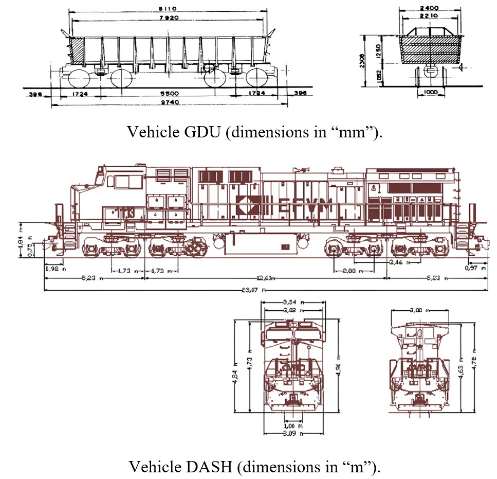
The load configuration for the railway composition consisted of an EVO ES58Aci locomotive, an SD80 locomotive, and a sequence of up to 110 GDU wagons (wagons for transporting iron ore), as shown in Figure 5. This information was provided by the asset owner and represents the railway configuration that was running through the asset at the time of the monitoring stage, the results of which are included in this article. Figure 6 shows a diagram of the loads imposed by the railway composition due to the manufacture of locomotives and GDU wagons. This information is presented for simple verification and may be modified at the manufacturer’s discretion.

Figure 5
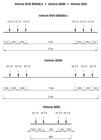
Composition of loads and distances between axles for the vehicle used in dynamic analyses (dimensions in “cm”).

Figure 6
Basic geometric configuration of GDU wagons and locomotives for simple checking.

For the dynamic analysis solution, an area of influence on the railway bridge deck with a width of $1.67\mathrm{}m$ was used, consistent with the width of the tracks. The discretization used was no greater than 1/10 of the lane length. Subsequently, a modal time-history type analysis was used considering the vibration modes and natural frequencies found in the 2020 instrumentation campaign, with damping coefficients of $3.6\mathrm{\%}$ for Model I (experimentally measured), and $1.9\mathrm{\%}$ for Model II, for all vibration modes.

The railway composition speed of $60\mathrm{}km/h$ was used according to data obtained by the asset owner. For time integration, 200 steps were used with a time step every $0.1\mathrm{}s$ and $20\mathrm{}s$ of total analysis time.

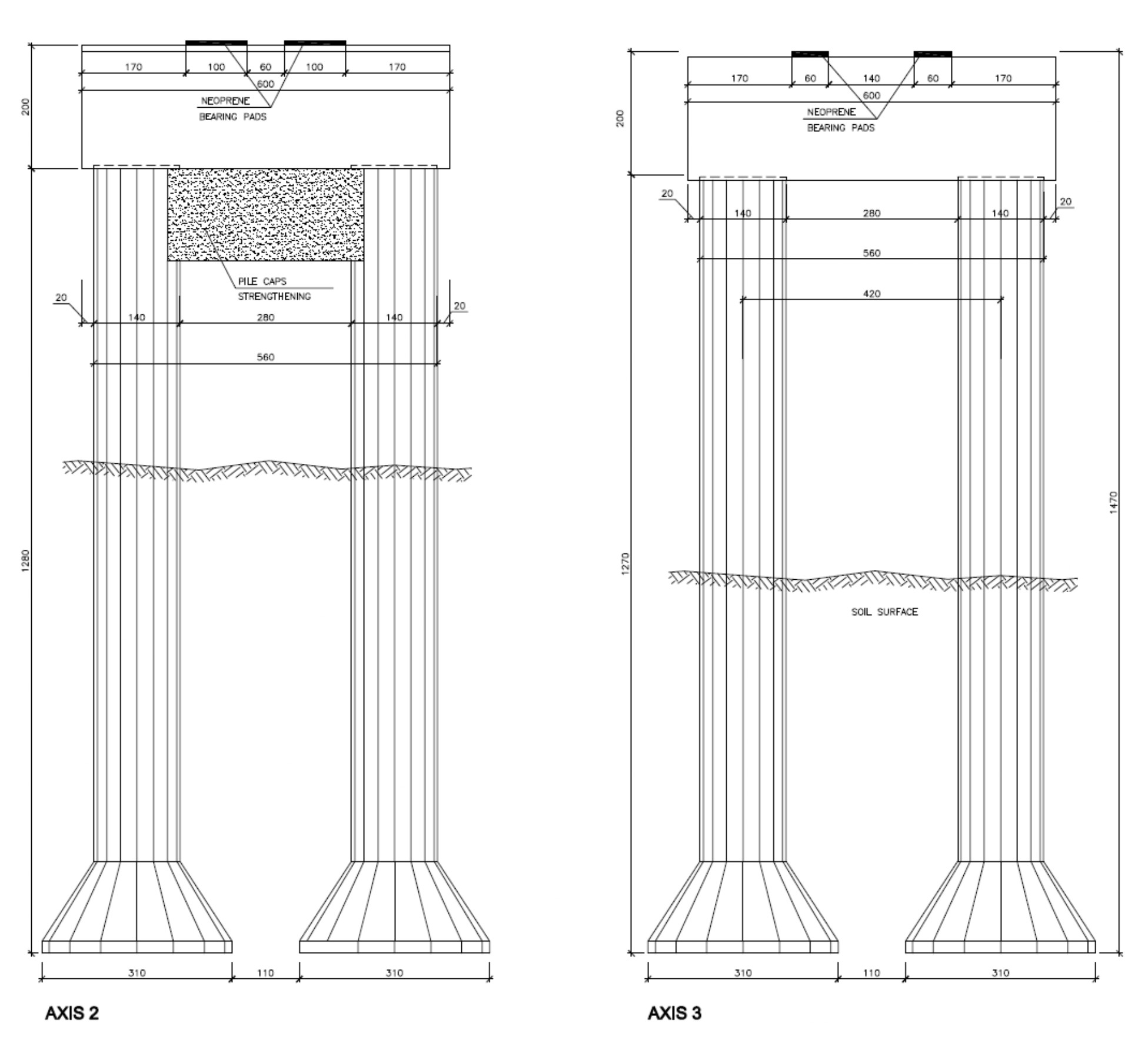
Table 2 and Figure 7 present the construction and stiffness properties used in the support devices on the pile caps according to the SSI model [²⁴] used in this paper and described in Section 2.1.

Table 2
Springs stiffness was adopted for the computational model for Neoprene bearing pads.

Parameters	Asset region
	Axis 2, 4, 5, 6*	Axis 3*
$a\left(m\right)$	0.50	0.35
$b\left(m\right)$	1.00	0.60
${\beta }_3$	137.00	100.00
$k_h=k_1(tf/m)$	7.80	3.30
$k_h=k_2(tf/m)$	-	-
$k_v=k_3(tf/m)$	8131.00	2120.00
$k_{\theta }=k_{{\theta }_1}(tf\bullet m/rad)$	55.70	7.70

• ^*
  Additional properties: $E=2000\mathrm{}MPa;G=1MPa;t=8.0mm;n=8;\mathrm{}{h}_e=64\mathrm{}mm$.

Figure 7
Neoprene bearing pads and pile caps constructive details (dimensions in “cm”).

Figure 8 shows the geometric details of the caissons and pile caps of the asset. Due to the variation in the buried depth of each foundation element, the Winkler spring stiffness values were determined according to the formulation by Morrison [²⁶], as described in Section 2.1.

Figure 8
Constructive details of the railway bridge infrastructure system (dimensions in “cm”).

The spring stiffness values related to the confinement of the caissons were determined based on the methodology proposed by Morrison [²⁶]. Initially, the values were determined for a variation in the foundation depth according to the finite element mesh nodal discretization. The soil characterization test was defined by in-situ testing [²⁷], in which the soil indirect resistance parameter was obtained by the Standard Penetration Test (SPT) [³⁰]. Subsequently, a study was carried out to determine the appropriate number of springs that would simulate the infrastructure soil confinement according to the natural modes and frequencies obtained by the bridge monitoring campaign in 2020.

Springs were not used in the region of the caisson’s widened base due to the highly confined soil conditions and the proximity to the support of the rock foundations. The Winkler spring coefficients for the foundations were therefore determined, as shown in Table 3, using the soil-structure law developed by Morrison [²⁶]. For the landfill regions, spring stiffnesses $k_x=k_y=130\mathrm{}tf/m$ were adopted from the calibration performed using modal analysis.

Table 3
Geotechnical parameters of soil-structure interaction.

Foundation depth (m)	$SPT\left[27\right]$	${\sigma }_{admin}(kN/m^2)$	$k_h(kgf/{cm}^3)$	$k_x=k_y(kN/m)*$
1.0	20.0	392.3	23536	23500
2.0	52	1019.9	81395.2	81340
3.0	63	1235.6	99047.2	98980
4.0	69	1353.3	107873	107800
5.0	72	1412.2	112776.5	112700
6.0	74	1451.4	115718.5	115640
7.0	76	1490.6	119641.1	119560

• ^*
  Additional properties: $S_l=0.70m;D=1.40m.Directions$: X longitudinal, Y transversal, and Z vertical.

The surface soil is mainly formed by sand and the rock by gray phyllite existing in the region supporting the caissons. The water level of the river is approximately at 95.93 m, immediately below the lower region of the pile caps and the river is 4.13 m deep. The elevation at the top of the bridge deck is 101.90 m.

For the steel frame presented in Figure 3, built for the bridge reinforcement stage in 2017, responses from a previous computational model produced by a third-party company, responsible for the bridge instrumentation, were used as input data to obtain the spring stiffness values. Therefore, from a three-dimensional frame numerical model, a distributed load of $100\mathrm{}kN/m$ was applied, obtaining a support reaction equal to $216\mathrm{}kN$ and a vertical displacement of $0.0013\mathrm{}m$. This approach resulted in a vertical Winkler spring stiffness equal to $1700\mathrm{}\mathrm{k}\mathrm{N}/m$. The information fed the bridge dynamic analysis, and the springs were incorporated into the numerical model of this paper to the three support points of the reinforcement steel frame.

4 RESULTS AND DISCUSSION

This section presents and discusses the results obtained from computational models, focusing on validating the methodology and evaluating bridge dynamic performance. Key aspects such as modal analysis, dynamic responses under operational conditions, and structural resilience assessments are explored in detail. The following subsections analyze these outcomes, emphasizing the influence of soil-structure interaction and the implications for railway bridge design and maintenance. These results validate the modeling methodology and provide critical insights into asset performance and resilience.

4.1 Modal analysis

Two computational models related to the abutments of the railway bridge were produced: model I associated with the abutment of axis 1, and model II to the abutment of axis 7, as shown in Figure 9. The properties of the materials used, and the geometry and typology of the shell elements were previously established in Table 1. The natural frequencies and vibration modes were computationally evaluated based on mass participation factors and subsequently compared with the experimental responses obtained by accelerometers and data processing in the ARTEMIS Modal Pro 6.1 software by a third-party company.

Figure 9
Computational models: (a) Model I, axis 1 to 3, 26,230 nodes and 54,869 elements, (b) Model II, axis 3 to 7, 27,801 nodes and 58,815 elements.

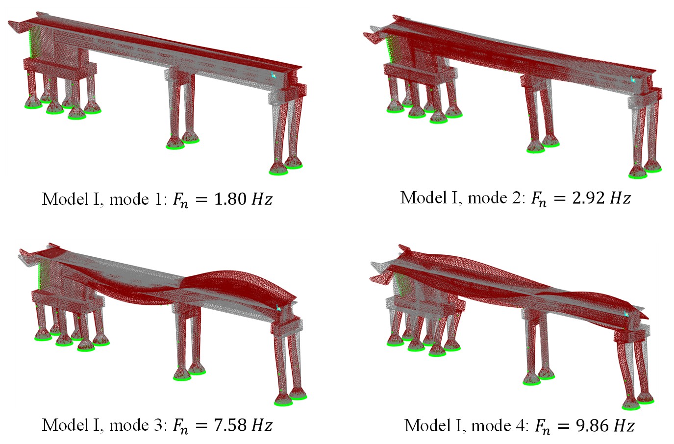
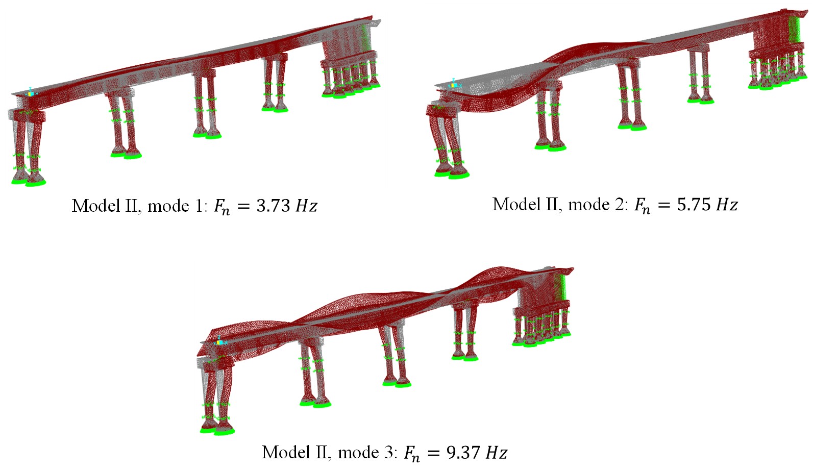
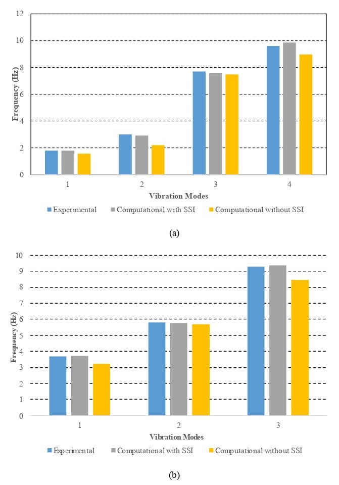
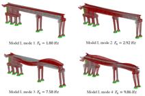
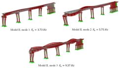
Table 4 presents the modal and mass participation facts obtained for the asset models. The vibration modes and natural frequencies are shown in Figure 10, Figure 11, Figure 12, and Table 5. Models were created by removing springs from the caissons representing the soil in the region of the foundations. It was observed that there was a dispersion of natural frequencies compared to the experimental responses when the soil-structure interaction (SSI) was not considered in the model. The influence of ground confinement is not proportional and depends on the vibration directions of the railway bridge. The computational model considering soil-structure interaction accurately represented the bridge dynamic behavior.

Table 4
Vibration modes and modal participation factors obtained for the railway bridge.

Model	Vibration mode	Period $\left(s\right)$	UX $(kN\bullet cm)$*	UY $(kN\bullet cm)$*	UZ $(kN\bullet cm)$*	$\sum UX$	$\sum UY$	$\sum UZ$
I	In-phase transversal (1)	0.5546	0.0236	3.2255	0.0029	3.1930·10-5	5.9500·10-1	4.7950·10-7
	Antiphase transversal (2)	0.3422	1.0849	1.6141	0.0381	3.8132·10-2	7.4400·10-1	8.3600·10-5
	Longitudinal (3)	0.1319	0.5044	0.1039	0.1342	1.3416·10--1	8.3200·10-1	6.8340·10-3
	Torsional (4)	0.1014	0.0125	0.9122	0.1159	1.1588·10-1	8.8400·10-1	5.7300·10-1
II	Antiphase transversal (1)	0.2682	0.0072	2.0395	0.0107	1.0741·10-2	8.3800·10-1	6.3520·10-4
	Longitudinal (2)	0.1738	0.0441	0.0006	1.7926	8.7900·10--1	8.5500·10-1	6.000·10-2
	Torsional (3)	0.1067	0.0119	0.5695	0.0004	9.1600·10-1	8.7900·10-1	6.7500·10-1

• ^*
  Directions: X longitudinal, Y transversal, and Z vertical.

Figure 10
Frequencies and vibration modes obtained for the models considering SSI: Model I.

Figure 11
Frequencies and vibration modes obtained for the models considering SSI: Model II.

Figure 12
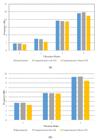
Effect of soil-structure interaction (SSI) in foundations on the natural frequencies of the railway bridge: (a) Model I, (b) Model II.

Table 5
Comparison between natural frequencies and computational and experimental vibration modes.

Model	Vibration mode	Frequency $\left(Hz\right)$			Deviation w/ SSI $\left(\%\right)$	Deviation w/o SSI $\left(\%\right)$
		Computational w/ SSI	Computational w/o SSI	Experimental
I	In-phase transversal (1)	1.80	1.57	1.80	0.00	12.78
	Antiphase transversal (2)	3.00	2.20	2.92	2.74	24.66
	Longitudinal (3)	7.70	7.48	7.58	1.58	1.32
	Torsional (4)	9.60	8.97	9.86	2.64	9.03
II	Antiphase transversal (1)	3.70	3.24	3.73	0.80	13.14
	Longitudinal (2)	5.80	5.68	5.75	0.87	1.22
	Torsional (3)	9.30	8.46	9.37	0.75	9.71

The four probable vibration modes for Model I and three for Model II, identified from mass participation factors, were compared with the experimental results and confirmed from the data obtained during the monitoring stage.

The values presented in Table 4 and Table 5 represent the nodal masses obtained for each mode and natural frequency, with their respective sums and with the mass participation factor depending on the accumulated sum of the masses in each node. The probable vibration modes are verified from the significant increase in the sums of the nodal masses in each global direction and, subsequently, can be confirmed from an instrumentation and monitoring campaign of the asset.

4.2 Dynamic analysis

The calibration of the shell finite elements concerning their stiffness led to representations of the behavior of the railway bridge due to modal analysis, compared to the results from the instrumentation campaign in 2020. Then, after checking the vibration modes and natural frequencies, the dynamic responses of the asset due to railway vehicle passage were verified, as detailed in Section 3.2.

Several dynamic response parameters of the asset were verified, such as accelerations and velocities on the bridge deck, measured with accelerometers, and the dynamic behavior of the pile caps and longitudinal beams, due to displacements and longitudinal strains, measured experimentally, respectively, by displacement transducers (LVDT) and strain gauges. Table 6 presents the results of the dynamic analysis of the asset based on the railway vehicle traffic used on the asset. The shell elements produced excellent precision compared to the experimental results, also in relation to strains on the concrete surface. Previous experiences by the authors had shown that shell finite elements of this order can produce dynamic responses to deformations in pedestrian bridges with composite material decks [⁴].

Table 6
Comparison of computational and experimental results of railway bridge dynamic analysis.

Model	Evaluated parameter*	Computational	Experimental	Deviation.(%)
I	Vertical acceleration on the deck at the midspan between 2 and 3 axes $(m/s²)$	2.30	2.23	3.14
	Vertical velocity on the deck at the midspan between axes 2 and 3 $(mm/s²)$	40.93	48.98	16.44
	Longitudinal acceleration in axis 3 pile caps $(m/s²)$	0.50	0.47	6.38
	Longitudinal velocity in axis 3 pile caps $(mm/s)$	19.35	17.52	10.45
	Vertical displacement in the main girder at axis 3 $\left(mm\right)$	0.70	0.71	1.41
	Longitudinal displacement in the main girder between axes 1 and 2 at midspan $\left(mm\right)$	0.65	0.87	25.29
	Longitudinal strain in the main girder between axes 4 and 5 at midspan $\left(\mu \right)$	80.00	78.00	2.56
II	Vertical velocity on the deck at the midspan between axes 4 and 5 $(mm/s²)$	65.00	60.00	8.33
	Longitudinal velocity in axis 4 pile caps $(mm/s)$	11.07	10.00	10.70
	Longitudinal strain in the main girder between axes 4 and 5 at midspan $\left(\mu \right)$	24.80	22.00	12.73

• ^*
  Notations according to Figure 4.

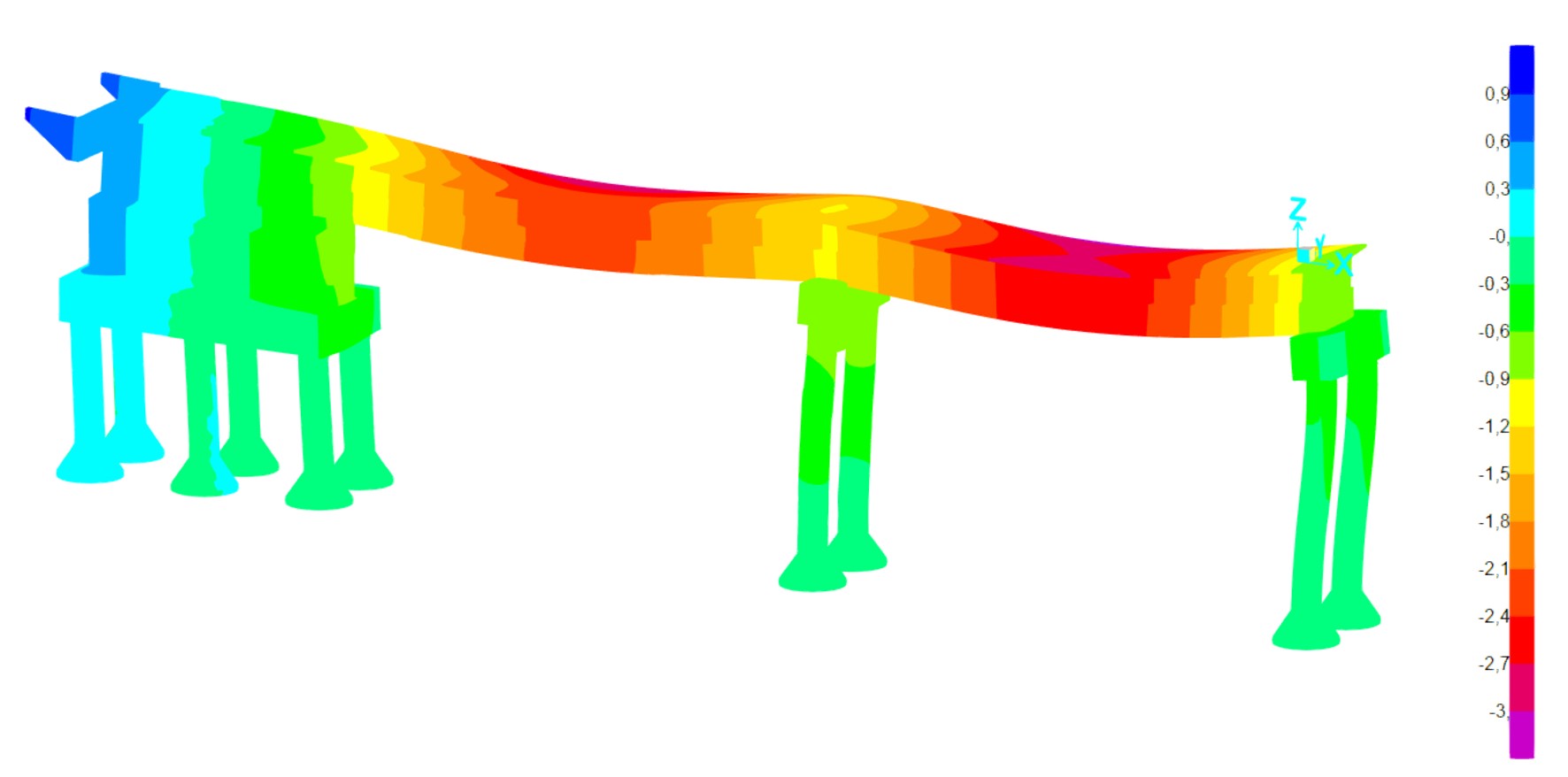
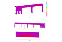
Figure 13 presents the maximum vertical displacements obtained for the dynamic analysis and proposed models. Figure 14 shows the maximum longitudinal deformations for the developed models. Comparing the computational responses to the experimental ones, it was noticed that the regions of maximum deformation were those obtained in the instrumentation campaign, thus validating the technique used in this article.

Figure 13
Maximum vertical displacements for train traffic in “mm” (Model I).

Figure 14
Maximum longitudinal strains for train traffic in “mm”: (a) Model I and (b) Model II.

Regarding the vibration of the asset, there were velocity peaks measured in the computational model and confirmed with monitoring data above $40\mathrm{}mm/s$, which suggests a tendency for the bridge to develop structural problems in the superstructure region [³¹]. For the infrastructure (pile caps), the measured velocities were below $40\mathrm{}mm/s$, suggesting that these elements are intact and without problems regarding excessive vibrations.

4.3 Bridge resilience

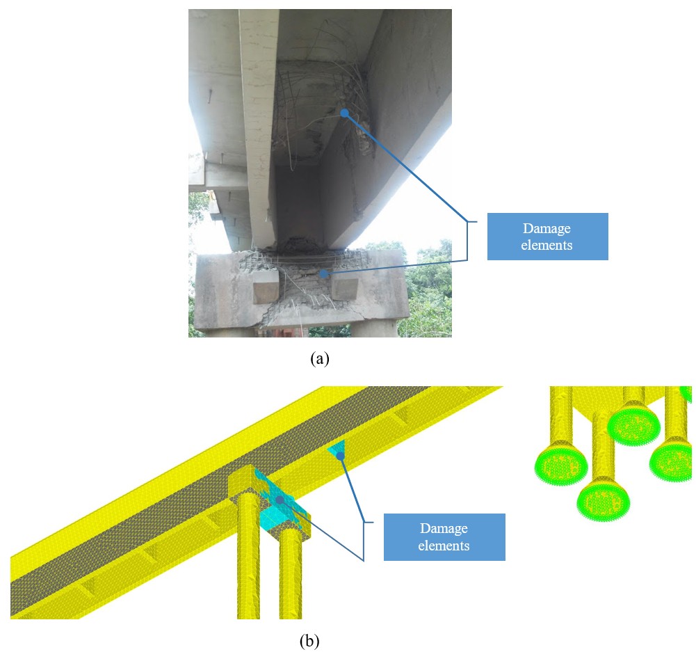
After calibrating the reinforced bridge numerical model (current configuration), a structural resilience study was carried out on the original asset (not strengthened, as shown in Figure 15) due to an external vandalism event that damaged the bridge in 2016. The original asset did not have the strengthening elements and support systems identified in Section 3.1. The damaged region included the pile caps on axis 3 and some transverse beams close to this infrastructure element, as shown in Figure 16.

Figure 15
Railway bridge in original configuration (1980 – 2016).

Figure 16
Quantitative assessment of structural resilience: (a) damage asset and (b) computational strategy.

The computational model was produced (Figure 16) by penalizing the stiffness parameters of the affected elements and maintaining the configuration of the other properties listed in Table 1, except for strengthening elements and the steel frame, which did not exist in the original asset. For the damaged elements, a concrete strength of $0.5\mathrm{}MPa$, Young’s Modulus of $10\mathrm{}MPa$ and shell element thickness of $5\mathrm{}mm$ were used.

The objective of this study was to evaluate the performance of the element for an adverse event based on a computational and quantitative proposal, aiming at the future production of digital twins of the asset [¹⁶] and the verification of its life-cycle [³²] when inducing forced damage.

The methodology used was derived and improved from previous work on the structural resilience of bridges [¹⁹], [²⁰]. In addition to the quantitative approach, the innovation is the use of a computational model calibrated with instrumentation data using shell finite elements and specific laws of soil-structure interaction coupled with the rigidity of the support devices.

Thus, it is possible to determine structural resilience based on localized damage to the asset (superstructure or infrastructure) to compute the severity of the damage induced due to the loss of performance of the railway bridge. The loss of functionality can be represented in different ways, from a reduction in natural frequencies or vibration modes to displacements, accelerations, or velocities calculated from dynamic analyses.

In a previous publication, the authors evaluated the loss of functionality related to longitudinal velocity in the pile caps [²⁰]. The present study is related to the determination of the resilience of the infrastructure system affected by damage due to vertical accelerations in the pile caps.

In general, resilience can be quantified based on an adverse event in the event of loss of functionality of the asset. Thus, the reduction in functionality ${G\left(t\right)}_l$ can be determined from the robustness, calculated by Equation 8:

${G\left(t\right)}_l=1-Z\left(t\right)$ (8)

where $Z\left(t\right)$ represents the robustness of the infrastructure element.

Quantifying resilience depends on the asset’s recovery time from the adverse event, which can be extracted from technical documents or determined considering experience in similar cases. Considering $t$ the time interval for the start of recovery work due to the adverse event and $T$ the time for completion of the repair or reinforcement, we have:

Resilience depends on the asset recovery time due to ${F\left(t\right)}_{loss}$. Thus, using $t_0$ for the start time of the rehabilitation of structural elements and $t_f$ the end time, the angular coefficient of the asset recovery function can be defined with a linear approximation (Equation 9).

$Z\left(t\right)=\frac{{G\left(t\right)}_l}{T-t}$ (9)

where $Z\left(t\right)$ is the rapidity coefficient, considering the loss of functionality and recovery time.

Finally, resilience $Re\left(t\right)$ can be quantified from the area of the resilience triangle, as shown below:

$Re\left(t\right)=1-{0.5\mathrm{}G\left(t\right)}_l\mathrm{}\frac{{G\left(t\right)}_l}{Z\left(t\right)}$ (10)

where $Re\left(t\right)$ represents the quantitative value of resilience, assuming that the relationship between the repair execution time and the recovery of lost performance due to the explosion is linear.

The loss of functionality was determined from the vertical accelerations of the damaged pile cap, present in axis 2 of the bridge, comparing the dynamic responses of the original and damaged asset. The bridge repair and reinforcement activities began on November 11, 2016, and were finished on May 17, 2017.

The resilience parameters were determined according to Equations 8 and 10, thus obtaining the data in Table 7. The resilience and loss of functionality of the asset are found in Figure 17. 187 days were used to reinforce the asset and, based on the resilience data in Table 7, a rapidity of $Z\left(t\right)=0.315\mathrm{\%}/day$ and a resilience of $Re\left(t\right)=45\mathrm{\%}$.

Table 7
Loss of functionality and robustness of the asset.

Computational model	$a_{z,peak}(m/s²)$	${G\left(t\right)}_1\left(\%\right)$	$Z\left(t\right)\left(\%\right)$
Undamaged	0.478	--	--
Damaged	0.760	59.00	41.00

Figure 17
Railway bridge resilience after forced damage: (a) loss of functionality, (b) resilience triangle.

Note that the result of the resilience was impacted by the severe conditions of access to the asset and the mobilization of labor to repair the damage caused in 2016.

In previous work, the authors evaluated the resilience in the railway infrastructure system of the same asset using the loss of functionality related to the longitudinal velocity in the pile caps [²⁰]. The results demonstrated that resilience, determined through longitudinal velocity, was 64%, above the 45% obtained for vertical accelerations. In this way, it was possible to determine the minimum resilience of the railway bridge infrastructure system in the face of the adverse event of an explosion.

Finally, the recovery time of damaged elements directly affects the resilience of the asset according to a non-linear relationship between these variables [²⁰]. However, such determination requires technical documents related to the recovery history of the asset and its parts.

5 CONCLUSIONS

This paper deals with a computational modeling strategy for reinforced concrete railway bridges using dynamic analysis coupled with finite shell elements and soil-structure interaction. Additionally, parameterized geometric modeling and the generation of pre-processing models from implementing programming routines were presented. The computational model was calibrated based on the natural modes and frequencies obtained during an instrumentation campaign of the asset and validated based on the dynamic responses of the railway bridge when the railway train passed. Finally, a structural resilience study was conducted based on an adverse event (explosion) at the asset in 2017.

From the results derived, based on the methodology presented in this work, it can be concluded that:

• The computer modeling technique for reinforced concrete railway bridges using shell elements requires specific parametric calibration studies and depends on results from instrumentation and monitoring campaigns.

• The technique presented demonstrated that the asset’s vibration modes and natural frequencies are sufficient for calibration to compose an engineering solution framework for verifying dynamic analysis data or specific structural resilience studies.

• The modal analysis results showed that using specific soil-structure interaction laws using impedance functions is essential to represent the dynamic behavior of the railway bridge as observed experimentally.

• The development of a parameterized geometric model and pre-processing plugin solutions allow generating a digital twin to feed it with dynamic analysis data originating from a calibrated computational model; like this, the methodology used in this article is promising, as it will feed the development of a digital twin of the asset coupled with life-cycle models.

• The dynamic analysis results pointed to the possibility of structural damage caused to the railway bridge deck due to the velocities determined by the railway traffic.

• The technique for quantitative determination of structural resilience allows creating a datasheet of the asset to seek efficiency in possible rehabilitation work and performance comparisons between different bridges that make up the same railway network.

• It was possible to determine that, for the adverse explosion event that occurred in 2016, the minimum structural resilience value of the foundation block was 45%, determined from the vertical accelerations.

• Another promising product of this paper is the possibility of surveying the dynamic behavior of the asset and its resilience based on damage scenarios induced in the computational model.

• For future developments, we intend to use Abaqus to simulate regions of the asset with submodeling techniques, use the results obtained from the computational model in the digital twin, and apply the methodology described in this article to other assets of interest to the research group.

ACKNOWLEDGEMENTS

This work was financially supported by VALE Catedra Under Rail, FAPESP (grant #2020/02350-2, The São Paulo Research Foundation), and CNPq (The National Council for Scientific and Technological Development, grant #163757/2020-8 and #306379/2021-0).

• Financial support:
  CNPq (grant # 163757/2020-8 and 306379/2021-0), FAPESP (grant # 2020/02350-2).
• Data Availability:
  The data that support the findings of this study are available from the corresponding author, ALG, upon reasonable request.
• How to cite:
  A. L. Gamino, R. R. Santos, T. N. Bittencourt, and M. M. Futai, “Dynamic analysis of railway bridges incorporating soil-structure interaction,” Rev. IBRACON Estrut. Mater., vol. 18, no. 3, e18303, 2025, https://doi.org/10.1590/S1983-41952025000300003

REFERENCES

• ¹ R. R. Santos, H. Carvalho, R. F. Santos, T. N. Bittencourt, and R. B. Caldas, “Comparative study of steel-concrete composite beams for railway bridges,” Rev. IBRACON Estrut. Mater., vol. 17, no. 3, 2024, http://dx.doi.org/10.1590/s1983-41952024000300002.
• ² M. M. Futai et al., “Utilization of digital twins for bridge inspection, monitoring and maintenance,” in Lecture Notes in Civil Engineering, C. Pellegrino, F. Faleschini, M.A. Zanini, J.C. Matos, J.R. Casas and A. Strauss, Eds. 2022, pp. 166–173, https://doi.org/10.1007/978-3-030-91877-4_20.
• ³ A. Z. Kamali, “Dynamic soil-structure interaction analysis of railway bridges: numerical and experimental results,” Licentiate thesis, KTH Roy. Inst. Technol., Stockholm, Sweden, 2018.
• ⁴ A. L. Gamino, M. A. Amaral, R. R. Santos, G. V. Menezes, T. N. Bittencourt, and M. M. Futai, “Soil-structure interaction approach of a timber-concrete composite pedestrian bridge,” Pract. Period. Struct. Des. Constr., vol. 28, no. 3, Aug. 2023, http://dx.doi.org/10.1061/ppscfx.sceng-1261.
• ⁵ K. A. Shaik and G. P. Chandradhara, “Soil structure interaction studies on Krishnaraja Sagara Bridge, Mysuru”, Mater. Today: Proc., vol. 52, no. Part 3, pp. 549–555, 2022, https://doi.org/10.1016/j.matpr.2021.09.496.
• ⁶ A. L. Gamino, R. R. Santos, T. N. Bittencourt, M. M. Futai, and H. Carvalho, “Computational analysis of a reinforced concrete railway bridge considering the soil-structure interaction,” in Life-Cycle of Structures and Infrastructure Systems, F. Biondini and D. M. Frangopol, Eds., London: CRC Press, 2023, pp. 244–251. http://dx.doi.org/10.1201/9781003323020-27.
• ⁷ P. König, P. Salcher, and C. Adam, “An efficient model for the dynamic vehicle-track-bridge-soil interaction system,” Eng. Struct., vol. 253, pp. 113769, Feb. 2022, http://dx.doi.org/10.1016/j.engstruct.2021.113769.
• ⁸ P. Bucinskas and L. V. Andersen, “Dynamic response of vehicle–bridge–soil system using lumped-parameter models for structure–soil interaction,” Comput. Struc., vol. 238, pp. 106270, Oct. 2020, http://dx.doi.org/10.1016/j.compstruc.2020.106270.
• ⁹ Y. Du, Q. Sheng, X. Fu, H. Chen, and G. Li, “New model for predicting the bearing capacity of large strip foundations on soil under combined loading,” Int. J. Geomech., vol. 22, no. 5, May 2022, http://dx.doi.org/10.1061/(asce)gm.1943-5622.0002389.
• ¹⁰ R. Conti and R. Di Laora, “Substructure method revisited for analyzing the dynamic interaction of structures with embedded massive foundations,” J. Geotech. Geoenviron. Eng., vol. 148, no. 6, 2022, https://doi.org/10.1061/(ASCE)GT.1943-5606.0002787.
• ¹¹ A. M. Gharad and R. S. Sonparote, “Evaluation of vertical impact factor coefficients for continuous and integral railway bridges under high-speed moving loads,” Earthq. Eng. Eng. Vib., vol. 20, no. 2, pp. 495–504, Apr. 2021, http://dx.doi.org/10.1007/s11803-021-2034-7.
• ¹² A. A. Faizan and O. Kırtel, “Non-linear soil-structure interaction analysis of railway bridge subjected to earthquake ground motions considering different types of soil”, Arab. J. Geosci., vol. 14, no. 6, pp. 509, Mar. 2021, https://doi.org/10.1007/s12517-021-06834-9.
• ¹³ P. Reumers, G. Lombaert, and G. Degrande, “The effect of foundation–soil–foundation interaction on the response of continuous, multi-span railway bridges,” Eng. Struct., vol. 299, pp. 117096, Jan. 2024, http://dx.doi.org/10.1016/j.engstruct.2023.117096.
• ¹⁴ A. Doménech, M. D. Martínez-Rodrigo, A. Romero, and P. Galvín, “On the basic phenomenon of soil-structure interaction on the free vibration response of beams: application to railway bridges,” Eng. Struct., vol. 125, pp. 254–265, Oct. 2016, http://dx.doi.org/10.1016/j.engstruct.2016.06.052.
• ¹⁵ M. Shamsi and A. Ghanbari, “Seismic retrofit of monorail bridges considering soil–pile–bridge–train interaction,” J. Bridge Eng., vol. 25, no. 10, Oct. 2020, http://dx.doi.org/10.1061/(asce)be.1943-5592.0001613.
• ¹⁶ S. Kaewunruen, M. AbdelHadi, M. Kongpuang, W. Pansuk, and A. M. Remennikov, “Digital twins for managing railway bridge maintenance, resilience, and climate change adaptation,” Sensors, vol. 23, no. 1, pp. 252, Jan. 2023, http://dx.doi.org/10.3390/s23010252.
• ¹⁷ J. N. D. Fernandes, J. C. Matos, H. S. Sousa, and M. R. F. Coelho, “Life cycle analysis of a steel railway bridge over the operational period considering different maintenance scenarios: application to a case study,” Adv. Civ. Eng., vol. 2022, no. 1, Jan. 2022, http://dx.doi.org/10.1155/2022/3010001.
• ¹⁸ P. Bocchini, D. M. Frangopol, T. Ummenhofer, and T. Zinke, “Resilience and sustainability of civil infrastructure: toward a unified approach,” J. Infrastruct. Syst., vol. 20, no. 2, Jun. 2014, http://dx.doi.org/10.1061/(asce)is.1943-555x.0000177.
• ¹⁹ P. Bocchini, D. M. Frangopol, T. Ummenhofer, and T. Zinke, “Resilience and sustainability of civil infrastructure: toward a unified approach,” J. Infrastruct. Syst., vol. 20, no. 2, Jun. 2014, http://dx.doi.org/10.1061/(asce)is.1943-555x.0000177.
• ²⁰ A. L. Gamino, R. R. Santos, T. N. Bittencourt, and M. M. Futai, “Computational analysis of resilience in reinforced concrete railway bridge,” in Bridge Maintenance, Safety, Management, Digitalization and Sustainability, J. S. Jensen, D. M. Frangopol and J. W. Schmidt, Eds., London: CRC Press, 2024, pp. 642–649. https://doi.org/10.1201/9781003483755-74.
• ²¹ G. B. Nica, F. Pavel, and G. Hojda, “A fast nonlinear dynamic analysis automated approach to produce fragility curves for 3D RC frames,” Eng. Struct., vol. 281, pp. 115695, Apr. 2023, http://dx.doi.org/10.1016/j.engstruct.2023.115695.
• ²² CSI. “CsiBridge. 21.” https://www.csiamerica.com/products/csibridge (accessed Oct. 16, 2024).
  » https://www.csiamerica.com/products/csibridge
• ²³ M. S. Silva and F. A. Neves, “Modal identification of Bridge 44 of the Carajás Railroad and numerical modeling using the finite element method,” Rev. IBRACON Estrut. Mater., vol. 13, no. 1, pp. 39–68, Feb. 2020, http://dx.doi.org/10.1590/s1983-41952020000100005.
• ²⁴ L. Guerreiro, A Borracha na Concepção Anti-sísmica. Porto: FEUP, 2003.
• ²⁵ European Committee for Standardization, European standard on structural bearings, CEN/TC 167 WG, 2001.
• ²⁶ N. Morrison, “Interacción suelo-estructuras: semi-espaço de Winkler,” MSc. dissertation, Univ. Politèc. Catalunya – UPC, Barcelona, 1993.
• ²⁷ Associação Brasileira de Normas Técnicas, Soil — Standard Test Method for Standard Penetration Test (SPT) — Test Procedure, ABNT NBR 6884, 2020.
• ²⁸ Robert McNeel & Associates. “Rhino3D. 7.” https://www.rhino3d.com/ (accessed Oct. 16, 2024).
  » https://www.rhino3d.com/
• ²⁹ CIMNE. “GiD Simulation. 15.0.4.” https://www.gidsimulation.com/ (accessed Oct. 16, 2024).
  » https://www.gidsimulation.com/
• ³⁰ D. R. Kumar, P. Samui, A. Burman, W. Wipulanusat, and S. Keawsawasvong, “Liquefaction susceptibility using machine learning based on SPT data,” Intell. Syst. Appl., vol. 20, pp. 200281, Nov. 2023, http://dx.doi.org/10.1016/j.iswa.2023.200281.
• ³¹ German Institute for Standardization, Structural vibration part 3: effects of vibration on structures, DIN 4150-3, 1999.
• ³² J. N. D. Fernandes, J. C. Matos, H. S. Sousa, and M. R. F. Coelho, “Life cycle analysis of a steel railway bridge over the operational period considering different maintenance scenarios: application to a case study,” Adv. Civ. Eng., vol. 2022, 2022, http://dx.doi.org/10.1155/2022/3010001.

Edited by

• Editors:
  Diogo Ribeiro, Daniel Cardoso.

Data availability

The data that support the findings of this study are available from the corresponding author, ALG, upon reasonable request.

Publication Dates

• Publication in this collection
  19 May 2025
• Date of issue
  2025

History

• Received
  16 Oct 2024
• Reviewed
  06 Feb 2025
• Accepted
  15 Mar 2025