Are Port wine export markets integrated? Evidence from price transmission across countries

Os mercados de exportação de vinho do Porto estão integrados? Evidências da transmissão de preços entre países

Abstract

Given the relevance of studies on pricing in international transactions, this paper investigated the extent of market integration among the five most important Port wine export markets, as well as how price changes in one market are transmitted to others globally. This paper analyzed cointegration and price transmission among the five largest export markets for Port wine: Belgium, France, the Netherlands, the United Kingdom, and the United States, based on monthly export data from 1995 to 2017. An ARDL-ECM model is employed to examine price co-movements and market integration using 22 years of data. The results indicated that these markets are not fully integrated, but rather partially integrated. Two main groups emerge: (i) the continental European markets and (ii) the Anglo-Saxon markets. Within each group, markets are reasonably connected. Long-run price transmission is imperfect and nonlinear, while short-run effects are limited, suggesting market segmentation. The France, Netherlands – UK axis shows relatively strong spillover effects. This paper provided an initial contribution to understanding the structure and behavior of Port wine export markets in the global economy, offering insights for both trade strategy and policy formulation.

Keywords:
international trade; ARDL-ECM model; Port wine; market structure; price

Resumo

Dada a relevância dos estudos sobre formação de preços em transações internacionais, este artigo tem como principal objetivo analisar a cointegração e a transmissão de preços entre os cinco maiores mercados de exportação de vinho do Porto: Bélgica, França, Holanda, Reino Unido e Estados Unidos, com base em dados mensais de exportação de 1995 a 2017. Utiliza-se o modelo ARDL-ECM para investigar os comovimentos e a integração de preços no curto e no longo prazo. Os resultados indicam que os mercados não são totalmente integrados, mas sim parcialmente integrados, formando dois grupos principais: os mercados europeus continentais e os anglo-saxões. Dentro de cada grupo, os vínculos são relativamente fortes, com destaque para o eixo França, Holanda, Reino Unido, onde se observam efeitos de transbordamento significativos. A transmissão de preços no longo prazo é imperfeita e não linear; já os efeitos de curto prazo são escassos, sugerindo segmentação de mercado. As conclusões têm implicações para estratégias comerciais e políticas públicas voltadas à promoção das exportações, permitindo que produtores e formuladores de políticas alinhem suas decisões com evidências empíricas sobre o comportamento dos mercados internacionais.

Palavras-chave:
comércio internacional; modelo ARDL-ECM; vinho do Porto; estrutura de mercado; preço

1 Introduction

The internationalization of agri-food markets has increased the complexity of price transmission processes and exposed traditional products to new and varied market dynamics.

Among these, Port wine stands out due to its unique characteristics as a fortified wine with a Protected Designation of Origin (PDO), which confers upon it high symbolic and commercial value. Its production is geographically limited to the Douro Valley in Portugal, and its quality is subjected to strict control by national institutions, making it a relevant case for examining how traditional products behave in international trade.

Despite its prestige and historical relevance, Port wine faces specific challenges in international markets, including competition from other premium wines, variations in consumer preferences, and exchange rate fluctuations. These elements influence both the volume and the pricing of exports. Furthermore, differences in purchasing power and consumption habits across importing countries may lead to segmentation in demand, affecting the strategies of producers and exporters.

Understanding the determinants of price formation and the existence of segmentation patterns is crucial for designing commercial strategies and public policies aimed at enhancing the competitiveness of PDO products. While the literature on price transmission and market integration is vast, there is a gap in empirical studies focusing on the pricing structures of PDO wines in international markets, particularly using methods capable of identifying clusters of countries based on their import behavior.

In the context of wine economics, it is imperative to recognize the uniqueness of this product, not only in terms of its intrinsic complexity but also in terms of its market structure. Wine stands out due to its remarkable price flexibility, reflecting a combination of factors that go beyond simple supply and demand dynamics. Wine is a product of notable complexity, where each variable, from grape variety to vintage weather conditions, contributes to its uniqueness. This complexity is a key factor behind the observed price flexibility in the wine market. Price is influenced by the factors mentioned above as well as by excise taxes, monopoly tariffs, and alcohol taxes (Anderson, 2020).

Among the 4Ps of the marketing mix product, price, place, and promotion (McCarthy, 1960) price is the variable that has the greatest short-term flexibility and can impact the profitability of a business or market (Simon et al., 2008; Kotler & Armstrong, 2015). Wine economics has emerged as a growing field within agricultural economics, but also within other fields such as finance, trade, growth, environmental economics, and industrial organization, as discussed by the authors (Ashenfelter et al., 2018). In this context, price has been a critical factor in helping different actors make purchase decisions (Monroe, 1973, 1990).

In the literature on price (Monroe, 2003; Britannica, 2018; Hung et al., 2021), several studies have been published to date (Graciola et al., 2018; Xia et al., 2021), with emphasis on pricing strategies (Zhen & Xu, 2022), pricing policies (Wu et al., 2022; Sviták et al., 2021), price effects (Sviták et al., 2021), commodity prices (Mohtadi & Castells-Quintana, 2021), intellectual property pricing (Nie et al., 2021), promotional prices (Agrawal & Tang, 2024), value-based pricing (Prieto-Pinto et al., 2020), pricing in electricity markets (Bohland & Schwenen, 2021), pricing distortions (Tan & Wright, 2021), among others (Raja et al., 2020; Schneider & Zielke, 2021).

Muwanga & Snyder (1999) and Baquedano & Liefert (2014) distinguished between partial and perfect market integration, stating that “if trade takes place between spatially separated markets, then prices in one market are related or correlated with the prices in the other markets, in that a price change in one market is partially or totally transmitted to the prices in the other markets in either the short run or the long run.” The perfect transmission of price changes between markets is referred to as perfect or full market integration. Conversely, the lack of integration is referred to as segmentation. A market is geographically segmented if the location of the buyer and seller influences the terms of a transaction in a substantial way, that is, by more than the marginal cost of physically moving the goods from one location to another (Jena, 2016; Gauri et al., 2020; Bassi et al., 2021).

Price transmission in our case refers to spatial price transmission. Fackler & Goodwin (2001), based on Stigler’s (1969) definition of an economic market, argue that when spatially separated markets are considered, price transmission analysis plays a crucial role in assessing how efficiently integrated they are i.e., to what extent rational arbitrage operates (see also Jena, 2016). Other types of price transmission include vertical price transmission, which applies to supply value chains, and cross-commodity price transmission, which denotes the transmission of price changes from one commodity to another.

This paper analyzed cointegration and price transmission among the five largest export markets for Port wine: Belgium, France, the Netherlands, the United Kingdom, and the United States based on monthly export data from 1995 to 2017. This study analyzed the structure of international prices of Port wine, with a specific focus on identifying market segmentation among importing countries. Using descriptive statistics, multivariate techniques, and cluster analysis, we examined whether there are consistent groups of countries that share similar patterns in import prices and volumes. By doing so, we contributed to the literature on international agri-food trade by offering empirical evidence of the existence of segmentation in the global market of a premium PDO product.

In the Brazilian context, studies on agri-food markets focusing on prices and market integration have also been published, as shown in the works of Figueiredo et al. (2017) and Gasques et al. (2020), which reinforces the relevance and timeliness of this study on the international Port wine market.

The paper is organized as follows. In Section 2, we present an overview of recent trends in Port wine exports. Section 3 outlines the data used and the methodology. Section 4 reports the results and provides a discussion. Finally, Section 5 offers the main conclusions of the study.

2 Theoretical Foundation

2.1 Recent trends in Port wine export market: an overview

The wine industry is a specific yet typical example of globalization, displaying a remarkable growth rate in the volume of exports relative to world wine production levels (Anderson & Nelgen, 2011; Pomarici & Vecchio, 2014; Morrison & Rabellotti, 2017; Thome & Paiva, 2020). In 2017, Port wine exports represented 76% of its production, 39% of Portuguese wine exports in value, and 21% in volume. Although, Port wine was exported to 120 countries, the top five importing countries received 73% of Port wine exports (by value) in 2017. France (FR) was the largest importer (24.8%), followed by the United Kingdom (UK), the Netherlands (NL), Belgium (BE), and the United States (US), with shares of 15.6%, 12.4%, 10.1%, and 10.1%, respectively.

To develop this study, the database must be available and reliable, ensuring consistency and comparability with previous studies on the dynamics of wine exports. Furthermore, the structure of the Port wine market has shown stability over time, with the primary destinations maintaining a significant share of exports. In this research, recent data were avoided that may introduce distortions due to exogenous shocks, such as the SARS-COV-2 pandemic crisis, which would undermine the identification of long-term structural patterns.

Port wine has remained a fundamental product of the national economy over the years and represents a symbolic asset of Portugal worldwide. The large variety of grapes allows to produce a diversity of wines, marked by unique characteristics, which enhances their competitiveness in niche markets. Port wine captivates a specific segment of the market, drawn in by both its rich history and its diverse palate. Understanding consumption preferences in different countries is crucial for producers and distributors seeking not only to preserve the tradition of this unique wine but also to adapt their strategies to meet market trends and evolving tastes.

By highlighting the complexity and variety of Port wine from vibrant Rubies (often young, vigorous, and bursting with flavors of red fruits, being less complex and ideal for consumers seeking a more direct and accessible Port wine experience) to sophisticated Tawnies (resulting from extended aging in wooden barrels, giving them an amber color and more complex, evolved flavors) we can better appreciate its unique position in the world of fortified wines (Milheiro et al., 2020).

Appreciation of Port wine varies significantly among different cultures and countries. In the United Kingdom, there is a long tradition of Port wine consumption dating back centuries, when trade treaties between Portugal and England facilitated the importation of this wine. The British have a particular fondness for aged Tawnies and Vintage Ports, enjoying them not only as digestifs but also as part of formal occasions and celebrations. In contrast, other markets may demonstrate distinct preferences, influenced by cultural, gastronomic, and marketing factors. Consumers in emerging or less traditional markets for Port wine may be initially drawn to Rubies due to their accessibility, fruity sweetness, and ease of consumption (Peynaud & Blouin, 1996; Brochado et al., 2021).

These are the key aspects determining why Port wine is competitive and operates in a differentiated market. Prices differ according to production, categories, and consumer preferences, and are transmitted to exports through market differentiation.

The five markets analyzed in this study differ in their preferences for categories of Port wine. For example, FR imports mainly standard Port wine, while the UK and US prefer more expensive categories. British consumers have dominated the Vintage category, where quality and brand prestige are important factors in consumer preferences (Brito, 2006; Hollebeek & Brodie, 2009; Insel, 2014; Dobele et al., 2018).

3 Methodology

In this paper, we examined the price co-movements or price transmission between the five most important Port wine export markets, which represent 73% of the total international trade for this commodity. This network is important for the Portuguese economy, as Port wine exports represent about 40% of the country’s total wine exports.

The data used in this study consist of monthly Port wine exports, in value and quantity, over the period from January 1995 to December 2017, to Belgium (BE), France (FR), the Netherlands (NL), the United Kingdom (UK), and the United States (US). The selected countries represent important consumer markets for Port wine, covering different geographical regions and consumption profiles. By including Belgium, France, the Netherlands, the United Kingdom, and the United States, the study addresses a diversified sample of export destinations.

The data were collected from the COMEXT database, and prices are average prices computed by dividing the total monthly value of exports in euros, by the underlying total quantity, in liters. The period from January 1995 to December 2017 provided a comprehensive view of export trends over more than two decades, allowing for a thorough analysis of price and volume fluctuations over time, as well as the identification of potential long-term patterns. COMEXT is Eurostat's reference database for international trade in goods. It provides access not only to recent and historical data from the European Union (EU) Member States but also to statistics from a significant number of non-EU countries. Although, the euro was introduced in 1999, Eurostat maintains historical data series that are often recalculated or adjusted to ensure compatibility over time. This means that data from 1995 can be analyzed alongside data from later periods, even after the introduction of the euro, allowing for consistent and comparable analyses (Eurostat, 2024; European University Institute, 2024).

The period selected for analysis is from 1995 to 2017, based on the need to capture long-term structural trends in the Port wine export market, enabling the identification of price cycles, seasonality, and patterns of market integration. This timeframe encompasses significant global economic events, such as the Asian financial crisis (1997–1998), the euro crisis, the global recession (2008–2012), and the Brexit referendum (2016), which impacted trade flows and exchange rate dynamics. Additionally, the introduction of the euro in 1999 represented a structural shift in the European economy, reducing exchange rate volatility among eurozone countries and potentially influencing price formation mechanisms in international trade. Beyond macroeconomic factors, wine production is subject to climatic variations, and an extended period allows for the assessment of the impact of extreme weather events on supply and prices.

Finally, the choice of this period is also justified by the availability and consistency of data from the COMEXT database, ensuring comparability over time, even before the euro adoption, and facilitating a robust and statistically coherent analysis. The use of the COMEXT database ensures the reliability and consistency of the data, as it is a recognized and widely used source for international trade information. Calculating monthly average prices by dividing the total export value into euros by the total quantity in liters provides a representative measure of market prices. This approach considers both the financial aspect (export value) and the physical aspect (exported quantity) of commercial transactions. We assume that exchange rates have no impact on prices at the export level.

The assumption that exchange rates have no significant impact on prices at the exporter level can be justified based on the premise that exporters adjust their product prices in response to currency fluctuations, especially in exports to countries with different currencies. Expressing exports in terms of constant prices helps eliminate the effects of inflation over time, allowing for a more accurate analysis of real changes in export values. Moreover, export values are expressed in terms of constant prices.

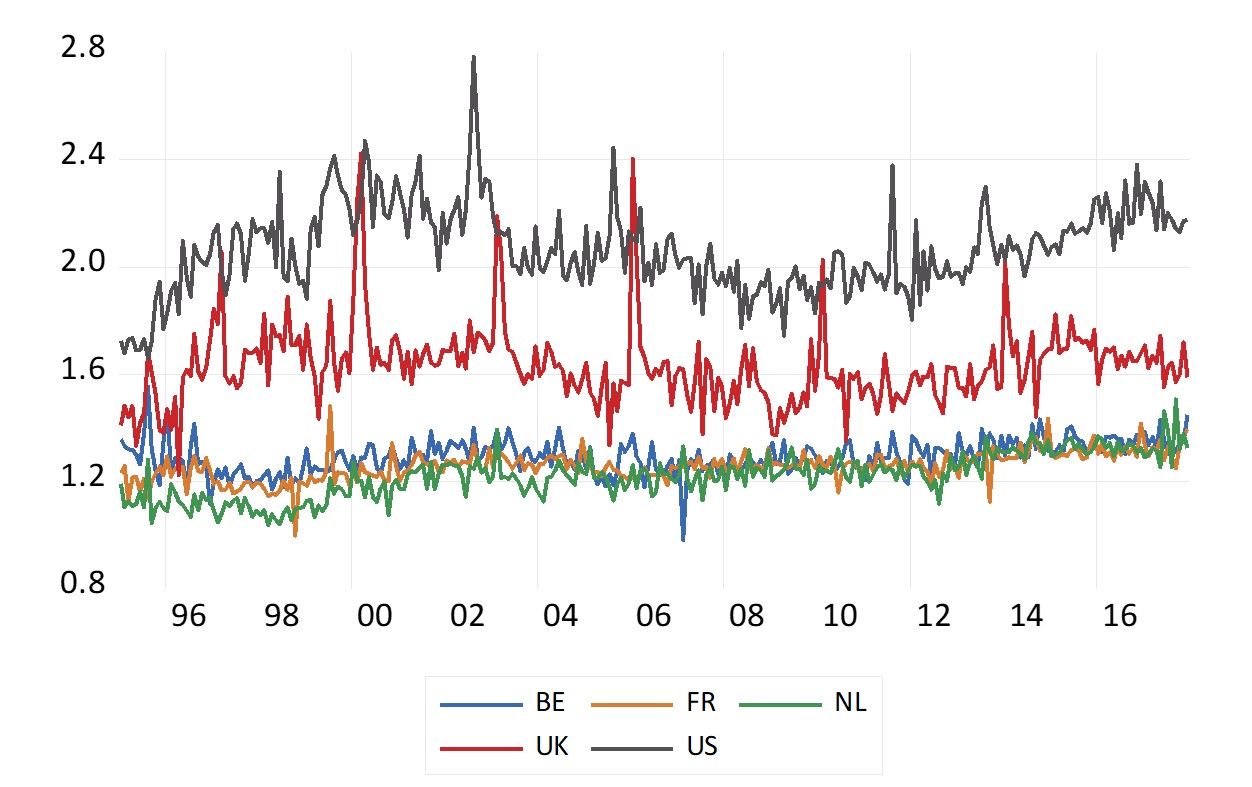
Prices were seasonally adjusted using the multiplicative Census X-12 filter, as the partial correlation function of all price series exhibits peaks of seasonality every 12 months. Finally, we took the natural logarithm of the seasonally adjusted prices to obtain the final series used in our regression models. A chart of these series is displayed in Figure 1.

Figure 1
Seasonally Adjusted Port Wine Log-Prices by Export Market. Notes: Prices are the logarithm of the seasonally adjusted average prices per liter. Higher prices for the UK and the US reflect mainly the difference of quality of exports to these markets, and, in the case of US, the difference in transportation costs, tariffs, etc.

3.1 Long-run market integration

Based on the market definitions mentioned above, one can say that the markets for a group of goods are perfectly integrated if the underlying prices move proportionally to each other over time that is, if the Law of One Price (LOP) holds. The LOP was described by Cassel (1918) over a century ago and can be represented, ceteris paribus, in the basic case of two markets, by a contemporaneous q-power relationship between prices with two parameters:

i) a power parameter q, indicating the degree of nonlinearity in the relationship, and ii) a multiplicative parameter w, which measures the inter-temporal relationship between prices (see Equation 1):

$p_{1t}=w{\left(p_{2t}\right)}^q$ (1)

Thus, the question of this research is: “Are the Port wine export markets horizontally integrated in the sense of Stigler, Sutton, and others, i.e., do Port wine export prices tend to converge to uniformity?” In addition, we are interested in understanding the extent to which price transmission in the Port wine export markets is complete (perfect), incomplete (imperfect), or void (no transmission). Such transmission can be analyzed using a dynamic regression model that identifies separately the short-run and long-run co-movements not explained by pure common stochastic trends. In this case, we can distinguish between instantaneous and long-run horizontal market integration (Slade, 1986; Goodwin et al., 1990; Fackler & Goodwin, 2001; Aguiar-Conraria et al., 2012; Shahzad et al., 2021).

To summarize:

If q ≠ 0, market prices are related or correlated to each other. In this case, there is full or partial price transmission and full or partial market integration.

When q = 1, prices move proportionally, and the LOP holds. In this case, there is full, perfect, or complete price transmission — also known as full or perfect market integration.

When q = 1 and w = 1, the strict version of the LOP holds.

Otherwise, we have the weak version of the LOP when w ≠ 1.

When q < 1, prices move non-proportionally over time and the LOP does not hold.

Finally, when q = 0, there is no price transmission, and markets are said to be segmented.

3.2 ARDL model

The ARDL model studies the co-movements and market integration of Port wine export prices, where some variables are I(0) (stationary), while others are I(1) (nonstationary). The ARDL model was initially proposed by Pesaran & Shin (1999), Baquedano & Liefert (2014), Kalai & Zghidi (2019), and Swei (2020) to build and estimate their preferred Error Correction Model (ECM).

The estimation process comprises two steps. In the first step, we identified the long-run vectors that may exist in the model and estimate the underlying long-run coefficients of the variables. In the second step, we estimate the speed of adjustment to long-run equilibrium, represented by the coefficient of CointEqₜ₋₁, along with the short-run coefficients of the variables.

The general linear model, in the form of an Error Correction Vector (ARDL-ECM) for one dependent variable and k regressors.

When long-run vectors exist in the estimated model, we say that the underlying variables are related in the long run, irrespective of whether they are integrated of order zero or one. Level equations can be estimated to obtain the long-run coefficients of the variables.

To test for the existence of a level relationship in the data, Pesaran et al. (2001), Bentes (2015), and Swei (2020) proposed a Bounds testing approach, wherein the null hypothesis postulates that there is no level relationship. Under the alternative, a long-run relationship does exist, regardless of whether the regressors are purely I(0), purely I(1), or mutually cointegrated.

This test relies on the usual Wald statistic in a generalized Dickey-Fuller-type regression, used to test the significance of lagged levels of the variables under consideration in a conditional Error Correction Regression (Pesaran et al., 2001; Charemza & Deadman, 1997; Dickey & Fuller, 1979). The Wald test statistic is given by Equation 2:

$W_T=\frac{{\left[\widehat{\theta }-{\theta }_0\right]}^2}{1/I_n\left(\widehat{\theta }\right)}$ (2)

where θ denotes the parameter values that maximize the likelihood function (MLE), and I(θ) is the expected Fisher information evaluated at the MLE. The test looks for the difference between the observed and expected information and involves the following steps:

1. Find the MLE

2. Find the expected Fisher information

3. Evaluate the Fisher information at the MLE

From the asymptotic distribution of the Wald statistic, one can obtain the critical values for the two polar cases, I(0) and I(1), which provide critical value bounds for all classifications of the regressors. The Bounds testing procedure is then used as follows: (i) if the value of the F-statistic falls above the critical value bounds, we reject the null of no levels relationship; (ii) if the value of the F-statistic falls below the critical value bounds, we do not reject the null; and (iii) if the value of the F-statistic lies between the bounds, the results are inconclusive.

Note that the conclusions stated in (i) and (ii) can be drawn without needing to know a priori the integration/cointegration status of the underlying regressors (Pesaran et al., 2001; Bentes, 2015; Tsai, 2017; Bontempi et al., 2020). However, if the results are inconclusive, knowledge of the order of integration of the underlying variables is required before conclusive inferences can be made.

Regarding the speed of adjustment to equilibrium, in the second step, the coefficient α of CointEqₜ₋₁ should be negative and statistically significant to denote convergence. Otherwise, a positive coefficient indicates divergence, i.e., a permanent failure to return to equilibrium following a shock to the long-run relationship. The coefficient α shows how much of the disequilibrium is being corrected in each period. If α = 0, there is no adjustment, and claiming a long-run relationship in this case does not make sense (Nkoro & Uko, 2016; Dash, 2019). The short-run coefficients may also be estimated at this step, along with the coefficients of the trend and intercept terms, if they are not included in the level’s equation.

The ARDL model has some advantages relative to conventional cointegration methods, such as the two-step residual-based procedure for testing the null of no cointegration (Engle & Granger, 1987; Kim & Lin, 2018; Churchill et al., 2019), the two-step residual-based procedure for testing the null of cointegration (Shin, 1994; Schild & Schweikert, 2019; Furno, 2020), or the system-based reduced rank regression approach by Johansen (1991); Kim & Lin (2018); Churchill et al. (2019); Furno (2020).

One such advantage is that ARDL can be used regardless of whether the data are stationary I(0), nonstationary I(1), or mutually cointegrated, while conventional methods concentrate on cases in which the underlying variables are I(1). As noted by Cavanagh et al. (1995), this inevitably involves a certain degree of pre-testing for unit roots, thus introducing a further degree of uncertainty into the analysis of levels relationships.

Second, this approach produces better results in capturing long-run relationships for small data samples. Third, regressors’ endogeneity can be fully accounted for when the selected model contains a suitable lag structure, and the residuals are purely white noise. Finally, in the ARDL model, short-run and long-run relationships can be captured simultaneously.

3.3 Model specification

From the general ARDL-ECM model described in Equation 3, we can build our preferred dynamic model, where the optimal number of lags for the dependent variable and the regressors was selected based on the Schwarz Information Criterion (SIC), up to a maximum of 12 lags.

When suitable, to deal with residual heteroskedasticity and autocorrelation, we use the Newey-West (HAC) estimator of the asymptotic covariance matrix with a quadratic-spectral (QS) kernel (Andrews, 1991). The QS kernel has been shown to possess optimality properties in the context of spectral density estimation (Priestley, 1962, 1981) and probability density estimation (Epanechnikov, 1969; Sacks & Ylvisaker, 1981), according to an asymptotic maximum relative MSE criterion and also an asymptotic truncated MSE criterion (Andrews, 1991).

The general linear model, estimated in the form of an Error Correction Vector (ARDL-ECM) for one dependent variable and k regressors, can be specified as follows:

$\text{Δ}{y}_t=\mu +\lambda t+\alpha \left({\beta }_0{y}_{t-1}-{\displaystyle \sum }_{j=1}^k{\beta }_j{x}_{j,t-1}\right)+{\displaystyle \sum }_{i=1}^r{\rho }_i\text{Δ}{y}_{t-i}+{\displaystyle \sum }_{i=0}^{s_j}{\displaystyle \sum }_{j=1}^k{\gamma }_{ji}\text{Δ}{x}_{j,t-i}+{\epsilon }_t$ (3)

where ${\displaystyle \sum }_{i=1}^r{\rho }_i\text{Δ}{y}_{t-i}+{\displaystyle \sum }_{i=0}^{s_j}{\displaystyle \sum }_{j=1}^k{\gamma }_{ji}\text{Δ}{x}_{j,t-i}$ denotes the short-run (SR) term and ${\beta }_0{y}_{t-1}-{\displaystyle \sum }_{j=1}^k{\beta }_j{x}_{j,t-1}$ denotes the long-run (LR) term, which is also known as the cointegration vector or CointEq_t−1. The intercept (μ) and time trend (λt) terms can be added either to the short-run or the long-run equations. As usual, Δ denotes the first difference (or lag) operator, and y and x represent the data variables. Lowercase Greek letters denote parameters to be estimated. The short-run coefficients are represented by ρ and γ; β denotes the long-run coefficients and α denotes the speed of adjustment to equilibrium after a shock or perturbation induced to the long-run equation.

The HAC covariance estimator is only used here when the corresponding pre-ARDL test statistic for heteroskedasticity (Breusch-Pagan-Godfrey) is rejected at the 1\% level. The dynamic linear model is presented in Equations 4 and 5:

$\text{Δ}{Y}_t=\mu +\lambda \text{TREND}+\alpha {\text{CointEq}}_{t-1}+{\rho }_1\text{Δ}{Y}_{t-1}+{\rho }_2\text{Δ}{Y}_{t-2}+{\rho }_3\text{Δ}{Y}_{t-3}+{\gamma }_{10}{\text{ΔX}}_{1t}+{\gamma }_{20}{\text{ΔX}}_{2t}+{\gamma }_{21}{\text{ΔX}}_{\mathrm{2,}t-1}+{\epsilon }_t$ (4)

where

${\text{CointEq}}_{t-1}={\beta }_0{Y}_{t-1}-{\beta }_1{X}_{\mathrm{1,}t-1}-{\beta }_2{X}_{\mathrm{2,}t-1}-{\beta }_3{X}_{\mathrm{3,}t-1}-{\beta }_4{X}_{\mathrm{4,}t-1}-{\beta }_5{X}_{\mathrm{5,}t-1}$ (5)

denotes the long-run (or cointegration) equation and β are the long-run coefficients Carvalho et al. (2020). Note that ${\text{CointEq}}_{t-1}=u_{t-1}$ represents the long-run equation residuals at time t−1. Note also that the regressors X1, …, X5 represent, successively, log export prices for BE, FR, NL, UK and US. When the dependent variable represents a given market, the corresponding X regressor of the underlying equation is dropped. For example, when Y represents the BE market, the X1 regressor also denoting this market is dropped from the equation, and so on. The choice of the ARDL-ECM model for time series analysis is justified by its ability to handle non-stationary series and its effectiveness in identifying long-term relationships and short-term adjustments between variables. While we acknowledge the limitations of time series analysis compared to other methodologies, such as partial equilibrium models, the ARDL-ECM is particularly suitable for capturing price dynamics over time, allowing us to explore not only stationarity and seasonality but also autoregressive effects that are crucial for understanding price dynamics in the wine market.

4 Results and Discussion

4.1 Descriptive statistics

Table 1 presents some basic statistics for the log export prices of Port wine after seasonal adjustment. Descriptive statistics are presented in panel (a). The mean value of the log export prices of Port wine to the UK and the US is about, respectively, 30% and 70% above the corresponding log export prices to continental Europe (BE, FR and NL). The relative dispersion of log prices, given by the coefficient of variation (CV), is also higher for the UK (9%) and the US (8%) than for continental Europe: BE (5%), FR (4%) and NL (7%). Skewness is positive for NL (0.03), UK (1.7) and US (0.4) and negative for BE (−0.2) and FR (−0.1). It is higher in magnitude for the UK and the US than for continental Europe. In addition, for all markets except NL, log export prices exhibit leptokurtosis and drift away from Gaussianity, as shown by the value of the Jarque-Bera statistic. Finally, the unit root (ADF) and trend stationarity (KPSS) test statistics indicate stationarity of all series but the one for BE, where the null of stationarity is rejected in the KPSS test Silva & Amaral (2014);Cunha et al. (2010). These results recommend the use of an ARDL technique to deal with a mixture of I(0)/I(1) variables in our ECM model Table 1.

Table 1
Descriptive Statistics and Pearson Correlation

	BE	FR	NL	UK	US
(a) Descriptive Statístics
Mean	1.293	1.258	1.221	1.629	2.066
Maximum	1.552	1.481	1.506	2.423	2.784
Minimum	0.981	0.999	1.037	1.222	1.659
Std. Dev.	0.063	0.054	0.083	0.147	0.162
CV	4.9%	4.3%	6.8%	9.0%	7.8%
Skewness	-0.165	-0.073	0.026	1.728	0.366
Kurtosis	5.304	5.716	2.858	10.186	4.030
Jarque-Bera	62.310 **	85.097 **	0.263	731.248 **	18.361 **
ADF	-8.188 **	-4.791 **	-5.244 **	-9.252 **	-3.489 **
KPSS	0.180 *	0.116	0.122	0.213	0.197
Obs.	276	276	276	276	276
(b) Pearson Correlation
	BE	FR	NL	UK	US
FR	0.405 **
NL	0.422 **	0.616 **
UK	0.076	0.046	0.081
US	0.089	0.209 **	0.163 **	0.393 **

• Notes: * significant at 5%; ** significant at 1%. Souce: Elaborated by the authors.

Panel (b) of Table 1 presents the Pearson correlation coefficients for the five variables analyzed. All correlations are positive, indicating that price increases in one market tend to be accompanied by increases in others. However, the results show that log export prices in continental European markets (Belgium, France, and the Netherlands) are significantly correlated with each other but not with the UK. The UK, in turn, is positively correlated with U.S. export prices, which are also correlated with France and the Netherlands.

These findings suggested the existence of two relatively distinct export market groups for Port wine: the continental European markets (BE, FR, NL) and the Anglo-Saxon markets (UK, U.S.). The latter group exhibits higher price levels, indicating a pattern of high-quality-oriented consumption. This differentiation can be explained by several factors, such as perceived value—consumers in the UK and U.S. may view Port wine as a luxury or niche product, allowing exporters to charge premium prices.

Additionally, the development of new products based on red and white Port wines has expanded market appeal, especially in gourmet cuisine and tourism, contributing to the growth of exports and international market integration, as highlighted by Ferreira et al. (2020), Milheiro et al. (2020), and Gouveia et al. (2018). Cultural, historical, and income-related factors also play a role in shaping perceptions of value. Moreover, import duties, customs tariffs, and local taxes—often higher in the UK and U.S.—can impact final prices.

Exporters may implement market segmentation strategies, adjusting prices based on demand, competition, and consumer profiles in each country. Logistics and distribution costs can also vary significantly across markets, further influencing final prices. In this context, positioning Port wine as a premium product in select markets allows targeting consumers willing to pay more for quality.

The time series for each group of countries evolves somewhat independently, with strong correlations within each group but limited correlation between them. For example, the UK is only correlated with the U.S., while the U.S. also correlates with France and the Netherlands. This indicated that while some overlap exists, the groups are not perfectly segmented in terms of correlation.

In conclusion, price correlations in the Port wine market among France, the UK, the Netherlands, the U.S., and Belgium result from a combination of economic, cultural, historical, and commercial factors. These interconnected elements shape trade and consumption patterns and influence final prices, which reflect not only production and distribution costs but also the value perceived by consumers.

4.2 Bounds test and long-run form

We have run five ARDL models, one for each Port wine export market as the dependent variable (BE, FR, NL, UK, and US), and used the remaining as dynamic regressors, together with the deterministic regressors. As noted before, the number of lags for each variable in the ARDL model was selected using the Schwarz Information Criterion (SIC). Based on these models, we can test for the existence of a long-run relationship—or level relationship—in the data using the Bounds Test proposed by Pesaran et al. (2001), as well as Bentes (2015) and Swei (2020). A summary of these results is presented in Table 2.

Table 2
ARDL Long Run Form and Bounds Test. Full Model

		BE	FR	NL	UK	US
Regressors		FR, NL, UK, US	BE, NL, UK, US	BE, FR, UK, US	BE, FR, NL, US	BE, FR, NL, UK
Number of specifications evaluated		342,732	342,732	342,732	342,732	342,732
Selected Model		ARDL(1, 0, 0, 0, 0)	ARDL(1, 1, 0, 0, 0)	ARDL(3, 0, 2, 0, 0)	ARDL(1, 0, 1, 0, 0)	ARDL(4, 0, 1, 0, 0)
F-Bounds Test		29.593	45.747	12.499	23.527	5.545
Finite Sample (n=80)	10%	3.644	4.230	4.230	4.230	3.644
Critical Values	5%	4.216	4.840	4.840	4.840	4.216
	1%	5.512	6.164	6.164	6.164	5.512
Breusch-Godfrey Serial	χ2	4.109	3.079	0.471	0.654	1.712
Correlation LM Test	p-value	0.128	0.215	0.790	0.721	0.425
Heteroskedasticity Test:	χ2	6.642	7.452	18.516	11.910	13.623
Breusch-Pagan-Godfrey	p-value	0.249	0.383	0.047	0.104	0.136

• Souce: Elaborated by the authors.

For each model, a total of 342,732 specifications were initially examined by the computer software, and the best one was selected for each dependent variable as follows: BE–ARDL(1, 0, 0, 0, 0), FR–ARDL(1, 1, 0, 0, 0), NL–ARDL(3, 0, 2, 0, 0), UK–ARDL(1, 0, 1, 0, 0), and US–ARDL(4, 0, 1, 0, 0). The symbols represent each export market. The figure in the first position of the numerical sequence represents the number of lags for the dependent variable, followed by the number of lags for each regressor, ordered as they appear in the equation. Thus, for example, for the US, the selected model includes four lags for the dependent variable (US), one lag for the regressor FR, and zero lags for the remaining regressors.

The Bounds Test of Pesaran et al. (2001), Bentes (2015), and Swei (2020) was carried out for each equation, and the corresponding F-statistics were computed. Table 2 presents these results, along with the critical values computed for small finite samples (n = 80) at the 10%, 5%, and 1% levels (see Narayan, 2005). The critical values reported at this stage refer to the case of I(1), since all equations include at least one variable that is likely to be nonstationary (BE). As the critical values for I(1) variables are always higher than those for I(0) variables, we shall not incur misleading inferences when we opt for more “conservative” critical values. For example, in the case of the US (or BE) as the dependent variable, the critical values for I(0) variables in finite samples (n = 80) are, respectively, 2.548 (10%), 3.010 (5%), and 4.096 (1%).

For BE and US, the null hypothesis of no levels relationship is rejected at the 1% level or better if the F-Bounds test statistic is higher than 5.512; the null is not rejected at the 10% level or higher if the F-statistic is less than 3.644; finally, the results are inconclusive if the F-statistic lies between the aforementioned limits. In our case, the results presented in Table 2 show that the null should be rejected at the 1% level both for BE (29.593) and the US (5.545). For the US, however, the result is close to the upper limit of the critical values.

In the case of FR, NL, and UK, the critical value bounds are 4.230 and 6.164. If the value of the statistic lies above the upper bound, we reject the null, and conversely, if it is below the lower bound. Our results showed that for FR (45.747), NL (12.499), and the UK (23.527), we should reject the null of no levels relationship at less than 1%. Therefore, in our case, the Bounds Test of Pesaran et al. (2001), Bentes (2015), and Swei (2020) indicates that long-run (or levels) relationships exist for the five markets analyzed. An ARDL–ECM model can thus be estimated for each market in order to obtain separate coefficients for long-run and short-run shocks. In each equation, the long-run coefficients β are normalized with respect to the dependent variable Y, and each coefficient estimate is given by ${\beta }_j/{\beta }_0$, where j = 1,…, 5.

Table 2 also presents the results of the Breusch–Godfrey Serial Correlation LM Test and the Breusch–Pagan–Godfrey Test of Heteroskedasticity, applied to the residuals of the five ARDL models. In the first case, the null hypothesis of no serial correlation is not rejected at conventional significance levels in any case. With respect to unconditional heteroskedasticity, where HAC covariances were used, the null is marginally rejected at the 5% level for the NL regression. However, an ARCH test (not reported in Table 2) does not reject the null of no conditional heteroskedasticity in any model. The ARDL residuals can, therefore, be said to be i.i.d., although not Gaussian.

Table 3 presents the results of the long-run estimates in the ARDL–ECM regression. In Panel (a), we showed the results for the full models, where all the regressors were used for estimation purposes. In Panel (b), we reported the results for the reduced models, where regressors with non-significant coefficients in the full models were dropped. This fine-tuning of the models led to a substantial increase in the F-Bounds statistic values compared to those obtained for the full models, without altering the stability of the significant coefficients, either in terms of sign, magnitude, or standard error.

Table 3
Long-run Coefficients in the ECM Regression. Levels Equations

	BE			FR			NL			UK			US
(a) Full Model
Variable	Coeff.	S.E.	p-value	Coeff.	S.E.	p-value	Coeff.	S.E.	p-value	Coeff.	S.E.	p-value	Coeff.	S.E.	p-value
BE(t-1)	–	–	–	0.235	0.057	0.000	0.107	0.074	0.149	0.218	0.232	0.348	-0.379	0.518	0.465
FR(t-1)	0.273	0.109	0.013	–	–	–	0.706	0.149	0.000	-0.793	0.431	0.067	2.905	–	0.005
NL(t-1)	0.219	0.071	0.002	0.178	0.056	0.002	–	–	–	0.777	0.289	0.008	–	0.544	0.063
UK(t-1)	0.022	0.034	0.524	-0.012	0.020	0.546	0.085	0.032	0.009	–	–	–	0.539	0.197	0.007
US(t-1)	-0.003	0.032	0.927	0.045	0.018	0.013	-0.013	0.030	0.672	0.346	0.083	0.000	–	–	–
(b) Reduced Model
Variable	Coeff.	S.E.	p-value	Coeff.	S.E.	p-value	Coeff.	S.E.	p-value	Coeff.	S.E.	p-value	Coeff.	S.E.	p-value
BE(t-1)	–	–	–	0.233	0.057	0.000	–	–	–	–	–	–	–	–	–
FR(t-1)	0.271	0.108	0.013	–	–	–	0.757	0.139	0.000	–	–	–	–	–	–
NL(t-1)	0.222	0.070	0.002	0.174	0.056	0.002	–	–	–	0.665	0.268	0.014	0.494	0.217	0.024
UK(t-1)	–	–	–	–	–	–	0.086	0.031	0.005	–	–	–	–	–	–
US(t-1)	–	–	–	0.041	0.017	0.015	–	–	–

• Notes: S.E. denotes the standard error of the estimate. The t-statistic from which the p-value is computed is the ratio Coeff. / S.E. As usual. t−1 denotes the first lag of the variable. Full model includes all variables regardless of the significance level of their coefficient estimates. Reduced model includes only variables with significant coefficient estimates. Souce: Elaborated by the authors.

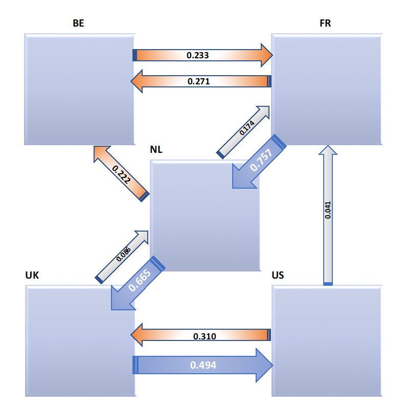
Overall, the long-run results reported in Table 3 indicate that a change in the Port wine export price to BE affects only the export price to FR. In terms of price transmission, this means that an increase of €1 in the export price to BE induces an increase of €0.23 in the export price to FR. Conversely, an increase of €1 in the export price to FR leads to an increase of €0.27 in the export price to BE. A Wald test fails to reject the null hypothesis that these coefficients $$(${\beta }_{12}/{\beta }_{02}{\text{β}}_{12}/{\text{β}}_{02}$a$$ ${\beta }_{21}/{\beta }_{01}{\text{β}}_{21}/{\text{β}}_{01}$)re equal, indicating that price transmission between these markets exhibits a feedback effect of similar magnitude. However, the same €1 increase in the export price of Port wine to FR results in a rise of €0.76 in the export price to NL, while the reverse impact is only €0.17. In this case and others discussed below, Wald tests reject the null of equal coefficients at conventional significance levels. Therefore, a €1 increase in the export price of Port wine to NL leads to a €0.66 increase in the export price to the UK, but the reverse effect is only about €0.09. Finally, the impact of a €1 increase in the Port wine export price to the UK on the export price to the US is €0.49, while the reverse effect is €0.31.

Other effects without reciprocal feedback are also observed. For example, a €1 increase in the export price of Port wine to NL triggers a €0.22 increase in the export price to BE, and a €1 increase in the Port wine export price to the US leads to a €0.04 increase in the export price to FR.

Focusing on the three major market effects mentioned above, we observe that three-quarters of price changes in FR are transmitted to NL, two-thirds of price changes in NL are transmitted to the UK, and half of price changes in the UK are transmitted to the US. In turn, the feedback effect of price changes in the US transmitted back to the UK is about one-third. One-quarter of price changes in FR are transmitted to BE, with a reciprocal effect of similar magnitude, and one-fifth of price changes in NL are transmitted to BE. Some minor long-run feedback effects are also identified in our study. Figure 2 summarizes these findings.

Figure 2
Long-run Coefficients in the ECM Regression. BE = Belgium, FR = France, NL= Netherlands, UK = United Kingdom and US = United States. Arrows denote the direction of the impact. Size of low impact coefficients between 0 and 0.2; size of medium impact coefficients between 0.2 and 0.4; size of high impact coefficients above 0.4. Gray arrow denotes low impact, orange arrow denotes medium impact and blue arrow denotes high impact. All coefficients are significant at the 5% level or better. Source: prepared by the authors

We can; therefore, allocate our long-run results into three main categories: low, medium, and high impact. We arbitrarily define low-impact coefficients as those with a magnitude of up to 0.2. There are three cases in this category: the NL coefficient in the FR regression (0.17), the US coefficient in the FR regression (0.04), and the UK coefficient in the NL regression (0.09).

We define medium-impact coefficients as those between 0.2 and 0.4. There are four such cases: the FR coefficient in the BE regression (0.27), the NL coefficient in the BE regression (0.22), the BE coefficient in the FR regression (0.23), and the US coefficient in the UK regression (0.31).

Finally, we defined high-impact coefficients as those above 0.4. This category includes three cases: the FR coefficient in the NL regression (0.76), the NL coefficient in the UK regression (0.66), and the UK coefficient in the US regression (0.49).

The remaining cases, which are only considered in the full model in Panel (a), can be classified as no-impact coefficients. Although, our network is not fully connected in the long run, there is clear evidence of imperfect or partial market integration in Port wine export prices across the five major markets. The Law of One Price (LOP); however, does not hold in these markets.

4.3 Speed of adjustment to long-run equilibrium

In the second step, we estimated the speed of adjustment to the long-run equilibrium, represented by the coefficient α of CointEqt−1, along with the short-run coefficients of the explanatory variables. We begin this subsection by discussing the speed of adjustment to long-run equilibrium.

Corroborating the results obtained from the Bounds tests and the long-run coefficients presented in the previous subsection, the estimated α coefficients, displayed in Table 4, are all negative and statistically significant at the 1% level or lower, as expected. The estimates retained in the reduced models are virtually identical to those obtained from the full models, reinforcing the finding that the reduced models are adequate for our analytical context.

Table 4
Speed of Adjustment to Long-run Equilibrium in the ECM Regression

	BE			FR			NL			UK			US
(a) Full Model
Variable	Coeff.	S.E.	p-value	Coeff.	S.E.	p-value	Coeff.	S.E.	p-value	Coeff.	S.E.	p-value	Coeff.	S.E.	p-value
CointEq(t-1)	-0.709	0.058	0.000	-0.920	0.060	0.000	-0.646	0.081	0.000	-0.562	0.051	0.000	-0.224	0.042	0.000
Days to recover	42			33			46			53			134
Variable	Coeff.	S.E.	p-value	Coeff.	S.E.	p-value	Coeff.	S.E.	p-value	Coeff.	S.E.	p-value	Coeff.	S.E.	p-value
CointEq(t-1)	-0.707	0.058	0.000	-0.914	0.060	0.000	-0.626	0.080	0.000	-0.560	0.052	0.000	-0.203	0.050	0.000
Days to recover	42			33			48			54			148

• Notes: Full model includes all variables regardless of the significance level of their coefficient estimates. Reduced model includes only variables with significant coefficient estimates. Souce: Elaborated by the authors.

Long-run price shocks occurring in continental European markets are absorbed relatively quickly: approximately 33 days in France (30/0.914), 42 days in Belgium (30/0.707), and 48 days in the Netherlands (30/0.626). Shocks take slightly longer to dissipate in the UK (30/0.560 = 54 days) and significantly longer in the US (30/0.203 ≈ 148 days), where export prices tend to be above average.

Therefore, in terms of speed of adjustment to price shocks, goods and markets may be grouped into continental European and Anglo-Saxon clusters, according to their underlying quality/price relationship. Recall that in these models, α < 0 is required to ensure convergence toward the long-run relationship following a shock to the system.

A long-run relationship is defined by a levels (static) equation, without dynamic regressors, and should not be confused with the duration required to return to equilibrium. In other words, the relevant parameters in the former case are the β coefficients, whereas in the latter case it is the α coefficient.

4.4 Deterministic trends and short-run coefficients

In Table 5, we present the results obtained for the deterministic trends, along with the short-run coefficients of the dynamic regressors. We also included the results for the adjusted R² goodness-of-fit measure. All parameter estimates are statistically significant at the 1% level or lower in the reduced models.

Table 5
Deterministic Trend and Short-run Coefficients

	BE			FR			NL			UK			US
(a) Full Model
Variable	Coeff.	S.E.	p-value	Coeff.	S.E.	p-value	Coeff.	S.E.	p-value	Coeff.	S.E.	p-value	Coeff.	S.E.	p-value
Const.	0.463	0.038	0.000	0.587	0.039	0.000	0.259	0.006	0.005	0.425	0.041	0.000	-0.161	0.032	0.000
@TREND	–	–	–	-1.7E-04	0.000	0.000	3.5E-04	0.000	0.000	–	0.000	0.001	–	–	–
ΔY(t-1)	–	–	–	–	–	–	-0.305	0.073	0.000	-0.393	0.065	0.000	–	–	–
ΔY(t-2)	–	–	–	–	–	–	-0.176	0.057	0.002	-0.218	0.066	0.001	-0.156	0.058	0.008
ΔBEl(t)	–	–	–	0.105	0.036	0.004	–	–	–	0.019	0.136	0.887	0.327	0.130	0.013
ΔFR(t)	–	–	–	–	–	–	0.137	0.059	0.022	–	–	–	–	–	–
ΔFR(t-1)	–	–	–	–	–	–	-0.163	0.060	0.007	–	–	–	–	–	–
Adjusted R2	0.353			0.457			0.483			0.308			0.313
(b) Reduced Model
Variable	Coeff.	S.E.	p-value	Coeff.	S.E.	p-value	Coeff.	S.E.	p-value	Coeff.	S.E.	p-value	Coeff.	S.E.	p-value
Const.	0.481	0.039	0.000	0.579	0.038	0.000	0.034	0.007	0.000	0.154	0.020	0.000	0.259	0.063	0.000
@TREND	–	–	–	-1.7E-04	0.000	0.000	3.4E-04	0.000	0.000	–	0.000	0.000	–	–	–
ΔY(t-1)	–	–	–	–	–	–	-0.319	0.072	0.000	-0.408	0.069	0.000	–	–	–
ΔY(t-2)	–	–	–	–	–	–	-0.183	0.057	0.002	-0.231	0.069	0.001	-0.161	0.060	0.008
ΔBEl(t)	–	–	–	0.104	0.036	0.005	–	–	–	–	–	–	–	–	–
ΔFR(t)	–	–	–	–	–	–	0.149	0.060	0.014	–	–	–	–	–	–
ΔFR(t-1)	–	–	–	–	–	–	-0.168	0.061	0.006	–	–	–	–	–	–
Adjusted R2	0.351			0.456			0.479

• Notes: Full model includes all variables regardless of the significance level of their coefficient estimates. Reduced model includes only variables with significant coefficient. Souce: Elaborated by the authors.

The deterministic constant is positive and significant at less than 1% in all reduced regressions, ranging from 0.03 (NL) to 0.58 (FR). The deterministic time trend is positive and significant at less than 1% in FR and NL, but negative and significant at less than 1% in the UK. These coefficients are small in magnitude, indicating that the series trend very smoothly over the analyzed time.

For example, in the case of FR, prices change at a monthly rate of 0.0002%, and in the case of NL, the monthly rate of price change is approximately 0.0003%. However, time trends are not statistically significant for BE and the US, suggesting that overall price co-movements—both in the long and short run—exert a greater influence on the pricing system than autonomous changes driven solely by the passage of time.

In other words, market integration effects and inter-market linkages outweigh the influence of isolated deterministic trends in explaining price behavior for BE and the US.

With respect to the short-run coefficients of the first-difference dynamic regressors, we found negative autocorrelations for the dependent variable in the NL regression (two lags) and in the US regression (three lags), as well as in the first lagged difference of FR in the NL regression. The autocorrelation estimates decay in magnitude as the lag length increases, indicating that shocks to the system dissipate over time.

Conversely, positive coefficients were found for the first difference of BE in the FR regression and for the first difference of FR in the NL regression. In the latter case, the negative short-run impact that occurs at time t–1 (–0.17) is almost offset by a subsequent positive short-run impact at time t (0.15).

In general, these short-run impacts of BE and FR on the FR and NL regressions, respectively, are small (less than 0.2). However, the autoregressive (memory) short-run effects of the dependent variables NL and US tend to be of low to medium magnitude.

The regressions for BE and the UK; however, do not exhibit statistically significant short-run dynamic coefficients, as shown in Figure 3.

Figure 3
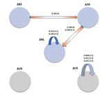
Short-run and autoregressive Coefficients in the ECM Regression. ∆BE = ∆(Belgium), ∆FR = ∆(France), ∆NL = ∆(Netherlands), ∆UK =∆(United Kingdom) and ∆US =∆(United States). Straight arrows denote the direction of the impact. Curved arrows denote autocorrelation effects. Thickness of the arrows denotes the size of the impact. All coefficients are significant at the 5% level or better. Souce: Elaborated by the authors.

We next review the relationship between the dynamic regressors and the dependent variables, measured in first differences, as well as the autoregressive impact, wherever these relationships are relevant. We start with the case of FR, where a positive (negative) variation in BE triggers a positive (negative) change in the variation of FR.

For NL, we identified two types of effects: (i) the autoregressive impact, and (ii) the impact of variations in the dynamic regressor FR on the dependent variable NL, measured in first differences. In the former case, if the auto-variation at time t–1 is larger (smaller) than –0.58 times the auto-variation value at time t–2, then there is a positive (negative) impact on the change in NL from t–1 to t.

In the latter case, if the variation in ΔFR from time t–1 to t is larger (smaller) than 1.13 times the variation in ΔFR from t–2 to t–1, then there is a positive (negative) impact on the change in NL from t–1 to t.

Finally, for the US, we found an autoregressive impact extending up to three lags. The results can be interpreted as follows: if the auto-variation at time t–1 is larger (smaller) than –0.17 times the value at t–2, plus –0.40 times the second-difference value at t–2, then there is a positive (negative) impact on the change in US from t–1 to t.

To conclude, there is weak evidence of short-run co-movements between these markets. Short-run price transmission is observed for BE–FR and FR–NL. Autocorrelation effects are present in NL and the US. But that is all. Market segmentation, therefore, appears to be the most plausible explanation for short-run price co-movements.

The overall fit of the ARDL models highlights, in our case, the advantage of separating short- and long-run effects in Port wine export markets, since the former usually lead to temporary adjustments, while the latter may require structural changes. Furthermore, the results show that short-run impacts are generally of small to medium size, whereas long-run impacts tend to be medium to high, with a strong flow of high transmission between four of the five markets analyzed: FR, NL, UK, and US. These characteristics would not be easily identifiable using only a standard ARDL model, but become evident with the ARDL–ECM specification.

In this study, we analyzed price co-movements among the top five Port wine export markets a network of significant importance for the Portuguese economy. Whether these markets are integrated in terms of price uniformity is a question that may influence firms' pricing and marketing strategies. However, more important than price uniformity at a given moment is the degree to which price changes in one market are transmitted to others over time.

These price transmissions may occur in the short run or long run. The former involves transient adjustments, while the latter may reflect lasting equilibrium dynamics, often implying structural changes. Given their economic relevance, we begin by discussing the long-run impacts of price changes.

The results obtained for long-run relationships clearly indicate the existence of an international export network for Port wine, as strong and significant long-run links connect the five countries analyzed. However, rather than being perfectly integrated in the sense of Stigler (1969) and Sutton (1991), the Port wine export markets appear to be partially integrated and can be divided into two clusters: the continental European markets and the Anglo-Saxon markets.

The interactions among the continental European markets are, in some cases, strong but nonlinear. All coefficients are significantly below one, suggesting that price changes are not fully transmitted between markets. The Anglo-Saxon markets also display strong but nonlinear interactions.

Overall, exporters seem to adjust price/quality strategies to each destination market, as price elasticity varies across countries (Anderson, 2020; Ashenfelter et al., 2018; Viana et al., 2007).

In summary, this analysis highlights the complexity of the Port wine export network, demonstrating how various factors influence price variations and how these fluctuations affect different markets. The identification of two main market groups, and the understanding of their interconnections, provide valuable insights into how exporters tailor their strategies to meet market-specific demands. The lack of consistent short-term linkages suggests that markets may behave independently over short horizons, underscoring the importance of a differentiated approach in export management.

Nevertheless, based on the intensity of price transmission, France appears to lead the continental European group and the UK the Anglo-Saxon group in the long run. The Netherlands seems to serve as the key intermediary market connecting the two groups.

These findings are consistent with the international economics literature, which recognizes that markets are far from perfectly integrated, and that the theories of market segmentation may apply both across and within countries (Engel & Rogers, 1999).

Regarding the short-run links, the scenario is much more limited, and markets are only sporadically interconnected, with some autoregressive effects observed in the cases of the Netherlands and the US. The inclusion of short-run dynamics in the models is; however, essential to avoid biased or inaccurate estimates of long-run relationships.

Based on our results, there is no evidence to support, either strictly or partially, the null hypothesis posed in our research question. Short-run market segmentation thus emerges as the most plausible conclusion, with lower-priced goods predominantly sold in the continental European markets, and higher-priced goods targeting the UK and, especially, the US.

5 Conclusions

The pricing process in the Port wine distribution market encompasses the mechanisms through which producers or exporters set product prices and negotiate terms with distributors or intermediaries. Notably, producers or exporters may exert a degree of market power in this process. This influence stems from various factors, including the perceived quality of Port wine, market demand, supply constraints, and other economic dynamics. As a result, producers or exporters are not merely passive price takers but can actively shape pricing structures within the distribution network.

Market power refers to the ability of a company or group of companies to influence prices or market conditions. In the context of Port wine, producers or exporters may possess market power due to factors such as brand reputation, relative product scarcity, or strong global demand. This may allow them to negotiate more favorable pricing terms with distributors or even impose more advantageous conditions.

The present paper represents a first contribution to the study of the behavior of Port wine export markets in the global economy. In this context, we investigated the degree of market integration among the five most important Port wine export markets. Furthermore, we analyzed how price changes in one market are transmitted to other markets for the same commodity worldwide. To this end, we applied an ARDL–ECM regression model using monthly data over a 22-year period.

Based on the long-run results, we concluded that Port wine export markets are not fully integrated, but rather partially integrated. We identified two main groups: (i) the continental European markets and (ii) the Anglo-Saxon markets. Within each group, markets are reasonably interconnected.

Price transmission is nonlinear in scale and generally associated with small to medium impact coefficients. In other words, price transmission does not occur proportionally across all markets, small price changes in one country do not necessarily lead to proportional changes in others. Impact coefficients, which measure the strength of these effects, tend to be modest. However, the FR–NL–UK axis generates relatively strong spillover effects. In this case, price pass-through is considerable, indicating that price changes in France, the Netherlands, and the United Kingdom have significant cross-border impacts.

Regarding the speed of adjustment to long-run equilibrium after a shock, we find that disturbances dissipate quickly in most cases but take longer to fade in the United States. These shocks refer to abrupt deviations from equilibrium pricing relationships. While most markets revert to equilibrium relatively fast, the adjustment is slower for the US, where export prices are typically higher.

Short-run effects; however, are relatively scarce, reinforcing the case for market segmentation. The results suggest that temporary price variations have limited transmission effects, supporting the notion that markets behave independently in the short term.

These findings have important implications for the determination and negotiation of prices in the Port wine distribution market, where producers or exporters may hold pricing power, either independently or in combination with the market power of importing countries that also produce or export substitute goods—as is the case of France in our sample.

Despite our contribution to the understanding of the structure and functioning of Port wine export markets, several issues remain open for future research. These included, for example, the nonlinear nature of price transmission, the spillover effects of price volatility, and other related dynamics.

Nonetheless, the present study offers a novel and foundational perspective on the global behavior of Port wine export markets, highlighting the interplay between market integration, price dynamics, and international segmentation strategies.

The results also have practical implications for the formulation of commercial strategies within the Portuguese wine sector. Understanding which countries form price-based market segments can help producers and exporters develop targeted marketing strategies, optimize pricing policies, and strengthen negotiations with importers.

Furthermore, these insights may inform public policies related to export promotion and international marketing, particularly in the context of enhancing the global competitiveness of Portuguese Protected Designation of Origin (PDO) wines such as Port. By aligning commercial efforts with empirical evidence on market behavior, stakeholders can more effectively navigate international trade dynamics and reinforce the strategic positioning of the Port wine industry.

The pricing process in the Port wine distribution market encompasses the mechanisms through which producers or exporters set product prices and negotiate terms with distributors or intermediaries. Notably, producers or exporters may exert a degree of market power in this process. This influence arises from factors such as the perceived quality of Port wine, market demand, supply constraints, and broader economic conditions. As a result, they are not merely passive price takers, but actively shape pricing structures within the distribution network.

Market power refers to the ability of a company or group of companies to influence prices or market conditions. In the context of Port wine, a product with Protected Designation of Origin (PDO) status this power may derive from brand reputation, relative scarcity, and sustained international demand, enabling producers to negotiate favorable terms or impose pricing conditions.

This paper presents a first contribution to the understanding of the behavior of Port wine export markets in the global economy. We examined the degree of market integration among the five main export destinations: Belgium, France, the Netherlands, the United Kingdom, and the United States and how price changes in one market are transmitted to others. Using an ARDL–ECM model and monthly export data from 1995 to 2017, we identified two main market clusters: the continental European and the Anglo-Saxon markets. Within each group, price co-movements are stronger, but not complete.

Price transmission is nonlinear and generally modest, though the France, Netherlands–UK axis shows stronger spillover effects. Adjustment to long-run shocks occurs at different speeds, with slower convergence in the United States. Short-run effects are limited, supporting the segmentation hypothesis and suggesting that price dynamics in these markets are partially insulated in the short term.

These findings have practical implications for pricing strategies and negotiations within the distribution chain. Understanding market segmentation patterns allows producers to design pricing policies and commercial strategies that are better aligned with market structures and consumer profiles.

Moreover, this evidence may inform export promotion policies, particularly in reinforcing the global competitiveness of Portuguese PDO wines such as Port. By grounding commercial actions in empirical market analysis, stakeholders can navigate international trade dynamics more effectively.

The incorporation of macroeconomic variables, particularly per capita income, into future analyses represents a relevant perspective to be explored. Investigating whether the absorption of higher-priced Port wines correlates with the income levels of importing countries may enrich the understanding of consumer behavior and market segmentation.

This study contributed to the field of Wine Economics by applying a robust time series approach (ARDL-ECM) to examine price transmission and market segmentation among the main export destinations of Port wine. By identifying two distinct clusters of countries and highlighting asymmetric price relationships, it advances the empirical understanding of market behavior for PDO (Protected Designation of Origin) products in international trade. From a practical perspective, the findings offer insights into public policy aimed at promoting exports, particularly by identifying markets where price strategies can be more effective. Additionally, producers and exporters can use the results to design differentiated pricing and marketing strategies tailored to the specific characteristics and consumer profiles of each market.

Acknowledgements:

CNPq

• How to cite:
  Souza, F. M., Gouveia, S., Ramser, C. A. S., Souza, A. M. & Coronel, D. A., (2026). Are Port wine export markets integrated? Evidence from price transmission across countries. Revista de Economia e Sociologia Rural, 64, e296651. https://doi.org/10.1590/1806-9479.2026.296651
• Financial support:
  CNPq
• Ethics approval:
  Not applicable.
• Data availability:
  The data is available upon request to the authors.
• JEL Classification:
  Q11

6 References

• Carvalho, J. C., Pavan, L. S., & Hasegawa, M. M. (2020). Transmissões de volatilidade de preços entre Commodities agrícolas brasileiras. Revista de Economia e Sociologia Rural, 58(3), e193763. https://doi.org/10.1590/1806-9479.2020.193763
  » https://doi.org/10.1590/1806-9479.2020.193763
• Cunha, D. A. D., Vale, S. M. L. R. D., Braga, M. J., & Campos, A. C. (2010). Integração e transmissão de preços no mercado internacional de café arábica. Revista de Economia e Sociologia Rural, 48(4), 515-542. https://doi.org/10.1590/S0103-20032010000400002
  » https://doi.org/10.1590/S0103-20032010000400002
• Agrawal, S., & Tang, W. (2024). Dynamic pricing and learning with long-term reference effects. arXiv preprint, 72. https://doi.org/10.1145/3670865.3673599
  » https://doi.org/10.1145/3670865.3673599
• Aguiar-Conraria, L., Martins, M. M., & Soares, M. J. (2012). The yield curve and the macro-economy across time and frequencies. Journal of Economic Dynamics & Control, 36(12), 1950-1970. https://doi.org/10.1016/j.jedc.2012.05.008
  » https://doi.org/10.1016/j.jedc.2012.05.008
• Anderson, K., & Nelgen, S. (2011). Wine’s globalization: new opportunities, new challenges. Wine Economics Research Centre Working Paper, (111).
• Anderson, K. (2020). Consumer taxes on alcohol: An international comparison over time. Journal of Wine Economics, 15(1), 42-70. https://doi.org/10.1017/jwe.2020.2
  » https://doi.org/10.1017/jwe.2020.2
• Andrews, D. W. K. (1991). Heteroskedasticity and autocorrelation consistent covariance matrix estimation. Econometrica, 59(3), 817-858. https://doi.org/10.2307/2938229
  » https://doi.org/10.2307/2938229
• Ashenfelter, O., Gergaud, O., Storchmann, K., & Ziemba, W. T. (2018). Handbook of the economics of wine (Vol. 6). Singapure: World Scientific.
• Baquedano, F. G., & Liefert, W. M. (2014). Market integration and price transmission in consumer markets of developing countries. Food Policy, 44, 103-114. https://doi.org/10.1016/j.foodpol.2013.11.001
  » https://doi.org/10.1016/j.foodpol.2013.11.001
• Bassi, F., Pennoni, F., & Rossetto, L. (2021). Market Segmentation and Dynamic Analysis of Sparkling Wine Purchases in Italy. Journal of Wine Economics, 16(3), 283-304. https://doi.org/10.1017/jwe.2021.20
  » https://doi.org/10.1017/jwe.2021.20
• Bentes, S. R. (2015). On the integration of financial markets: How strong is the evidence from five international stock markets? Physica A, 429, 205-214. https://doi.org/10.1016/j.physa.2015.02.070
  » https://doi.org/10.1016/j.physa.2015.02.070
• Bontempi, M. E., Bottazzi, L., & Golinelli, R. (2020). Um índice multinível de dinâmica heterogênea da dívida de curto e longo prazo. Journal of Corporate Finance, 64, 101666. https://doi.org/10.1016/j.jcorpfin.2020.101666
  » https://doi.org/10.1016/j.jcorpfin.2020.101666
• Bohland, M., & Schwenen, S. (2021). Renewable Support and Strategic Pricing in Electricity Markets. International Journal of Industrial Organization, 80, 102792. https://doi.org/10.1016/j.ijindorg.2021.102792
  » https://doi.org/10.1016/j.ijindorg.2021.102792
• Britannica. (2018). Price encyclopedia Britannica Chicago: The Britannica Group.
• Brito, C. (2006). A network perspective of the port wine sector. International Journal of Wine Marketing, 18(2), 124-138. https://doi.org/10.1108/09547540610681103
  » https://doi.org/10.1108/09547540610681103
• Brochado, A., Stoleriu, O., & Lupu, C. (2021). Wine tourism: a multisensory experience. Current Issues in Tourism, 24(5), 597-615. https://doi.org/10.1080/13683500.2019.1649373
  » https://doi.org/10.1080/13683500.2019.1649373
• Cassel, G. (1918). Abnormal deviations in international exchanges. Economic Journal (London), 28(112), 413-415. https://doi.org/10.2307/2223329
  » https://doi.org/10.2307/2223329
• Cavanagh, C. L., Elliott, G., & Stock, J. H. (1995). Inference in models with nearly integrated regressors. Econometric Theory, 11(5), 1131-1147. https://doi.org/10.1017/S0266466600009981
  » https://doi.org/10.1017/S0266466600009981
• Charemza, W., & Deadman, D. 1997. New directions in econometric practice general to specific modelling, cointegration and vector autoregression (2nd ed.). Cheltenham: Edward Elgar Publishing.
• Ferreira, C., Rebelo, J., Lourenço-Gomes, L., Correia, E., Baumert, P., & Plumejeaud-Perreau, C. (2020). Consumer preferences and purchasing rationales for wine: a multivariate data analysis. New Medit, 19(4), https://doi.org/10.30682/nm2004i
  » https://doi.org/10.30682/nm2004i
• Churchill, S. A., Inekwe, J., Ivanovski, K., & Smyth, R. (2019). Dynamics of oil price, precious metal prices and the exchange rate in the long-run. Energy Economics, 84, 104508. https://doi.org/10.1016/j.eneco.2019.104508
  » https://doi.org/10.1016/j.eneco.2019.104508
• Dash, S. K. (2019). Has the Feldstein-Horioka puzzle waned? Evidence from time series and dynamic panel data analysis. Economic Modelling, 83, 256-269. https://doi.org/10.1016/j.econmod.2019.02.015
  » https://doi.org/10.1016/j.econmod.2019.02.015
• Dickey, D. A., & Fuller, W. A. (1979). Distribution of the estimators for autoregressive time series with a unit root. Journal of the American Statistical Association, 74, 427-431. https://doi.org/10.2307/228634
  » https://doi.org/10.2307/228634
• Dobele, A. R., Greenacre, L., & Fry, J. (2018). The impact of purchase goal on wine purchase decisions. International Journal of Wine Business Research, 30(1), 19-41. https://doi.org/10.1108/IJWBR-07-2016-0021
  » https://doi.org/10.1108/IJWBR-07-2016-0021
• Eurostat. (2024). Information on data Retrieved in 2024, March 25, from https://ec.europa.eu/eurostat/web/international-trade-in-goods/data
  » https://ec.europa.eu/eurostat/web/international-trade-in-goods/data
• European University Institute. (2024). Eurostat: official EU statistical data Retrieved in 2024, March 25, from https://www.eui.eu/Research/Library/ResearchGuides/Economics/Statistics/DataPortal/EDD
  » https://www.eui.eu/Research/Library/ResearchGuides/Economics/Statistics/DataPortal/EDD
• Engel, C., & Rogers, J. H. (1999). Violating the law of one price: should we make a federal case out of it? (NBER Working Paper Series, No. 7242). Cambridge: National Bureau of Economic Research.
• Engle, R. F., & Granger, C. W. J. (1987). Cointegration and error correction representation: estimation and testing. Econometrica, 55(2), 251-276. https://doi.org/10.2307/1913236
  » https://doi.org/10.2307/1913236
• Epanechnikov, V. A. (1969). Non-parametric estimation of a multivariate probability density. Theory of Probability and Its Applications, 14(1), 153-158. https://doi.org/10.1137/1114019
  » https://doi.org/10.1137/1114019
• Fackler, P. L., & Goodwin, B. K. (2001). Spatial price analysis. In B. L. Gardner, & C. G. Rausser (Eds.), Handbook of agricultural economics (Vol. 1, pp. 971-1024). San Diego: Elsevier Science & Technology. https://doi.org/10.1016/S1574-0072(01)10025-3
  » https://doi.org/10.1016/S1574-0072(01)10025-3
• Figueiredo, A. M., Braga, M. J., & Teixeira, E. C. (2017). Price transmission in the Brazilian soybean market: an analysis based on cointegration models. Revista de Economia e Sociologia Rural, 55(1), 123-140. https://doi.org/10.1590/1234-56781806-94790550108
  » https://doi.org/10.1590/1234-56781806-94790550108
• Gasques, J. G., Bastos, E. T., & Bacchi, M. R. P. (2020). Competitividade da agricultura brasileira: análise da evolução recente. Revista de Economia e Sociologia Rural, 58(1), 1-18. http://doi.org/10.1590/1806-9479.2020.186209
  » http://doi.org/10.1590/1806-9479.2020.186209
• Furno, M. (2020). Cointegration tests at the quantiles. International Journal of Finance & Economics, 26(1), 1087-1100. https://doi.org/10.1002/ijfe.1837
  » https://doi.org/10.1002/ijfe.1837
• Gauri, D. K., Jindal, R. P., Ratchford, B., Fox, E., Bhatnagar, A., Pandey, A., & Howerton, E. (2020). Evolution of retail formats: Past, present, and future. Journal of Retailing, 97(1), 42-61. https://doi.org/10.1016/j.jretai.2020.11.002
  » https://doi.org/10.1016/j.jretai.2020.11.002
• Goodwin, B. K., Grennes, T. J., & Wohlgenant, M. K. (1990). Testing the law of one price when trade takes time. Journal of International Money and Finance, 5(1), 682-693. https://doi.org/10.1016/0261-5606(90)90003-I
  » https://doi.org/10.1016/0261-5606(90)90003-I
• Graciola, A. P., De Toni, D., Lima, V. Z., & Milan, G. S. (2018). Does price sensitivity and price level influence store price image and repurchase intention in retail markets? Journal of Retailing and Consumer Services, 44, 201-213. https://doi.org/10.1016/j.jretconser.2018.06.014
  » https://doi.org/10.1016/j.jretconser.2018.06.014
• Hollebeek, L. D., & Brodie, R. J. (2009). Wine service marketing, value co‐creation and involvement: research issues. International Journal of Wine Business Research, 21(4), 339-353. https://doi.org/10.1108/17511060911004914
  » https://doi.org/10.1108/17511060911004914
• Hung, H.-H., Cheng, Y.-H., Chuang, S.-C., Yu, A. P.-I., & Lin, Y.-T. (2021). Consistent price endings increase consumers perceptions of cheapness. Journal of Retailing and Consumer Services, 61, 102590. https://doi.org/10.1016/j.jretconser.2021.102590
  » https://doi.org/10.1016/j.jretconser.2021.102590
• Insel, B. (2014). The evolving global wine market. Business Economics (Cleveland, Ohio), 49(1), 46-58. https://doi.org/10.1057/be.2014.3
  » https://doi.org/10.1057/be.2014.3
• Jena, P. K. (2016). Commodity market integration and price transmission: empirical evidence from India. Theoretical and Applied Economics, vol. XXIII, 3(608), 283-306.
• Johansen, S. (1991). Estimation and hypothesis testing of cointegrating vectors in Gaussian vector autoregressive models. Econometrica, 59(6), 1551-1580. https://doi.org/10.2307/2938278
  » https://doi.org/10.2307/2938278
• Kalai, M., & Zghidi, N. (2019). Foreign direct investment, trade, and economic growth in MENA countries: empirical analysis using ARDL bounds testing approach. Journal of the Knowledge Economy, 10(1), 397-421. https://doi.org/10.1007/s13132-017-0460-6
  » https://doi.org/10.1007/s13132-017-0460-6
• Kim, D. H., & Lin, S. C. (2018). The resource curse hypothesis: Dynamic heterogeneous approach. Emerging Markets Finance & Trade, 54(12), 2698-2717. https://doi.org/10.1080/1540496X.2017.1372281
  » https://doi.org/10.1080/1540496X.2017.1372281
• Kotler, P., & Armstrong, G. (2015). Princípios de marketing (15th ed.). São Paulo: Pearson Education do Brasil.
• Xia, Y., Xie, J., Zhu, W., & Liang, L. (2021). Pricing strategy in the product and service market. Journal of Management Science and Engineering, 6(2), 211-234. https://doi.org/10.1016/j.jmse.2021.02.001
  » https://doi.org/10.1016/j.jmse.2021.02.001
• Milheiro, J., Cosme, F., Filipe-Ribeiro, L., & Nunes, F. M. (2020). Port Wine: Production and Ageing. In F. Cosme (Ed.), Chemistry and biochemistry of winemaking, wine stabilization and aging London: IntechOpen.
• Mccarthy, J. (1960). Basic marketing: a managerial approach Chicago: lrwin.
• Mohtadi, S., & Castells-Quintana, D. (2021). The distributional dimension of the resource curse: Commodity price shocks and income inequality. Structural Change and Economic Dynamics, 59, 63-78. https://doi.org/10.1016/j.strueco.2021.08.002
  » https://doi.org/10.1016/j.strueco.2021.08.002
• Monroe, K. B. (1973). Buyers’ subjective perceptions of price. JMR, Journal of Marketing Research, 10(1), 70-80.
• Monroe, K. B. (2003). Princing making profitable decisions (3rd ed.). New York: McGraw-Hill.
• Monroe, K. B. (1990). Pricing: making profitable decision New York: McGraw-Hill.
• Muwanga, G. S., & Snyder, D. L. (1999). Market integration and the law of one price: an empirical comparison of alternative estimation approaches (Economic Research Institute Study Paper, No. ERI#99-22). Logan: Utah State University. Retrieved in 2024, March 25, from https://digitalcommons.usu.edu/eri/172
  » https://digitalcommons.usu.edu/eri/172
• Narayan, P. K. (2005). The saving and investment nexus for China: evidence from cointegration tests. Applied Economics, 37(17), 1979-1990. https://doi.org/10.1080/00036840500278103
  » https://doi.org/10.1080/00036840500278103
• Nie, P. Y., Chen, Z. R., & Wang, C. (2021). Intellectual property pricing under asymmetric duopoly. Journal of Retailing and Consumer Services, 58, 102261. https://doi.org/10.1016/j.jretconser.2020.102261
  » https://doi.org/10.1016/j.jretconser.2020.102261
• Nkoro, E., & Uko, A. K. (2016). Autoregressive distributed lag (ARDL) cointegration technique: application and interpretation. Journal of Statistical and Econometric Methods, 5(4), 63-91.
• Pesaran, M. H., & Shin, Y. (1999). An autoregressive distributed lag modelling approach to cointegration analysis. In S. Strom, (Ed.), Econometrics and economic theory in the 20th century: the ragnar frisch centennial symposium (pp. 371-413). Cambridge: Cambridge University Press. https://doi.org/10.1017/CCOL521633230.011
  » https://doi.org/10.1017/CCOL521633230.011
• Pesaran, M. H., Shin, Y., & Smith, R. J. (2001). Bounds testing approaches to the analysis of level relationships. Journal of Applied Econometrics, 16(3), 289-326. https://doi.org/10.1002/jae.616
  » https://doi.org/10.1002/jae.616
• Peynaud, E., & Blouin, J. (1996). The taste of wine: the art science of wine appreciation Hoboken: John Wiley & Sons.
• Pomarici, E., & Vecchio, R. (2014). Millennial generation attitudes to sustainable wine: An exploratory study on Italian consumers. Journal of Cleaner Production, 66, 537-545. https://doi.org/10.1016/j.jclepro.2013.10.058
  » https://doi.org/10.1016/j.jclepro.2013.10.058
• Priestley, M. B. (1962). Basic considerations in the estimation of spectra. Technometrics, 4(4), 551-564. https://doi.org/10.1080/00401706.1962.10490039
  » https://doi.org/10.1080/00401706.1962.10490039
• Priestley, M. B. (1981). Spectral analysis and time series (Vol. I-II). New York: Academic Press.
• Prieto-Pinto, L., Garzón-Orjuela, N., Lasalvia, P., Castañeda-Cardona, C. D. R., & Rosselli, D. (2020). International experience in therapeutic value and value-based pricing: a rapid review of the literature. Value in Health Regional Issues, 23, 37-48. https://doi.org/10.1016/j.vhri.2019.11.008
  » https://doi.org/10.1016/j.vhri.2019.11.008
• Raja, J. Z., Frandsen, T., Kowalkowski, C., & Jarmatz, M. (2020). Learning to discover value: value-based pricing and selling capabilities for services and solutions. Journal of Business Research, 114, 142-159. https://doi.org/10.1016/j.jbusres.2020.03.026
  » https://doi.org/10.1016/j.jbusres.2020.03.026
• Sacks, J., & Ylvisaker, D. (1981). Asymptotically optimum kernels for density estimation at a point. Annals of Statistics, 9(2), 334-346. https://doi.org/10.1214/aos/1176345399
  » https://doi.org/10.1214/aos/1176345399
• Schild, K. H., & Schweikert, K. (2019). On the validity of tests for asymmetry in residual-based threshold cointegration models. Ekonometria, 7(1), 12. https://doi.org/10.3390/econometrics7010012
  » https://doi.org/10.3390/econometrics7010012
• Schneider, P. J., & Zielke, S. (2021). Price versus service: can retailers beat showrooming with competence? Journal of Retailing and Consumer Services, 61, 102592. https://doi.org/10.1016/j.jretconser.2021.102592
  » https://doi.org/10.1016/j.jretconser.2021.102592
• Shahzad, S. J. H., Arreola‐Hernandez, J., Rahman, M. L., Uddin, G. S., & Yahya, M. (2021). Asymmetric interdependence between currency markets’ volatilities across frequencies and time scales. International Journal of Finance & Economics, 26(2), 2436-2457. https://doi.org/10.1002/ijfe.1915
  » https://doi.org/10.1002/ijfe.1915
• Shin, Y. (1994). A residual-based test of the null of cointegration against the alternative of no cointegration. Econometric Theory, 10(1), 91-115. https://doi.org/10.1017/S0266466600008240
  » https://doi.org/10.1017/S0266466600008240
• Silva, A. L., & Amaral, T. P. (2014). Integração entre mercados regionais de arroz no Brasil: uma aplicação do modelo VEC. Revista de Economia e Sociologia Rural, 52(2), 327-344.
• Simon, H., Bilstein, F. R., & Luby, F. (2008). Gerenciar para o lucro, não para a participacão de mercado Porto Alegre: The Bookman.
• Slade, M. E. (1986). Exogeneity test of market boundaries applied to petroleum products. The Journal of Industrial Economics, 34(3), 291-304. https://doi.org/10.2307/2098572
  » https://doi.org/10.2307/2098572
• Stigler, G. J. (1969). The theory of price London: Macmillan.
• Gouveia, S., Rebelo, J., & Lourenço-Gomes, L. (2018). Port wine exports: a gravity model approach. International Journal of Wine Business Research, 30(2), 218-242. https://doi.org/10.1108/IJWBR-02-2017-0008
  » https://doi.org/10.1108/IJWBR-02-2017-0008
• Sutton, J. (1991). Sunk costs and market structure Cambridge, MA: MIT Press.
• Sviták, J., Tichem, J., & Haasbeek, S. (2021). Price effects of search advertising restrictions. International Journal of Industrial Organization, 77, 102736. https://doi.org/10.1016/j.ijindorg.2021.102736
  » https://doi.org/10.1016/j.ijindorg.2021.102736
• Swei, O. (2020). Forecasting infidelity: why current methods for predicting costs miss the mark. Journal of Construction Engineering and Management, 146(2), 04019100. https://doi.org/10.1061/(ASCE)CO.1943-7862.0001756
  » https://doi.org/10.1061/(ASCE)CO.1943-7862.0001756
• Tan, H., & Wright, J. (2021). Pricing distortions in multi-sided platforms. International Journal of Industrial Organization, 79, 102732. https://doi.org/10.1016/j.ijindorg.2021.102732
  » https://doi.org/10.1016/j.ijindorg.2021.102732
• Thome, K. M., & Paiva, V. A. L. (2020). Sparkling Wine International Market Structure and Competitiveness. Wine Economics and Policy, 9(2), 37-47. https://doi.org/10.36253/web-8433
  » https://doi.org/10.36253/web-8433
• Tsai, I. C. (2017). The source of global stock market risk: A viewpoint of economic policy uncertainty. Economic Modelling, 60, 122-131. https://doi.org/10.1016/j.econmod.2016.09.002
  » https://doi.org/10.1016/j.econmod.2016.09.002
• Viana, R., Rodrigues, R. B., Alvarez, M. A., & Pistori, H. (2007). SVM with stochastic parameter selection for bovine leather defect classification. InAdvances in Image and Video Technology: Second Pacific Rim Symposium, PSIVT 2007 Santiago (pp. 600-612). Berlin: Springer Berlin Heidelberg. https://doi.org/10.1007/978-3-540-77129-6_52
  » https://doi.org/10.1007/978-3-540-77129-6_52
• Wu, M., Ran, Y., & Zhu, S. X. (2022). Optimal pricing strategy: how to sell to strategic consumers? International Journal of Production Economics, 244, 108367. https://doi.org/10.1016/j.ijpe.2021.108367
  » https://doi.org/10.1016/j.ijpe.2021.108367
• Zhen, X., & Xu, S. (2022). Who should introduce the third-party platform channel under different pricing strategies? European Journal of Operational Research, 299(1), 168-182. https://doi.org/10.1016/j.ejor.2021.06.030
  » https://doi.org/10.1016/j.ejor.2021.06.030

Edited by

• Associate Editor:
  Reisoli Bender Filho

Data availability

The data is available upon request to the authors.

Publication Dates

• Publication in this collection
  02 Feb 2026
• Date of issue
  2026

History

• Received
  05 May 2025
• Accepted
  09 Oct 2025