Conventions and the exchange rate: an application of the Harvey’s Model to Brazil

Convenções e taxa de câmbio: uma aplicação do Modelo de Harvey para o Brasil

ABSTRACT

This article offers two contributions to the literature on the subject of exchange rate determination. In the theoretical field, we elaborate the channel through which structural factors, of a lasting nature, influence the formation of the exchange rate based on their effects on the short-term determinants of this rate, within the scope of the Harvey’s model (2009) . In the empirical field, we estimate an exchange rate equation for Brazil, for the period 1996-2022, aiming to investigate the adherence of the Harvey’s model (2009) to the Brazilian case. The Autoregressive Distributed Lag Model (ARDL) with the Error Correction Term (TCE) was adopted as an estimation method using quarterly data. The results found suggest the relevance of conventions, expectations, and financial flows, as well as the short-term and speculative bias of foreign exchange market agents, in determining the exchange rate.

KEYWORDS:
Exchange rate; conventions; Harvey’s model

RESUMO

Este artigo oferece duas contribuições à literatura sobre o tema da determinação da taxa de câmbio. No campo teórico, elaboramos o canal em que fatores estruturais, de caráter duradouro, influenciam a formação da taxa de câmbio a partir dos seus efeitos sobre os determinantes de curto prazo dessa taxa, no âmbito do modelo de Harvey (2009). No campo empírico, estimamos uma equação da taxa de câmbio para o Brasil, para o período 1996-2022, para testar a aderência do modelo de Harvey (2009) ao caso brasileiro. Adotou-se como método de estimação o Modelo Autorregressivo de Defasagens Distribuídas ­(ARDL) com o Termo de Correção de Erros (TCE) usando dados trimestrais. Os resultados alcançados sugerem a relevância das convenções, das expectativas e dos fluxos financeiros, como também o viés de curto prazo e especulativo dos agentes do mercado cambial, na determinação da taxa de câmbio.

PALAVRAS-CHAVE:
Taxa de câmbio; convenções; modelo de Harvey

1. INTRODUCTION

A large part of the mainstream accepts some version of Purchasing Power Parity (PPP) to determine the real exchange rate in the long term or considers it to explain the deviations of the exchange rate from its path based on PPP (Rogoff, 1996). Explanations for these deviations, on the supply side, can be found in Balassa (1964), Samuelson (1964) and Bhagwati (1984) and, on the demand side, in Bergstrand (1991).

Another branch of the mainstream criticises the PPP, since it only considers monetary factors as the cause of exchange rate changes. In the long term, the real exchange rate would depend on economic fundamentals, linked to the economy’s internal and external balances (Aguirre; Calderón, 2005).¹

In the Post-Keynesian (PK) perspective, there is no pre-defined long-term path for the exchange rate (real or nominal), or for any variable, because fundamental uncertainty is in place and leads to an indeterminacy of the future (Resende, 2023). From this perspective, the exchange rate is not based on economic fundamentals but is determined by short-term and speculative capital flows (Harvey, 2009, 2019; Kaltenbrunner, 2015). Thus, the future path of the exchange rate is constructed by observed results of its determinants in successive short periods (Harvey, 2006). For Harvey (2006),

“(...) to explain exchange rate determination Neoclassicals have focused on the real side of the economy (trade flows, in particular) whereas Post--Keynesians have looked to portfolio capital flows (...) The long run is not independent of financial factors” (Harvey, 2006, p.163).

The contributions of the PK literature on the determination of the exchange rate are parts that are integrated into a coherent model, based on Keynes’ Asset Choice model and on the agents’ conventional, short-term and speculative behaviour. Harvey’s Mental Model (2009) is central to understanding the determination of the exchange rate from this perspective, because: i) it assumes the formation of expectations based on conventions; ii) the other contributions - New-Developmental Macroeconomics model (Bresser-Pereira et al., 2016), Currency Hierarchy model (Andrade; Prates, 2013; Kaltenbrunner, 2015), and Minsky’s Financial Fragility model (Dow, 1993; Paula; Alves Jr., 2000) - complement Harvey’s (2009) model or can be understood as developments of this model.

However, if the PK models emphasise the short-term and speculative bias in determining the nominal exchange rate, what would be the influence of structural factors, which present a lasting nature, on the formation of the exchange rate? Mainstream models point to productivity as a determinant of the long-term real exchange rate, linked to its differentiated effect on the prices of tradable and non-tradable goods (Balassa, 1964; Samuelson, 1964; Bergstrand, 1991) or to economic fundamentals (Aguirre; Calderón, 2005). In other words, the influence of structural factors on the exchange rate, such as productivity, goes beyond the short term. This would also be the case with the Dutch Disease, pointed out by New-Developmental model as one of the determinants of the long-term real exchange rate in middle- and low-income countries (Bresser-Pereira et al., 2016).²

From a PK perspective, financial flows determine the nominal exchange rate which, in turn, affects the real exchange rate in the short term. In fact, given the existence of non-tradable goods, changes in the nominal exchange rate in the short term alter the relative prices (prices of tradable x non-tradable goods).³ However, wouldn’t structural factors influence the nominal and real exchange rates, both in the short and long term?

According to Harvey (2019), in the PK literature of international trade theory, production costs and product quality, linked to cheap labour, technological progress (gap), global value chains, etc., in short, “absolute advantages”, affect the trade balance. There are lasting and structural factors that affect the trade balance, which are generally correlated since they have a common cause. For example, technological progress affects productivity, but also a country’s export and import schedule and trade elasticities (Fagerberger, 1988; Resende et al., 2021), with effects on its integration into global value chains. However, to Harvey (2019), these structural and long-lasting factors that affect the trade balance would be marginal in determining the nominal (and real) exchange rate due to the endogenous creation of the currency that finances countries’ trade flows. “All this combines to create a world where trade flows are affected by but have little effect on currency prices” (Harvey, 2019, p. 391). “Capital flows set the currency price and then importers and exporters must transact at that price” (Harvey, 2019, p.396).

However, structural factors don’t just affect the trade balance. The country’s financial integration, for example, affects portfolio foreign investment (PFI), while its productivity gains affect PFI and direct foreign investment, as well as the trade balance. Therefore, by affecting different balance of payments flows, wouldn’t structural factors also influence the exchange rate from a PK perspective?

One of the contributions of this article is the elaboration of the channel through which structural factors influence the exchange rate based on their effects on its short-term determinants. This is done by extending Harvey’s model (2009) to incorporate this channel. This contribution is only theoretical, i.e., its empirical test will not be carried out in this article, but in future research. A second contribution is the estimation of an exchange rate equation for Brazil for the period 1996--2022, to test the adherence to the Brazilian case of the Mental Model as presented in Harvey (2009).

This article has three sections in addition to the introduction. Next section presents the PK concept of convention, Harvey’s Mental Model (2009) and explains the mechanism through which structural factors affect the exchange rate from a PK perspective. The third section presents the exchange rate equation derived from Harvey’s model, the methodology and the results of its estimation. Last section presents the conclusion.

2. THE EXCHANGE RATE FROM A POST-KEYNESIAN PERSPECTIVE

2.1 Expectations in the Post-Keynesian Model

In Keynes’ monetary economy (2013a), information is incomplete at the time of decision-making. Therefore, agents do not have access to a single, additive and reliable probability distribution, which is required for probabilistic knowledge about the future. Consequently, fundamental uncertainty is in place (Dequech, 2011).

Long-term expectations are the logical result of premises (Resende, 2023). Since the information is incomplete, the agent has to supplement the existing premises with imagined ones, and she/he is aware of it. Therefore, the imagined premises do not change the probability of the event occurring, but they do change what Keynes called the ‘weight of the argument’, affecting the agent’s confidence in the expectation derived from the premises. The greater the number of premises, including those imagined, the greater the weight of the argument and the greater the confidence in the knowledge about the future, logically derived from the premises, reducing the degree of uncertainty. Therefore, confidence is the centrepiece of the process of forming expectations and making decisions because the agent needs to attribute a degree of trust to what she/he have imagined (Carvalho, 1992).

Due to fundamental uncertainty, agents protect their wealth with liquidity preference and conventional behaviour. Liquidity preference conditions agents’ wealth allocation decisions between alternative assets, determining aggregate demand and the economy’s path (Keynes, 2013a). Thus, the scenario of a single, predetermined long-term equilibrium path towards which the economy would converge is replaced by an indeterminacy of the future.

It is in this context that expectations are built. If the future trajectory of economic variables is being constructed based on the allocation of wealth and spending by all the agents over successive short periods, each agent will always have to be aware of the expectations of others to form their own expectations at each moment in time. Each agent’s wealth allocation plan has to be consistent with the plans of the others so that the aim of protecting or expanding individual wealth is not frustrated, since it depends on the future path of the economy, which cannot be known ex ante. The result of this process is the emergence of a shared belief, i.e., a convention (Arestis et al., 2019). According to Dequech (2022), this “coordination effect” is one of the mechanisms that lead to the emergence of conventions, which are socially shared systems of rules of thought or behaviour with two properties: “conformity with conformity” and “arbitrariness”.⁴

Therefore, in the face of uncertainty, agents form their expectations based on conventions. Convention does not eliminate uncertainty but reduces it to the extent that individuals are expected to make decisions in accordance with the belief they share. According to Arestis et al. (2019), the prevailing convention is an important premise that agents consider and that increases the ‘weight of the argument’ and confidence in the expectations built on the premises. Therefore, conventions increase the confidence with which expectations are formed and contribute to stabilising them for an indefinite period, allowing agents to make long-term decisions, such as investment, even in the face of uncertainty.

2.2 Conventions and the Exchange Rate in Harvey’s Mental Model

Keynes’ Theory of Interest Rate Parity (2013b) shows the role of financial flows with a short-term and speculative bias in determining the current exchange rate. Currently, in a world with developed and integrated capital markets, financial flows stand out in the carry trade: highly leveraged financial operations that exploit interest rate differentials among countries. These operations provide a double gain: the interest differential and the appreciation of the currency in which the higher-interest asset is denominated. The carry trade shows how imbalances in the balance of payments and the foreign exchange market can be perpetuated and also the role of financial flows in determining the exchange rate, violating Uncovered Interest Rate Parity.

The imbalances that financial flows cause won’t last forever, but neither are they erratic (Carvalho, 2018). At some point, they will be reversed - usually suddenly. However, such imbalances can remain for long periods, affecting the real side of the economy, such as productivity (Bresser-Pereira et al., 2016).

The permanence of the imbalances mentioned above, such as chronic currency appreciation in a country with a high interest rate, occurs because the future is uncertain and nobody knows exactly when the imbalance will be corrected. The demand for this country’s currency and assets will be due to speculation motive and it will be up to each agent to anticipate the movement of the market itself and sell this country’s assets before the others do, reversing the flow of capital and causing currency depreciation. Therefore, it is the conventions (shared beliefs) in the international financial market that will determine fluctuations in the demand for countries’ currencies and their exchange rates.

Based on this PK perspective, Harvey (2009) developed a model for determining the exchange rate, taking into account the primacy of short-term financial flows, as Keynes (2013b) highlighted.

Harvey’s Mental Model and the Short-Term Exchange Rate

In Harvey’s Mental Model (2009), fundamental uncertainty is in place, and the foreign exchange market is dominated by PFI flows, subordinated to speculative logic over a short-term time horizon. The exchange rate is the result of decisions to buy and sell foreign currency that stem from the anticipation of foreign exchange market agents of the market’s own expectations about the future course of the exchange rate. Based on conventions about the future value of assets, market participants seek to “get ahead” to make profits in the short term, leading to herd behaviour.

In the model, there are three reasons called “processes” for buying/selling foreign currency: net exports, net flows of direct foreign investment (DFI) and PFI. Exchange rate changes result from agents anticipating the effects that these three processes can have on the exchange rate. The impact of the initial information related to any of the processes will affect the PFI, in the context of speculation and conventional behaviour, even before the change in the processes takes place. Agents are more concerned with making profits by anticipating the market than with the accuracy of the information on the events mentioned.

There are events that affect the processes, and these are summarised in three base factors: expected inflation, economic growth, and interest rate differentials between the country and the rest of the world. The relative liquidity of the country’s currency is the fourth base factor - those that are more (less) liquid, such as the dollar, will be demanded when uncertainty rises, affecting countries’ exchange rates.

The expectation of changes in base factors, built upon conventions, affects agents’ forecasts of processes and, therefore, forecast of the exchange rate. Indicators accounting for economic policies, macroeconomic performance, central bank speeches, political events, etc. are used to predict changes in the base factors. Changes in the exchange rate forecast lead to changes in the PFI, determining the exchange rate in the context of herd behaviour and self-fulfilling prophecy.

Figure 1 illustrates the Mental Model. The “base factors” are: ${\left(Pus-Pfx\right)}^e=$ expected price differential, ${\left(yus-yfx\right)}^e=$ expected economic growth differential, ${\left(rus-rfx\right)}^e=$ expected interest rate differential and the liquidity of the country’s currency.

Figure 1:
Harvey’s Mental Model

The three “processes” are: ${\left(X-M\right)}^e=$ expected net exports; ${\left(netDFI\right)}^e=$ expected net DFI; ${\left(netPFI\right)}^e=$ expected net PFI. Fluctuations in one of the base factors affect expectations about the processes. Negative or positive signs show imbalances between supply and demand for foreign currency that result in currency depreciation or appreciation.

For instance, the expectation of lower inflation in the home country vis-à-vis the rest of the world will lead to the following forecast: an increase in net exports and net DFI, as it increases the competitiveness of the economy and reduces the (relative) costs of production (Harvey, 2009). The expected increase in the flow of foreign currency into the country leads to the expectation of exchange rate appreciation, inducing agents to anticipate it by buying the domestic country’s currency, resulting in its appreciation.

An expected increase in the growth differential has a negative impact on the expected net exports, given the stimulus for net imports from the home country. However, expected net DFI and expected net PFI increase due to the macroeconomic stability produced by growth (Harvey, 2009). Which effect(s) on the exchange rate will predominate, whether depreciation or appreciation, will depend on the net effect of the impacts of the expected growth differential on the three processes.

In addition, Harvey (2009) assumes the carry trade, in which an increase in the interest rate encourages the inflow of PFI. Finally, currency liquidity also affects PFI. When there are increases in uncertainty, agents allocate their wealth to the most liquid currencies, mainly the dollar, affecting PFI flows in each country according to the liquidity of its currency: “This effect is most obvious when there is a safe-haven rush to the dollar in international markets or when nations prefer one currency to another as reserve” (Harvey, 2009, p.936).

Finally, Harvey (2009) emphasises the role of confidence in the formation of expectations: “This vital component is often overlooked in discussions of expectations” (Harvey, 2009, p.938). The degree of agents’ confidence in their expectations affects the magnitude of the exchange rate change. Harvey (2009) also argues that medium-term expectations can be neutral, attenuate or increase the exchange rate change expected from changes in processes.

Therefore, upon the information on the base factors and their effects on the processes, each player will try to decipher the behaviour of market agents in order to anticipate them, making continuous adjustments to the supply and demand of foreign currency by means of the PFI, thus determining the exchange rate ($/FX). This mechanism shows the relevance of the PFI in the Mental Model, as it is the primary determinant of the exchange rate.

Harvey’s model points, in essence, to the determination of the exchange rate based on the formation of shared beliefs (conventions) by the agents, upon which they build expectations about financial flows which, in turn, will guide their decisions to buy and sell foreign currency. The agents’ view is short-term and speculative, which is the inevitable result of markets organised around liquidity in the context of uncertainty, as Keynes (2013a) highlighted for the financial market in general.

Harvey’s Mental Model and the Long-Term Exchange Rate

In the PK perspective, there is no long-term equilibrium exchange rate (section 2.1). From this perspective, the exchange rate is essentially determined by short-term financial flows, and its future trajectory being the result that manifests itself over time from the sequence of results from successive short periods: “The long run is simply an aggregation of short runs” (Harvey, 2006, p.161).

But wouldn’t structural factors affect the exchange rate in the long run? To Harvey (2006),

“Although Post-Keynesian exchange rate theory has developed (...) there has thus far been no attempt to offer a view of the long run (...) it may well be that some variables do, in fact, play a more enduring role than others when currency price movements over the course of decades are considered. If so, these should be identified” (Harvey, 2006, p.161-62).

One of the article’s contributions is its argument, from a Post-Keynesian perspective, that structural factors influence the exchange rate, as discussed below.

Structural factors related to technological progress (such as productivity, industrial specialization, and trade elasticities) influence the exchange rate by affecting balance of payments flows. Technological progress itself stems from broader structural changes (Freeman, 1995), of a lasting nature, and influences the price and non-price competitiveness of countries (Resende et al., 2021).

In general, structural factors linked to technological progress seem to affect balance of payments flows. Take the case of productivity. It affects competitiveness and eases inflationary pressure, influencing the trade balance and DFI, as well as favouring growth and macroeconomic stability, thus affecting DFI and PFI.

If productivity affects the net exports, DFI and PFI, it influences Harvey’s ‘processes’. It also affects economic growth and prices and, thereby, influences Harvey’s three base factors: expected growth, inflation and interest differentials. Perhaps productivity affects the fourth base factor, the liquidity of the domestic currency - to Kaltenbrunner (2015), a country’s ability to increase the inflow of foreign currency used to settle international contracts (dollar) affects the liquidity premium of the domestic currency. Therefore, by affecting the trade balance, DFI and PFI, productivity impacts the base factors.

The other structural factors mentioned above also influence the processes and base factors. The industrial structure and trade elasticities affect expectations concerning the net exports. They also affect expectations of inflation and constraints on growth, i.e., influence base factors. The industrial structure also influences expected DFI and may be related to Dutch Disease, impacting the expected net exports. Therefore, these structural factors affect the processes and base factors.

On the other hand, there are structural factors that don’t go through the base factors to influence the exchange rate. A country’s financial integration, for instance, directly affects one of the processes: the expected PFI.

In Harvey’s model (2009) the base factors determine the processes which, in turn, influence PFI flows, which are short-term and determine the exchange rate. Therefore, although the structural factors are long-lasting, their influence on the main determinant of the exchange rate, the PFI, goes indirectly by means of their effect on the base factors and on the processes that occur in successive short-term periods, affecting the trajectory of the nominal and real exchange rate over time. Therefore, its effect on the exchange rate is observed in the short and long term.

However, base factors and processes are not only affected by structural factors. The influence of the latter on the former persists over a long-time horizon, however, there are other determinants of the base factors and processes in successive short-term periods, whose effects can offset or outweigh the influences of structural factors on the exchange rate path. For instance, periods of optimism lead to a search for assets denominated in non-convertible currencies, which is a force for convertible currencies depreciation, generally linked to countries where productivity is higher and stimulates exchange rate appreciation.

The exchange rate is therefore indeterminate in the future. From a PK perspective, there is no tendency for the exchange rate to appreciate or depreciate. Its trajectory will be the result of the net effect of Harvey’s processes, which affect PFI flows in successive short-term periods. The processes and base factors are influenced by structural factors, but also by other factors that can overcome the effects of the former. Ultimately, we are proposing that the structural factors emphasised in mainstream literature be incorporated into Harvey’s model (2009) .

Furthermore, structural factors such as productivity, trade elasticities and the industrial structure are affected over time, directly or indirectly, by the successive outcomes of the net exports, PFI, DFI and growth, inflation and interest rate differentials, whose expected values make up the processes and base factors. However, this is not a two-way street in which the processes and base factors are affected by and affect the structural factors, since the processes and base factors are short-term expectational values. In the Mental Model, structural factors are given (fixed) in the short term and cannot be affected by agents’ expectations concerning the values that will prevail over the near future for net exports, net DFI, growth differential, etc. For this reason, the structural factors enter the model alongside the indicators, influencing the base factors and processes, as shown in Figure 2.⁵

Figure 2:
Extended Mental Model

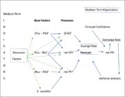
Finally, Harvey (2019) emphasises the role of financial flows to the detriment of trade flows in determining the exchange rate: “(...) currency prices are almost entirely a function of the financial flows (...)” (Harvey, 2019, p.395); “Capital flows set the currency price and then importers and exporters must transact at that price” (Harvey, 2019, p.396); “(...) trade can be imbalanced in equilibrium” (Harvey, 2019, p.409).

Harvey (2019) seems to have underestimated the role of the trade flows. While in this 2019 article he denies its relevance in determining the exchange rate, in Harvey (2009) the expected net exports is one of the three processes that indirectly determine the exchange rate. The author also failed to realise the relevance of structural factors, which persist over time affecting the base factors and processes and, thereby, also indirectly influence the exchange rate. Furthermore, structural factors such as the industrial structure and Dutch Disease have a strong impact on the net exports, reinforcing their importance as a determinant of the exchange rate. The commodity currencies literature provides strong evidence of the importance of net exports in determining the exchange rate.

Harvey (2019) emphasises that trade flows are (almost) offset by financial flows that endogenously finance them via the financial account of the balance of payments, thus marginally affecting the net flow of foreign currency. This does not mean that the net exports is irrelevant in determining the exchange rate. In the Mental Model, what matters is the net effect of balance of payments flows on the exchange rate. Therefore, if trade flows are offset by financial flows, both should be included in the agents’ calculations, justifying the (expected) net exports as one of the processes in the Mental Model.

Furthermore, since confidence affects the intensity of the impact of expectations on the exchange rate - “This vital component [confidence] is often overlooked in discussions of expectations” (Harvey, 2009, p.938), it is possible that the expected net exports is a process that influences another process: the expected net PFI. For instance, if agents are more confident in their expectations about trade flows compared to financial flows, the expectation of an increase in exports can boost the expectation of exchange rate appreciation and, as a consequence, encourage the expected inflow of PFI, even if export revenue is offset by the endogenous outflow of foreign currency. This is because the endogenous flows of international trade finance are mixed in with other financial flows linked to expectations formed with less confidence. This should be the case when the export schedule is dominated by commodities, and the inflow of foreign currency boosted by exports is offset by the outflow of foreign currency that will finance importers, but raises the expected PFI, appreciating the exchange rate from an expected increase in the net exports. The Mental Model would thus be able to explain the case of commodity currencies.

3. EMPIRICAL ESTIMATES OF EXCHANGE RATE MODELS BASED ON THE HARVEY’S MODEL

3.1 Review of empirical literature

Before publishing his ‘Mental Model’ in Harvey (2009), Harvey had already worked on the subject. Harvey (2006) estimated a first difference exchange rate equation for the period 1975-1998, assuming as explanatory variables the interest rate, growth and price differentials between the United States and Germany, as well as a trend variable, the price of energy in dollars and a dummy for the period of German unification. The same equation (except for the dummy) was estimated for the yen-dollar exchange rate. The estimation method was the Ordinary Least Squares. Only the interest rate differential and the trend were statistically significant in both equations.

Although the expectations of foreign exchange market agents are highlighted in Harvey (2006), they are not emphasised in the empirical part of this study. Nevertheless, the role of expectations in determining the exchange rate is central to Harvey (2009). The relationship between expectations and the exchange rate has been researched in the PK literature, but “empirical estimations of their relationship are scarce, with Kaltenbrunner (2011) providing the only one” (Lima; Terra, 2021, p.271).

Kaltenbrunner (2011) estimated a model for Brazil for the period 2003-2009 using the autoregressive vectors method, in which the exchange rate is a function of capital flows to the stock and debt markets (i.e., PFI flows) and expected stock prices and the future interest rate. The latter two variables are proxies for expectations, while PFI flows are ultimately the determinants of the exchange rate in Harvey’s model (2009) .

Lima and Terra (2021) also estimated the relationship between expectations and the nominal exchange rate for Brazil for the period 2002-2017, based on a Harvey’s ‘augmented model’, which includes agents’ expectations about future changes in the exchange rate and the economy’s growth rate. According to the authors, the model that best fits has as arguments all of Harvey’s base factors and processes, in addition to two proxy variables for the agents’ expectations. The estimation method was the distributed lag autoregressive model with error correction.

Barbosa et al. (2017) started from Kaltenbrunner (2015) model to specify and estimate an exchange rate equation using a panel data for 45 countries for the period 1990-2008. The authors sought to explain the determination of the real exchange rate in the long term, although Kaltenbrunner’s (2015) model refers to the nominal exchange rate and emphasises the short-term bias in its determination. The aim of Barbosa et al. (2017) was to include in the model a structural factor that affects the real exchange rate in the long term, namely productivity. The real exchange rate equation estimated by the authors has the following arguments: PFI, domestic and foreign interest rate differential, consumer price index, GDP per capita based on PPP (proxy for productivity) and differential of the liquidity premium of the domestic currency and the dollar.⁶

These three empirical studies, Kaltenbrunner (2011), Lima and Terra (2021) and Barbosa et al. (2017), are based on Harvey’s model (2009) , according to which agents’ expectations about exchange rate changes materialise in the net PFI flow, which determines the nominal exchange rate. However, all three studies include in the estimated equations the explanatory variable PFI which, in turn, is determined by other variables that are also included in the equation as determinants of the exchange rate.

In Kaltenbrunner (2011), the exchange rate depends on the PFI, the expected interest rate and the expected stock prices, but the latter two variables affect the PFI. Lima and Terra (2021) ‘augmented’ Harvey’s model (2009) by introducing the variables of expected economic growth and expected exchange rate change alongside with Harvey’s processes and base factors into the right side of the exchange rate equation. However, in the Mental Model, the expected processes are a function of the expected base factors which, in turn, determine the PFI. Therefore, PFI is the result of agents’ expectations and, in this sense, represents them. However, PFI is included in the equation together with two proxy variables for expectations and with all the base factors and the other two processes. In Barbosa et al. (2017), the PFI is included in the exchange rate equation along with the interest rate differentials and the liquidity premiums of the currencies, but for Harvey (2009), the PFI depends on the interest rate differential and is also affected by changes in the liquidity preference (fourth base factor) which, in turn, alters the liquidity premium differential of currencies.⁷ Furthermore, as explained in section 2.2 of this article, productivity differences among countries are already incorporated into the Mental Model through their effects on base factors and processes. In this sense, structural factors, such as productivity, affect the real exchange rate in the long term through their effects on PFI flows in successive short-term periods.

Therefore, to avoid damaging the estimation results, we chose to estimate an exchange rate equation that directly reflects the Harvey model (2009) , since the effects of variables linked to agents’ expectations and the influences of productivity and other structural factors on the exchange rate are already captured by the base factors and processes of the Mental Model. The specification of the exchange rate model for Brazil, the estimation methodology and the results are below.

3.2 The case of Brazil

Since the stabilisation of prices in Brazil in 1994, a series of innovations have taken place in its financial and foreign exchange markets: financial openness, the development of derivatives and futures markets, new strategies for the central bank to act in the foreign exchange market, etc. (Rossi, 2016). Since then, the exchange rate appreciated for long periods, as well as there were moments of intense exchange rate depreciation and volatility.

Assuming the validity of Harvey’s model (2009) , an equation for the nominal exchange rate was drawn up with the “base factors” of this model as explanatory variables, namely the expected inflation, growth and interest rate differentials between the domestic country and the rest of the world, as well as the relative liquidity of the domestic country’s currency. Due to the difficulty of measuring the expected values of the base factors, it is assumed that the expected values converge to the observed values.⁸ This exchange rate equation is presented below and will be estimated for the Brazilian economy.

The data for the estimation is quarterly. We considered the period for which they are available, the second quarter of 1996 (1996Q2) to the fourth quarter of 2022 (2022Q4).

The data used and the respective sources are: (i) Brazilian basic interest rate (Selic - Central Bank of Brazil (BCB)), (ii) United States (US) basic interest rate (Ipeadata), (iii) Brazilian real GDP (PIB, IBGE), (iv) US current gross domestic product (World Bank) deflated by the Producer Price Index (Bureau of Labour Statistics), (v) Brazilian National Broad Consumer Price Index (IPCA, IBGE), (vi) US Consumer Price Index (Bureau of Labour Statistics) and (vii) average R$/US$ commercial exchange rate (BCB).

Figure 3 shows the series and Table 1 the descriptive statistics:

Figure 3:
Time series

Table 1:
Descriptive statistics

Variables	Minimum	Median	Average	Maximum
exchange	100	230	268.8	561.1
interest diff.	7.924	48.485	52.901	145.028
Inflation diff.	-96.822	26.298	33.685	229.199
Growth diff.	-615.620	25.913	6.093	386.718

• Fonte: Own elaboration; diff. = differential.

3.3 Model Specification and Estimation Methodology

In the model to be estimated, the Brazilian nominal exchange rate is explained by Harvey’s base factors (2009) , which includes a variable to measure the relative liquidity of the real. To test the hypothesis that changes in the liquidity preference in the world and/or in Brazil affect the Brazilian exchange rate, dummy variables (D) were adopted. D is expected to be significant and positive, indicating that in periods of increased uncertainty and liquidity preference in the international market and/or in Brazil, the exchange rate depreciates due to a ‘flight to liquidity’.

We considered: 𝐷𝑅𝑢𝑠𝑠𝑖𝑎 for the Russian crisis, with 𝐷𝑅𝑢𝑠𝑠𝑖𝑎=1 for the third quarter of 1998 and 𝐷𝑅𝑢𝑠𝑠𝑖𝑎 = 0 otherwise; 𝐷𝐿𝑢𝑙𝑎 𝐼 for the speculative attack on the real during the Brazilian presidential election, with 𝐷 𝐿𝑢𝑙𝑎 𝐼=1 for the third and fourth quarters of 2002 and 𝐷𝐿𝑢𝑙𝑎 𝐼=0 otherwise; 𝐷𝑆𝑢𝑏𝑝𝑟𝑖𝑚𝑒 due to the 2008 global financial crisis, with 𝐷𝑆𝑢𝑏𝑝𝑟𝑖𝑚𝑒=1 for the third and fourth quarters of 2008 and 𝐷𝑆𝑢𝑏𝑝𝑟𝑖𝑚𝑒=0 otherwise; and 𝐷𝐶𝑜𝑣𝑖𝑑 for the Covid-19 crisis, with 𝐷𝐶𝑜𝑣𝑖𝑑=1 for the first and second quarters of 2020 and 𝐷𝐶𝑜𝑣𝑖𝑑=0 otherwise. Following Lima and Terra (2021), US data was used as a proxy for global data.

Based on Pesaran and Shin (1998) and Pesaran et al. (2001), the Autoregressive Distributed Lag Model (ARDL) with the Error Correction Term (ECT) was adopted as the estimation method to investigate the presence of short- and long-term vectors. Unlike Vector Autoregressive (VAR) models, which impose the restriction of working with all the variables in the same order of integration, ARDL was chosen because of its ability to deal with a set of variables with different orders of integration, I(0) and I(1). Furthermore, like the VAR models with the ECT, the ARDL model also allows the effects in the short and long term to be assessed separately.

One can write an ARDL Model with ECT as:

$\Delta exchang{e}_t={\alpha }_0-\epsilon \left(exchang{e}_{t-1}+\theta X_{t-1}\right)+\Sigma {\psi }_i\Delta exchang{e}_{t-i}+\Sigma {\phi }_j\Delta X_{t-j}+u_t,$ (1)

where exchange _𝑡 = exchange rate at the time t; X 𝑡 = vector of explanatory variables made up of the interest differential (interest diff.), inflation differential (inflation diff.), growth differential (growth diff.) and the dummy variables 𝐷ℎ for ℎ = (𝑅𝑢𝑠𝑠𝑖𝑎, 𝐿𝑢𝑙𝑎 𝐼, 𝑆𝑢𝑏𝑝𝑟𝑖𝑚𝑒, 𝐶𝑜𝑣𝑖𝑑); 𝛼₀ = intercept; 𝜀 = adjustment speed term; θ = vector of coefficients of the ECT; 𝜓𝑖= set of coefficients of the short-term impact for 𝑖 lags of the change in the exchange rate; φ_𝑗 = vector of coefficients of the short-term impact for 𝑗 lags of the change in the other explanatory variables in the vector X _𝑡; 𝑢_𝑡 = error term.

After estimating the model above, we need to test whether the ECT $\left(ECT=exchang{e}_{t-1}+\theta {\mathit{X}}_{t-1}\right)$ allows us to infer the existence of a long-term linear relationship among the variables in the model. In other words, we would like to know if, after an unexpected shock, the exchange rate adjusts over time in such a way as to maintain a stable linear relationship with the interest, growth and inflation differentials. To do this, we applied the Bounds Test to identify the existence of a long-term relationship among the variables in the model. The test is based on a conventional F statistic to check the joint significance of the cointegration parameters. The null hypothesis of the F-test is that there is no cointegration, i.e, 𝐻0: 𝜀 = θ = 0. After calculating the F-statistic, we compare it with the critical values of the lower and upper limits of the test: (i) if the F-statistic is greater than the critical value of the upper limit, then there is cointegration among the variables; (ii) if the F-statistic is less than the critical value of the lower limit, then the variables are not cointegrated; and, (iii) if the F-statistic is between the two limits, then the cointegration relationship is uncertain. The cointegration relationship also depends on a negative and statistically significant speed of adjustment coefficient. To do this, we will use the Bounds Test t-statistic, with the null hypothesis being that the speed of adjustment coefficient is zero (no cointegration) and the alternative hypothesis being that the coefficient is negative, i.e, 𝐻0: 𝜀 = 0 and 𝐻1: 𝜀 < 0.

Next, we’ll discuss the results of the model.

3.4. Results

The ARDL model makes it possible to estimate a relationship among variables with different orders of integration. However, it is only allowed to include in the model variables with integration order I(0) or I(1), i.e., stationary or with only one unit root, respectively. We therefore carried out unit root tests on the variables of interest and the results are in Appendix I. Our estimates indicate that the exchange rate is non-stationary of order 1, I(1), and the others are stationary, I(0).

The next step is to carry out the cointegration test. Table 2 shows the results of the Bounds Test for small samples:

Table 2:
Result of the Bounds Test for cointegration

Test	Critical values		Test statistics	p-value
	I(0)	I(1)
F	3.351	4.485	4.379	0.055
t	-2.866	-3.783	-0.739	0.936

• Source: Own elaboration.
• Note: The null hypothesis of the F-test is that there is no cointegration, i.e.𝐻0: 𝜀 = θ = 0. The null hypothesis of the t-test is that the speed of adjustment coefficient is zero (no cointegration) and the alternative hypothesis is that the coefficient is negative, i.e. 𝐻0: 𝜀 = 0 and 𝐻1: 𝜀<0.

The results of the Bounds Test do not suggest the existence of a cointegration relationship among the variables in the model. In the first test (𝐹) the result was inconclusive, as the test statistic was higher than the critical value of I(0) and lower than that of I(1). In the second test (𝑡), the model does not cointegrate either, and the test statistic is much higher than the lower critical value of I(0). Therefore, it is not possible to infer a long-term linear relationship among the exchange rate and the interest, growth and inflation differentials. The next step is to estimate Equation (1) from the ARDL model with the ECT. The results are shown in Table 3:

Table 3:
Short- and long-term estimates from the ARDL model with error correction

	Dependent variable: Δexchange t
Variables	Coefficients	Standard Error	t-statistic	p-value
Long-term estimates
Intercept	1014.317	969.203	1.046	0.298
interest diff.s t	-6.173	8.086	-0.763	0.447
Growth diff. t	-7.335	10.423	0.703	0.483
inflation diff. t	-7.671	12.398	0.618	0.537
Short-term estimates
Intercepto	12.600 ***	3.132	4.024	<0.001
Δexchange t-1	0.107	0.090	1.180	0.241
Δexchange t-2	-0.169 **	0.082	-2.052	0.043
Δexchange t-3	0.093	0.080	1.161	0.248
ΔGrowth diff. t	-0.043 ***	0.014	-3.090	0.003
ΔGrowth diff. t-1	0.042 ***	0013	3.248	0.002
Δinflation diff. t	0.074 *	0.040	1.828	0.071
Δinflation diff. t-1	0.084 **	0.041	2.065	0.042
D Lula I	51.420 ***	12.904	3.985	<0.001
D Subprime	22.833 *	12.111	1.885	0.063
D Covid	52.305 ***	11.754	4.450	<0.001
ECT t-1	-0.012 ***	0.003	-4.256	<0.001
Fit statistics and residual tests
R2	0.538
Adjusted R2	0.482
Autocorrelation	7.008 (0.5357)
Normality	5.101 (0.078)
CUSUM	0.526 (0.566)

• Note: An ARDL model (4,0,2,2) selected based on the AIC criterion was estimated. The significance levels are * p < 0.1; ** p < 0.05; *** p < 0.01. The test for serial autocorrelation of the residuals is the Breusch-Godfrey test for up to 8 lags, with the null hypothesis being that there is no autocorrelation of the residuals; the LM statistic and p-value are shown in brackets. The normality test for the residuals is the Jarque-Bera test, with the null hypothesis being that the residuals are normal; the chi-squared statistic and the p-value are shown in brackets. The CUSUM test investigates the stability of the short- and long-term parameters, with the null hypothesis being stability; the S-statistic, p-value in brackets and the test figure are shown in Appendix II.

In the long-term estimates, the coefficients of the three base factors were not statistically significant (Table 3), corroborating the result of the Bounds Test, which indicated the absence of cointegration between the variables in the model.

The short-term estimates (Table 3) indicate the statistical significance, at 5%, of the first difference in the exchange rate lagged by two quarters. The coefficients associated with the growth and inflation differentials, two of Harvey’s three base factors, are also significant at least 10 per cent and show the expected signs. An increase in the first difference of the inflation differential is associated with an increase in the first difference of the exchange rate (increase in exchange rate depreciation) in the period studied, as predicted by the Mental Model. The expected sign for the first difference of the growth differential is ambiguous, since an increase in the growth differential reduces net exports, but stimulates the inflow of foreign currency through DFI and PFI (Harvey, 2009). The Lula I, subprime and covid dummies were significant and positive, indicating that at times of increased uncertainty and liquidity preference in the world and/or in Brazil, the real is neglected and the exchange rate depreciates.

The best ARDL (4, 0, 2, 2) model selected by the AIC criterion excluded the interest rate differential from the short-term estimates. Finally, although the error correction term has a negative sign and is significant at 1%, the results of the long-term estimates and the Bounds Test indicate no cointegration.

These results should be viewed with caution, as the estimated equation does not correspond to a direct representation of Harvey’s mental model (2009), in which the exchange rate is ultimately determined by net flows of PFI. Since these depend on the processes which, in turn, depend on the base factors, by estimating an equation in which the exchange rate is a function of the base factors, we test an indirect representation of the Mental Model. However, the results of the estimations do not allow us to reject the validity of Harvey’s model.

In short, the results found seem to corroborate Harvey’s model or at least do not allow its validity to be rejected, suggesting its adherence to the case of Brazil and the relevance of the conventions and expectations of financial and exchange market agents in determining the exchange rate in the period studied. Behind the process of oscillation of the Brazilian exchange rate appear to be financial flows and decisions by agents with a short-term speculative bias, as suggested in the PK literature. As such, there is a role for economic policy, which should seek to stabilise expectations related to the exchange rate and, as a result, contribute to reducing exchange rate volatility, which is detrimental to investment and economic growth.

4. CONCLUSION

In the PK view, there is no long-term equilibrium exchange rate or pre-defined path, either of appreciation or depreciation, to which the exchange rate would converge in the long term. Post-Keynesians emphasise the short-term and speculative bias in determining the exchange rate, with financial flows being preponderant in this process.

Based on Harvey (2009), we argue that conjunctural and structural factors have an impact on expectations about short-term fluctuations in the exchange rate, determining the PFI which ultimately determines the exchange rate in the short term. In the long term, the exchange rate is indeterminate, being the result of the synthesis of the various factors that affect financial flows in successive short-term periods, from a PK perspective.

This article sought to contribute to the literature by theoretically demonstrating the channel through which structural factors, which act in the short and long term, influence the exchange rate. Factors such as productivity, Dutch Disease, financial integration or the industrial structure of the economy and its trade elasticities, indirectly influence the exchange rate because they impact over successive short periods the base factors and processes of Harvey (2009).

There is also an empirical contribution which, however, did not consider the effects of the structural factors on the exchange rate. The results of the estimation of the exchange rate equation for Brazil, for the period 1996.2-2022.4, corroborate the hypothesis of the validity of Harvey’s model (2009), or at least do not allow it to be rejected. In this case, the relevance of the conventions and expectations of financial market agents in determining the Brazilian exchange rate is highlighted. The formation of the exchange rate, in Brazil, would then depend on short-term and speculative financial flows, as suggested in the PK literature.

There is therefore a role for economic policy, which should seek to influence conventions and stabilise expectations regarding the exchange rate and, as a result, help to reduce exchange rate volatility, which is detrimental to investment and economic growth.

Finally, given that the estimated equation corresponds to an indirect relationship between the exchange rate and its determinant, which, according to Harvey (2006; 2009; 2019), is the net PFI, the results of the estimation should be viewed with caution. However, they were promising in suggesting the speculative and short-term bias in the determination of the exchange rate, opening up space for future research on the subject and indicating the path to be followed.

STATEMENT ABOUT DATA AVAILABILITY

Research data is only available upon request to the researcher.

REFERENCES

• Aguirre, A.; Calderón, C. (2005) Real Exchange Rate Misalignments and Economic Performance, Central Bank of Chile working papers, n. 315: 1-56.
• Andrade, R.P.; Prates, D.M. “Exchange rate dynamics in a peripheral monetary economy”, Journal of Post Keynesian Economics, v.35(3): 399-416.
• Arestis, P, Ferrari-Filho, F, Resende, M.F, Terra, F.B. (2019) “Brazilian monetary and fiscal policies from 2011 to 2017: conventions and crisis”, Challenge. 62: 187-199.
• Balassa, B. (1964) “The purchasing-power parity doctrine: a reappraisal”, The Journal of Political Economy, Chicago, 72(6): 584-596.
• Barbosa, L.O.S; Jayme Jr., F.G.; Missio, F. (2017) “Determinants of the real exchange rate in the long-run for developing and emerging countries: a theoretical and empirical approach”, International Review of Applied Economics, 32(1): 62-83.
• Bergstrand, J.H. (1991) “Structural determinants of real exchange rates and national price levels: some empirical evidence”, The American Economic Review, Nashville, 81(1).
• Bhagwati, J.N. (1984) “Why are services cheaper in the poor countries?”, Economic Journal, 94: 279-286.
• Bresser-Pereira, L.C., Oreiro, J.L., Marconi, N. (2016) Macroeconomia desenvolvimentista: Teoria e Política Econômica do Novo Desenvolvimentismo. Rio de Janeiro: Campus.
• Carvalho, F.J.C. (1984). “Alternative analyses of short and long run in Post Keynesian economics”, Journal of Post Keynesian Economics , 7(2): 214-34.
• Carvalho, F.J.C. (1992) Mr Keynes and the Post Keynesians. Aldershot, UK: Edward Elgar.
• Carvalho, F.J.C. (2018) “Financial flows and the New Developmentalism”, Revista de Economia Política, V.38, 1(150): 115-124.
• Dequech, D. (2011) “Uncertainty: a typology and refinements of existing concepts”, Journal of Economic Issues, v. XLV(3): 621-640.
• Dequech, D. (2022) “Conventions in Keynes’s theory of goods markets: investment and production decisions”, Journal of Post Keynesian Economics , 45(1): 145-167.
• Dow, S. (1993) Money and the economic process. Aldershot, Edward Elgar.
• Fagerberg, J. (1988) “International competitiveness”, Economic Journal, 98(391): 355-74.
• Freeman, C. (1995) “The National System of Innovation in Historical Perspective”, Cambridge Journal of Economics, London, 19(1): 5-24.
• Harvey, J.T. (2006) “Post Keynesian versus neoclassical explanations of exchange rate movements: a short look at the long run”, Journal of Post Keynesian Economics , 161-179.
• Harvey, J.T. (2009) “Currency market participants’ Mental Model and the collapse of the dollar: 2001-2008”, Journal of Economic Issues , v.43(4): 931-949.
• Harvey, J.T. (2019) “Exchange rates and the balance of payments: reconciling an inconsistency in Post Keynesian Theory. Journal of Post Keynesian Economics , v.42(3): 390-415.
• Kaltenbrunner, A. (2011) Currency internationalization and exchange rate dynamics in emerging markets: a post Keynesian analysis of Brazil. Phd Thesis. Department of Economics School of Oriental and African Studies-SOAS, University of London.
• Kaltenbrunner, A. (2015) “A Post Keynesian framework of exchange rate determination: a Minskyan approach”, Journal of Post Keynesian Economics , 38: 426-448.
• Keynes, J.M. (2013a) The General Theory of Employment, Interest and Money. The Collected Writings of John Maynard Keynes, VII, Cambridge University Press.
• Keynes, J.M. (2013b) A tract on monetary reform. The Collected Writings of John Maynard Keynes, IV, Cambridge University Press.
• Lima, L.V.A.; Terra, F.H.B. (2021) “Expectations and exchange rates in a Keynes-Harvey model: an analysis of the Brazilian case from 2002 to 2017”, Review of Keynesian Economics, 9(2): 270-288.
• Paula, L.F.R.; Alves Júnior, A. J. (2000) “External financial fragilty and the 1998-1999 Brazilian currency crisis”, Journal of Post Keynesian Economics , 22(4).
• Pesaran, H.H.; Shin, Y. (1998) “Generalized impulse response analysis in linear multivariate models”, Economics Letters, v. 58, n. 1.
• Pesaran, M. Hashem; Shin, Yongcheol; Smith, Richard J. (2001) “Bounds testing approaches to the analysis of level relationships” Journal of Applied Econometrics, 16(3): 289-326.
• Resende, M.F.C. (2023) Conventions and the Brazilian fiscal policy to face the aftermath of the covid-19 economic crisis: a post keynesian view. Economic Issues, v. 28, part 1: 21-42.
• Resende, M.F.C.; Leone, V.; Torres, D.A.R.; Coleman, S. (2021) “Technological progress, non-price factors competitiveness and changes in trade income elasticities: empirical evidence from South Korea and Hong Kong” European Journal of Economics and Economic Policies: Intervention, V. 18(1): 29-54.
• Rogoff, K. (1996) “The Purchasing Power Parity Puzzle”, Journal of Economic Literature 34(2): 647-668.
• Rossi, P. (2016) Taxa de câmbio e política cambial no Brasil: teoria institucionalidade, papel da arbitragem e da especulação. Rio de Janeiro, ed. FGV.
• Samuelson, P. (1964) “Theoretical notes on trade problems”, Review of Economics and Statistics, Cambridge, 46(2):145-154, May.

• 1
  There is internal equilibrium when the natural rate of unemployment prevails and external equilibrium when the balance of payments constraint is satisfied (Aguirre; Calderón, 2005).
• 2
  We are considering chronological time as the element that distinguishes between the short and long terms. For an analytical distinction between the short and long terms from the point of view of many branches in economics, see Carvalho (1984).
• 3
  Kaltenbrunner (2011, p.264) finds a high and positive correlation between nominal and real exchange rates in Brazil. She uses price rigidity to explain this picture, without explaining that rigidity stems, among other factors, from the absence of arbitrage with non-tradable goods.
• 4
  Dequech (2022) also gives other reasons for the emergence of conventions in a context of uncertainty.
• 5
  Structural factors have different effects on the processes and base factors of developed and developing countries, and are an influence on exchange rate depreciation (appreciation) in developing (developed) ones.
• 6
  Barbosa et al. (2017) used four variables in the estimated equation as a proxy for the liquidity premium differential.
• 7
  In the literature of currencies hierarchy (CHL) the liquidity premium (l) of each currency is fixed (Andrade; Prates, 2013; Kaltenbrunner, 2015). The CHL is based on Keynes’ asset choice model (2013a). However, to Keynes the values of the attributes of any asset oscillate with changes in expectations, including l. To Keynes (2013a), the interest rate is the premium for relinquishing liquidity. Thus, if the interest rate fluctuates, so does this premium. The degree of liquidity of the currency is fixed in the short run, but its l is not. When uncertainty changes, society’s appreciation (or desire) for liquidity also changes, altering the interest rate and the currency liquidity premium. In chapter 17 of Keynes (2013a), l ₃ is the liquidity premium of money and Keynes concludes that the ‘own rate of interest’ of money falls more slowly than the own rates of interest of other assets when output increases, suggesting that l ₃ can change: “(...) since l ₃ (...) is either fixed or falling more slowly than q₁ or -c₂ , (...)” (Keynes, 2013a, p.228). How can we explain the flight to quality that Harvey (2009, p.936) comments on, without changes in the liquidity premiums of currencies, or changes in the premium differential, considering that it is unlikely that the q and c attributes of assets can change intensely in the space of a few days? Instead of assuming that the range of oscillation of the liquidity premium of the more liquid currencies is greater than that of the less liquid currencies, the CHL assumes that the liquidity premium differential of the currencies is fixed and that the perceived risk of the agents is what oscillates and will be offset by changing the sum of the attributes a+q-c (Andrade; Prates, 2013, p. 411).
• 8
  Harvey (2006) also uses the observed values of the explanatory variables in his exchange rate equation.
• JEL Classification:
  E12; F31; F32.

APPENDIX I

Unit root test results

Variables	ADF	KPSS	PP
exchange	-1.64	0.16**	0.85
interest diff.	-3.52**	0.08	0.02**
Growth diff.	-3.73**	0.09	0.01**
Inflation diff.	-4.32***	0.06	0.01**
Δexchange	-7.00***	0.10*	0.01**
Δ interest diff.	-6.03***	0.05	0.01**
Δ Growth diff.	-11.12***	0.07	0.01**
Δ inflation diff.	-13.26***	0.06	0.01**

• Source: Own elaboration.
• Note: Significance levels are * p<0.1; ** p<0.05; *** p<0.01. Three-unit root tests were carried out to identify the stationarity of the variables: Augmented Dickey-Fuller (ADF), Kwiatkowski-Phillips-Schimidt-Shin (KPSS) and Phillips-Perron (PP). The null hypotheses of the ADF and PP tests are non-stationarity, while that of the KPSS test is stationarity. The ADF test considered constant and trend with variables in level and without constant and trend in first difference.

APPENDIX II

Test CUSUM

Publication Dates

• Publication in this collection
  10 Nov 2025
• Date of issue
  2025

History

• Received
  15 Feb 2024
• Accepted
  19 Dec 2024