Twins in relativistic spacetimes: dispelling some misconceptions

Gêmeos em espaços-tempos relativísticos: dirimindo algumas concepções errôneas

Abstract

In contrast to Newtonian physics, there is no absolute time in relativistic (Lorentzian) spacetimes. This immediately implies that two twins may, in general, age differently. For this to happen, there must be, of course, some asymmetry between their worldlines, along which the elapsed proper times are evaluated; such asymmetry might not be, however, so intuitively apparent. Our main aim is to recollect, in a concise didactic manner, some not so well-known results and derive novel ones, from a modern, geometrical, covariant standpoint, which aim to clarify the issue and dispel some related misconceptions. First, we recall that: (i) the original “twin paradox” may be perfectly dealt with in special relativity (physics in a flat spacetime) and does not necessarily involve an accelerated twin. Then we explore the issue of differential aging in general relativity (physics in a curved background), in the prototypical case of the vacuum Schwarzschild spacetime, by considering several couples of twins. In this context, we show that: (ii) it is not true that a twin which gets closer to the Schwarzschild horizon, by being subject to a stronger gravitational field, where time sort of slows down, should always get younger than a twin that stays further away, in a region of weaker gravitational field, and (iii) it is also false that an accelerated twin always returns younger than a geodesic one. Finally, we argue that (iv) in a generic spacetime, there is no universal correlation between the phenomena of differential aging and the Doppler effect. Two particularly pedagogical resources provided are a glossary of relevant terms and supplementary Python notebooks, both in a Github repository.

Keywords
Relativistic differential aging; twin paradox; vacuum Schwarzschild spacetime

Resumo

Em constraste com a física newtoniana, não há um tempo absoluto em espaços-tempos relativísticos (lorentzianos). Isso implica, imediatamente, que dois gêmeos podem, em geral, envelhecer diferentemente. Para que isso ocorras, deve haver, claro, alguma assimetria entre as suas linhas de universo, ao longo das quais os tempos próprios transcorridos são avaliados; tal assimetria pode, contudo, não ser tão óbvia. Nosso objetivo principal é coligir, de uma maneira didática, alguns resultados não tão bem conhecidos e deduzir outros novos, a partir de um ponto de vista moderno, geométrico, covariante. que visam esclarecer a questão e dirimir algumas concepções errôneas correspondentes. Primeiro, relembramos que: (i) pode-se lidar, perfeitamente, com o “paradoxo dos gêmeos” original na relatividade especial (física em um espaço-tempo chato) e que ele não necessariamente envolve um gêmeo acelerado. A seguir, exploramos a questão do envelhecimento diferencial na relatividade geral (física em um fundo curvo), no caso prototípico do espaço-tempo de Schwarzschild do vácuo, considerando vários pares de gêmeos. Nesse contexto, mostramos que: (ii) não é verdade que um gêmeo que se aproxima mais do horizonte de Schwarzschild, ao estar sujeito a um campo gravitacional mais forte, onde o tempo, de certa forma, passa mais devagar, deveria sempre ficar mais jovem do que um gêmeo que se mantém mais longe, em uma região de campo gravitacional mais fraco, e (iii) também é falso que um gêmeo acelerado sempre retorno mais jovem que um geodésico. Finalmente, argumentamos que (iv) em um espaço-tempo genérico, não há uma correlação universal entre os fenômenos de envelhecimento diferencial e de efeito Doppler. Dois recursos particularmente pedagógicos fornecidos são um glossário de termos relevantes e notebooks em Python, ambos disponíveis em um repositório Github.

Keywords
Envelhecimento diferencial relativístico; paradoxo dos gêmeos; espaço-tempo de Schwarzschild do vácuo

1. Introduction

In the highly acclaimed Interstellar blockbuster movie from 2014, characters Cooper and Amelia visit the ocean world planet Miller, close to the black hole Gargantua, for a few hours, while their fellow Romilly stays in the spaceship Endurance, in orbit around the black hole. When they meet again, Romilly has aged about 23 years! [¹] This is usually explained by stating that, near massive bodies, time slows down. In another classic movie, Planet of the Apes, from 1968, a crew of astronauts returns to an Earth 2 millennia older, after a space voyage that lasted for them only about a year! This is usually attributed to the fact that accelerated bodies grow younger as compared to inertial or geodesic ones. In this article, we will show, inter alia, that those types of explanation are not universally valid.

The latter issue, related to the Planet of the Apes movie, is frequently referred to in the literature as the so-called “twin paradox”. We would like, from the outset, to spell out a misunderstanding as regards the use of the term “paradox”: of course, there is no legitimate logical paradox at all, but only a seemingly contradictory result, as viewed from a Newtonian or special relativistic framework (cf. Secs. 2 and 3).

In this article, we study the relative aging of several relevant pairs of twins, briefly in special relativity (SR) and more systematically in the particular context of vacuum Schwarzschild spacetime of general relativity (GR), and thereby we provide counterexamples to two recurring impressions that students might infer from the popularization literature or even some textbooks: (1) that a geodesic twin always gets older than an accelerated one (e.g. [², p. ³⁴], [³, p. 21], [⁴, p. 3-4]), and (2) that a twin which travels closer to a matter source necessarily gets younger than one which stays further away (e.g. [⁵, p. 253], [⁶, p. 55, 118], [⁷, p. 7, 8 and 33].

The structure of the article is as follows. In Sec. 2, in a relativistic context, we present some fundamental concepts related to the loose (and otherwise ambiguous) notion of an observer, show their relevance for the correct specification of any idea of time interval and present the concrete hypotheses underlying the differential aging issue and its resolution in an arbitrary spacetime. In Sec. 3, we very briefly recall a flat spacetime where the asymmetry which explains the differential aging between two smooth observers may not be ascribed to differences in (proper) acceleration. In Sec. 4, we describe the four kinds of (intersecting) twins we will consider in vacuum Schwarzschild spacetime: an accelerated static Killing observer and three (not necessarily smooth) geodesic observers. In Sec. 5, we derive the ratios of proper times and display the corresponding plots. In Sec. 6, we argue that, given two arbitrary twins in a generic (curved) spacetime, there is no clearcut relation between their differential aging and the corresponding Doppler shift between them. Finally, in Sec. 7, we conclude with a discussion of the main results and some future perspective.

Some of our conventions are: (i) the signature for the metric is “mostly positive”, i.e., (−1, 1, 1, 1); (ii) we will systematically set Newton’s gravitational constant G_N and the vacuum speed of light equal to one: G_N≡c≡ 1; (iii) Greek indices run from 0 to 3, and Latin ones from 1 to 3.

2. Lorentzian Spacetimes and Differential Aging in General

Newtonian physics is developed such that there is, in a given background manifold, a notion of absolute time, which may, naively speaking, be identified with a privileged scalar field in such a manifold.¹ Thus, given two events, 𝒫 and 𝒬, there is an absolute time interval assigned to them, ΔT(𝒫, 𝒬) := T(𝒬) − T(𝒫), irrespective of the observers (𝒪₁, 𝒪₂, …) which are present there. This expresses the absence or rather the meaninglessness of any differential aging (or “twin paradox”) in such setting.

With the Newtonian case briefly addressed, we now turn to a Lorentzian spacetime². Following the lead of [¹²], we urge the reader to distinguish among the concepts of instantaneous observer, observer, reference frame, (not to be confused with either a coordinate system or a tetrad (field)), which are crucial for a definition of any kind of time interval, and therefore for a perfect understanding of the issue of differential aging (or, as an abuse of language, “twin paradox”).

Let there be given two infinitesimally close events x^α and x^α + dx^α. Whenever we want to refer to an infinitesimal time interval measurement between those events, be it in the context of special relativity (locally flat, Minkowski spacetime) or general relativity (curved spacetime proper), there must be, at least implicitly, an associated instantaneous observer (𝒫, u^α), such that the mentioned time interval refers to the proper time assigned by this very instantaneous observer to the infinitesimal displacement dx^α, according to:

(1) $$dT(d{x}^{\alpha },u^{\alpha })\text{:=}-d{x}^{\alpha }{u}_{\alpha }.$$

This is to be contrasted, for instance, with the curvature tensors (Riemann, Ricci, Weyl and Einstein), at a given event, which depend only on the metric and its derivatives, but not on any instantaneous observer. Likewise, if we want to refer to the time interval between two events 𝒮 and 𝒜, along a given observer 𝒪, parametrized as γ^α(τ), we mean, of course:

(2) $$\mathrm{\Delta }\tau [{𝒪}_{𝒮\to 𝒜}]\text{:=}{\int }_{{𝒪}_{𝒮\to 𝒜}}\sqrt{-g_{\alpha \beta }{\stackrel{.}{\gamma }}^{\alpha }(\tau ){\stackrel{.}{\gamma }}^{\beta }(\tau )}\mathit{d}\tau .$$

The concrete setting for the differential aging issue, in any given spacetime, demands, for its very formulation, the consideration of two arbitrary observers, 𝒪₁ and 𝒪₂, geodesic or accelerated, which meet, at least, at two events, 𝒮 and 𝒜 (cf. Fig. 1), so that they can compare their corresponding elapsed proper times between those events, Δτ_{O1,S →A} and Δτ_{O2,S →A}, and thus ascertain whether they are different, i.e., whether there is any differential aging; if that is the case, it would be expedient to somehow account for it.

Figure 1
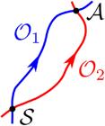
Two relevant observers, 𝒪₁ and 𝒪₂, meeting at events 𝒮 (start) and 𝒜 (arrival), for the setting of the differential aging issue in an arbitrary spacetime (ℳ,g_αβ).

The generic explanation, in any spacetime, for such a Newtonian unexpected result for the twins, rests simply on three premises:

1. the validity of the clock hypothesis, as most clearly exposed by Rindler [¹³], which states that the physically relevant time is defined by the proper time of ideal (point) clocks independently of their geodesic or accelerated motion and of their location. This amounts to disregarding any explicit, direct modification of the inner workings of an ideal clock, such as an atomic one, upon the curvature tensors of the underlying neighborhood. Due to the typical dominance of the electric force over the gravitational tidal forces, this is practically always valid [¹⁴];

2. the non-exact character of the infinitesimal interval dT in Equation (1) or, equivalently, the dependence of the elapsed proper time integral Δτ in Equation (2) on the observer connecting two given, fixed events. Alternatively, in contrast to the Newtonian case, there is no absolute time assigned to events (apart from a universal offset);

3. the ultimate existence of an asymmetry (metrical³ or topological) between the twins, which implies distinct values for Equation (2).

3. Special Relativity: Flat Spacetimes

By special relativity we mean physics in a spacetime with vanishing Riemann curvature tensor, i.e., in a flat spacetime (usually called a Minkowski spacetime). The underlying manifold may have the trivial topology of ℝ⁴ or an “exotic” one. If one chooses the trivial one, as depicted for two dimensions in panel (a) of Fig. 2, it is obvious that, given two events, 𝒮 and 𝒜 in its future, then there is a unique (smooth) geodesic observer connecting such events, 𝒪₁ in the panel, for which the proper time interval Equation (2) is maximal: any other observer, such as a broken (non-smooth) geodesic (𝒪₂ in the panel) or a (smoothly) accelerated one, ages more than 𝒪₁. Thus, in this case, the asymmetry which explains the differential aging is due to an acceleration (impulsive or not). Sometimes, people try to extrapolate this to the effect that: (i) an acceleration is always necessary for the asymmetry and (ii) an observer which is a smooth geodesic always ages less than any other one (be it a broken geodesic or a smoothly accelerated one). This can be readily refuted by considering the cylindrical Minkowski spacetime in panels (b) and (c) of Fig. 2 [cf. [¹⁵, ¹⁶, ¹⁷, ¹⁸]]. Indeed the observer 𝒪₂ in such panels is also a smooth geodesic and of course ages less than observer 𝒪₁.

Figure 2
Flat spacetimes: (a) standard, simply connected, Minkowski spacetime. (b) cylindrical Minkowski spacetime (c) covering flat spacetime corresponding to (b).

4. General Relativity: Vacuum Schwarzschild Spacetime

For the vacuum Schwarzschild spacetime⁴, we will work within the usual (symmetry-adapted) spherical coordinate chart, x^α: = (t, r, θ, φ), in which the line element is given by

(3) $$\begin{array}{l}\begin{array}{cc}d{s}^2=-\left(1-\frac{2M}{r}\right)d{t}^2& \end{array}\\ \begin{array}{cc}& +{\left(1-\frac{2M}{r}\right)}^{-1}d{r}^2+r^{2}d{\theta }^2+r^2{\sin }^2\theta d{\phi }^2,\end{array}\end{array}$$

where M is the mass. Such a metric satisfies Einstein’s field equations of general relativity, with a vanishing energy-momentum tensor and a vanishing cosmological constant, for the following domain of the coordinate functions: −∞ < t < ∞, 0 < r < ∞, 0 < θ, π, 0 < φ < 2π. This is the single coordinate system we will use throughout the article, restricted, in fact, to the region outside the horizon: 2M < r < ∞⁵, though we could easily extend the results to the region inside. The congruence of static Killing observers defines a sort of privileged fiducial reference frame (comoving with the aforementioned chart), which is irrotational, rigid (expansionless and shear-free), but non-geodesic (cf. Sachs1977). Its proper acceleration is

(4) $$a^{\alpha }=\frac{M}{r^2}{\delta }_1^{\alpha }\mathit{}⟹\mathit{}a=\frac{M}{r^2\sqrt{1-2M/r}}.$$

We can choose a corresponding instantaneous observer ((t, r, θ, φ),(dt/dτ, 0)) whose infinitesimal proper time is, of course,

(5) $$d{\tau }_{𝒦}=\sqrt{\left(1-\frac{2M}{r_{𝒦}}\right)}dt.$$

For such a static observer, 𝒦 say (cf. Fig. 3), with fixed spatial coordinates (r = r_𝒦, θ = θ_𝒦, φ = φ_𝒦), and, along it, two arbitrary events 𝒮:(t = t_𝒮, r = r_𝒮 = r_𝒦, θ = θ^𝒮 = θ_𝒦, φ = φ_𝒮 = φ_𝒦) and 𝒜:(t = t_𝒜, r = r_𝒜 = r_𝒦, θ = θ_𝒜 = θ_𝒦, φ = φ_𝒜 = φ_𝒦), with 𝒜 in the future of 𝒮, i.e., t_𝒜 > t_𝒮. Of course, the corresponding time coordinate interval between such events is simply

Figure 3
The fountain of youth region (in yellow) in the Schwarzschild spacetime, relative to a static Killing observer 𝒦: (a) spacetime diagram (cylindrical shell). (b) spatial projection onto the equatorial 2-plane θ = π/2 (annulus).

(6) $$\mathrm{\Delta }t(𝒮,𝒜)=t_{𝒜}-t_{𝒮},$$

and the corresponding proper time interval, along 𝒦 [cf. (5)], is

(7) $$\mathrm{\Delta }{\tau }_{{𝒦}_{𝒮\to 𝒜}}=\sqrt{\left(1-{\displaystyle \frac{2M}{r_{𝒦}}}\right)}\mathrm{\Delta }t(𝒮,𝒜).$$

Along an arbitrary observer, from Equation (3), the corresponding elapsed infinitesimal proper time may be written as

(8) $$d{\tau }^2=\mathrm{}\left(1-2M/r\right)d{t}^2-{\left(1-2M/r\right)}^{-1}d{r}^2-r^2\left(d{\theta }^2+{\sin }^2\theta d{\phi }^2\right).$$

The time coordinate t is well defined within the whole exterior region (2M < r < ∞), and so we can also parametrize the mentioned arbitrary observer by a static Killing observer’s proper time; thus, by using (5) and (8), we have

(9) $$\begin{array}{l}d{\tau }^2=\mathrm{}d{\tau }_{𝒦}^2\{{\displaystyle \frac{1-2M/r}{1-2M/r_{𝒦}}}-{\displaystyle \frac{1}{1-2M/r}}{\left({\displaystyle \frac{dr}{d{\tau }_{𝒦}}}\right)}^2\mathrm{}-\mathrm{}{r}^2{[{\left({\displaystyle \frac{d\theta }{d{\tau }_{𝒦}}}\right)}^2+{\sin }^2\theta \left({\displaystyle \frac{d\phi }{d{\tau }_{𝒦}}}\right)]}^2\}.\end{array}$$

Inasmuch as, by definition, an observer is timelike, the expression within braces must be positive. However, it is not guaranteed in general that such an expression is definitely greater (or smaller) than 1 and thus we cannot state a priori that an arbitrary observer gets older (or younger) than a static one, 𝒦.

Nevertheless, we will now show that there is a generous collection of observers, say 𝒴, which will become younger than a corresponding static observer 𝒦. To that end, given a static observer 𝒦, with radius r_K, choose a distinct observer which carries out an arbitrary trip not further than 𝒦, i.e., with r≤r_𝒦 everywhere, which implies (1 − 2M/r)/(1 − 2M/r_𝒦) ≤ 1. We now see that the first term in the braces of Equation (9) is already less than 1 and therefore

(10) $$d{\tau }_{𝒴}<d{\tau }_{𝒦}.$$

The total proper time is given by the integral of dτ_𝒴 from 𝒮 up to 𝒜 and thus, provided Equation (10) holds all along, we conclude

(11) $$\mathrm{\Delta }{\tau }_{𝒴}\le \mathrm{\Delta }{\tau }_{𝒦}$$

and the equality holds only for 𝒴 = 𝒦 (otherwise the spatial coordinates would vary at some interval and we would have dτ_𝒴 < d_τ𝒦 in this interval). In other words, every arbitrary (non-static) observer 𝒴, starting at 𝒮 and arriving at 𝒜, that travels everywhere inside a (4-dimensional) cylindrical shell (annulus) 2M < r≤r_𝒮 = r_𝒜 = r_𝒦 in Schwarzschild spacetime returns younger than the corresponding static Killing observer at r_K: we find a fountain of youth region of spacetime, with respect to the particular observer 𝒦 [cf. panel (a) of Fig. 3]! In the spatial projection, the fountain of youth is a spherical shell covering the region 2M < r≤r_𝒦 [cf. panel (b) of Fig. 3].

In this sense, in relation to the Killing observer, going closer to the source indeed will cause our clock to run slower. However, the argument does not hold if the observer wanders outside the fountain of youth, relative to 𝒦, since we would typically have additional kinetic terms of varying coordinates which would prevent ascertaining the value for the ratio dτ/dτ_𝒦; therefore, we should be careful when employing this kind of general claim. Below (see Subsec. 5.6) we will provide a concrete example illustrating that the fountain of youth region is not a fountain of youth relative to general observers which travel outside it.

To deal with more quantitative results for differential aging, we will consider the four typical observers 𝒦, 𝒰, 𝒟 and 𝒞 and some related events, which are listed in Table 1 and represented in Fig. 4. Thus the twins to be dealt with in the comparison of their corresponding proper times are: (𝒰, 𝒦), (𝒟, 𝒦), (𝒟, 𝒰), (𝒞, 𝒦), (𝒰, 𝒞), and (𝒟, 𝒞). It is worth mentioning that Sokolowski [¹⁹] examined the cases involving only observers 𝒦, 𝒰 and 𝒞, illustrating the results in the form of a numerical table. He stated that 𝒰 describes the longest possible curve between the events 𝒮 and 𝒜 since the geodesic followed by him contains no conjugate points [²⁰, ²¹] in this interval. Later [²²], he noticed that this result is valid only for the neighborhood of the fiducial curve. We will now characterize all four such observers in more detail.

Table 1
Symbols and description of relevant observers and events.

Symbol	Description
𝒦	Static Killing observer
𝒴	Younger observer, with respect to 𝒦
ℛ	Generic radial geodesic observer $[\dot{\phi }(\tau )\equiv 0]$
𝒰	Radial geodesic observer launched upward [$\stackrel{.}{r}\left(𝒮\right)>0$], reaching a halt (stop) event ℋ
𝒟	Radial geodesic observer, released from rest [$\stackrel{.}{r}\left(𝒮\right)=0$], falling initially downward, reaching a bouncing event ℬ
𝒞	Circular geodesic observer
𝒮	Start (departure) event
𝒜	Arrival (“reunion”) event
𝒫	Generic pause event on the generic radial geodesic observer $\left[\stackrel{.}{r}\left(𝒫\right)=0\right]$: ℋ on 𝒰, or 𝒮 and 𝒜 on 𝒟
ℋ	Halt (stop) event [$\stackrel{.}{r}\left(\mathscr{H}\right)=0$] on 𝒰
ℬ	Bouncing event [${lim}_{\tau \to \tau {\left(ℬ\right)}_{+}}\stackrel{.}{r}\left(\tau \right)=-{lim}_{\tau \to \tau {\left(ℬ\right)}_{-}}\stackrel{.}{r}\left(\tau \right)$] on 𝒟

Figure 4
Diagrams for the six couples of twins considered in the vacuum Schwarzschild spacetime; the left and right sides of each panel, from (a) to (f), show, respectively, the corresponding spacetime diagram and the spatial projection onto the equatorial 2-plane θ = π/2. (a) the couple 𝒰 and 𝒦. (b) the couple 𝒟 and 𝒦. (c) the couple 𝒟 and 𝒰. (d) the couple 𝒞 and 𝒦. (e) the couple 𝒰 and 𝒞. (f) the couple 𝒟 and 𝒞.

4.1. Geodesic observers

In a Lorentzian spacetime (ℳ, g_αβ(x^μ)), its geodesics can be thought of as the extremal curves of the variational problem associated with the Lagrangian

(12) $$ℒ(x^{\mu }(\tau ),{\stackrel{.}{x}}^{\mu }(\tau ))=\frac{1}{2}{g}_{\alpha \beta }(x^{\mu }(\tau )){\stackrel{.}{x}}^{\alpha }(\tau ){\stackrel{.}{x}}^{\beta }(\tau ),$$

where the parameter τ for the extremal curves turns out to be any affine parameter. For timelike geodesics, it can then be chosen, without any loss of generality, as its proper time. Thus, since the Lagrangian itself is a constant of motion, it is apparent, on the geodesics, to be normalized such that

(13) $$2ℒ(x^{\mu },{\stackrel{.}{x}}^{\mu })=-1.$$

Due to the spherical symmetry of (3), we can, again without any loss of generality, restrict our study to equatorial geodesics θ ≡π/2, the associated x²:= θ component of the geodesic equation being identically satisfied.

The (covariant) canonical momentum associated to coordinate x^α is defined by

(14) $$p_{\alpha }\text{:=}\frac{\partial ℒ}{\partial {\stackrel{.}{x}}^{\alpha }}=g_{\alpha \beta }(x^{\mu }){\stackrel{.}{x}}^{\beta }.$$

Taking into account (3), since the coordinates x⁰:=t and x³:=φ are ignorable (cyclic) for the Lagrangian (12), the corresponding canonical momenta are constants of motion:

(15a) $$p_0=-\left(1-{\displaystyle \frac{2M}{r}}\right)\stackrel{.}{t}\text{=:}-E=\text{const}<0,$$

(15b) $$p_3=r^2{\sin }^2\theta \stackrel{.}{\phi }=r^2\stackrel{.}{\phi }\text{=:}L=\text{const},$$

with E interpreted as a sort of energy (per mass) of the geodesic particle, whereas L is a sort of its azimuthal angular momentum (also per mass). For these equatorial geodesics, we now use (3) into (13) to obtain

$$-\left(1-\frac{2M}{r}\right){\stackrel{.}{t}}^2+{\left(1-\frac{2M}{r}\right)}^{-1}{\stackrel{.}{r}}^2+r^2{\stackrel{.}{\phi }}^2=-1,$$

and then (15a) and (15b) to get rid of $\stackrel{.}{t}$ and $\stackrel{.}{\phi }$, leading us to

(16) $${\left(\frac{dr}{d\tau }\right)}^2=\left(1-2M/r\right)\left(-1+\frac{E^2}{1-2M/r}-\frac{L^2}{r^2}\right)\ge 0.$$

This is the well-known relativistic analog of the reduction of the Keplerian radial problem to a one-dimensional problem [²³, ²⁴]; in fact (16) can be rewritten as

(17) $${\left(\frac{dr}{d\tau }\right)}^2=E^2-V(r),$$

where V(r) plays the role of an effective potential, defined by [²⁵, Sec. 9.3] [²⁶, Sec. 5.4]:

(18) $$V(r;M,L):=\left(1-\frac{2M}{r}\right)\left(1+\frac{L^2}{r^2}\right).$$

The relevant parametric geodesics equations can be cast in the form

(19a) $${\displaystyle \frac{d\tau }{dr}}=\pm {\left[E^2-V(r;M,L)\right]}^{-1/2},$$

(19b) $${\displaystyle \frac{dt}{d\tau }}={\displaystyle \frac{E}{1-2M/r}},$$

(19c) $${\displaystyle \frac{d\phi }{d\tau }}={\displaystyle \frac{L}{r^2}},$$

(19d) $${\displaystyle \frac{dt}{dr}}=\pm E{\left(1-{\displaystyle \frac{2M}{r}}\right)}^{-1}{\left[E^2-V(r;M,L)\right]}^{-1/2}.$$

4.1.1. Generic radial geodesic observers ℛ

For radial geodesics, L = 0, (19) simplifies to

(20a) $${\displaystyle \frac{d\tau }{dr}}=\pm {\left(E_{ℛ}^2-1+{\displaystyle \frac{2M}{r}}\right)}^{-1/2},$$

(20b) $${\displaystyle \frac{dt}{d\tau }}={\displaystyle \frac{E_{ℛ}}{1-2M/r}},$$

(20c) $${\displaystyle \frac{d\phi }{d\tau }}=0,$$

(20d) $${\displaystyle \frac{dt}{dr}}=\pm E_{ℛ}{\left(1-{\displaystyle \frac{2M}{r}}\right)}^{-1}{\left(E_{ℛ}^2-1+{\displaystyle \frac{2M}{r}}\right)}^{-1/2},$$

where now the energy parameter is denoted by E_ℛ.

The only branches (arcs) of radial geodesic observers we will consider in this subsubsection are those that are infalling; they may be thought of as constituting either the infalling branch ${𝒰}_{\mathscr{H}\to 𝒜}$ of observer 𝒰, or the infalling branch ${𝒟}_{𝒮\to ℬ}$ of observer 𝒟. In any case, there is an event 𝒫 at which the radial observer is momentarily paused (at rest) with respect to a corresponding static Killing observer, $\stackrel{.}{r}(𝒫)=0$, viz.: for ${𝒰}_{\mathscr{H}\to 𝒜}$, the halt event ℋ, or, for ${𝒟}_{𝒮\to ℬ}$, the start event 𝒮 (cf. Fig. 4).

At such particular pause events 𝒫 (on ℛ) we thus have, from (20a), the following constraint

(21) $$0<E_{ℛ}=E_{𝒫}:=\sqrt{1-2M/r_{𝒫}}<1\iff r_{𝒫}=\frac{2M}{1-E_{𝒫}^2}.$$

Equations (20a) and (20d) can be integrated into a closed but complicated form. However, a much simpler procedure, following the lead of Misner, Thorne, and Wheeler [²⁴] (cf. also Chandrasekhar [²³]), consists in defining a new coordinate η as

(22) $$0\le \eta :=\arccos \left(\frac{2r}{r_{𝒫}}-1\right)\le \pi ,$$

so η = 0 for r = r_𝒫 (and, were we to extend the arc up to the singularity r = 0, then η = π). Thus

(23) $$r=\frac{r_{𝒫}}{2}(1+\cos \eta )=r_{𝒫}{\cos }^2(\eta /2).$$

It is also convenient to define the value η = η_h at the associated static black hole horizon radius r_h:= 2M, such that

(24) $${\eta }_h=2\arcsin E_{𝒫}>0.$$

In terms of η, it is not difficult to show that

(25) $$\frac{d\tau }{d\eta }=\sqrt{\frac{r_{𝒫}^3}{2M}}{\cos }^2(\eta /2),$$

and

(26) $$\frac{dt}{d\eta }=E_{𝒫}\sqrt{\frac{r_{𝒫}^3}{2M}}\frac{{\cos }^4(\eta /2)}{{\cos }^2(\eta /2)-{\cos }^2({\eta }_h/2)}.$$

Integration of (25) and (26), from 𝒫 : (η_𝒫 = η(r_𝒫) = 0) to a generic event (to the future of 𝒫) ℰ:(_{ηℰ = η(rℰ}) > 0), gives, respectively,

(27) $$\mathrm{\Delta }{\tau }_{{ℛ}_{𝒫\to ℰ}}(M,r_{𝒫},r_{ℰ})=\sqrt{\frac{r_{𝒫}^3}{8M}}({\eta }_{ℰ}+\sin {\eta }_{ℰ}),$$

and

(28) $$\begin{array}{l}\mathrm{\Delta }{t}_{{ℛ}_{𝒫\to ℰ}}(M,r_{𝒫},r_{ℰ})\\ =E_{𝒫}\sqrt{{\displaystyle \frac{r_{𝒫}^3}{2M}}}{F}_1({\eta }_{ℰ},E_{𝒫})+2M{F}_2({\eta }_{ℰ},{\eta }_h),\end{array}$$

where

(29a) $$F_1({\eta }_{ℰ},E_{𝒫}):={\displaystyle \frac{1}{2}}({\eta }_{ℰ}+\sin {\eta }_{ℰ})+{\eta }_{ℰ}(1-E_{𝒫}^2),$$

(29b) $$F_2({\eta }_{ℰ},{\eta }_h):=\ln \left[{\displaystyle \frac{\tan ({\eta }_h/2)+\tan ({\eta }_{ℰ}/2)}{\tan ({\eta }_h/2)-\tan ({\eta }_{ℰ}/2)}}\right].$$

4.1.2. Generic circular geodesic observers 𝒞

The roots of dV/dr = 0 or, equivalently,

(30) $$M{r}_{𝒞}^2-L_{𝒞}^2{r}_{𝒞}+3M{L}_{𝒞}^2=0,$$

i.e.,

(31) $$r_{𝒞\pm }=\frac{L_{𝒞}^2}{2M}\left(1\pm \sqrt{1-\frac{12M^2}{L_{𝒞}^2}}\right),$$

are potential candidates for the radii of circular geodesics orbits; for them to correspond to actual circular geodesics, they have to be greater than 2M. This is satisfied if and only if $L_{𝒞}^2\ge 12M^2$, implying, of course, the reality and positivity of the roots. The larger root, r_C+, corresponds to a stable circular orbit (local minimum of V) and the smaller root, r_C–, corresponds to an unstable circular orbit (local maximum of V). For the minimum value $L_{𝒞}^2/M^2=12$ we have r_𝒞± = 6M, which is the infimum for the radius of a stable circular orbit: r_𝒞+ ≥ 6M. The infimum for the radius of an unstable circular orbit corresponds to L_𝒞 → ∞; in this case, $12M^2/L_{𝒞}^2\to 0$ and $\sqrt{1-12M^2/L_{𝒞}^2}\approx 1-6M^2/L^2$, so r_𝒞− > 3M. Thus, there exist unstable circular geodesic orbits for 3M < r_𝒞− ≤ 6M while for 6M < r_{𝒞 +} < ∞ we do have stable geodesic circular orbits.

Let us now find the period of the orbit in terms of proper and coordinate time. Solving (30) for $L_{𝒞}^2$, we find the relation between the angular momentum for any circular geodesic and its radius:

(32) $$L_{𝒞}^2=\frac{M{r}_{𝒞}}{1-3M/r_{𝒞}}.$$

In such a case, since the corresponding energy satisfies $E_{𝒞}^2=V(r_{𝒞})$, we find, after substituting (32) into (18), the relation between the energy of any circular geodesic and its radius:

(33) $$E_{𝒞}=\frac{1-2M/r_{𝒞}}{\sqrt{1-3M/r_{𝒞}}}.$$

From (19b) and (19c) we have

(34) $$\frac{dt}{d\phi }=\frac{E_{𝒞}{r}_{𝒞}^2}{L_{𝒞}(1-2M/r_{𝒞})}.$$

Substituting for (32) and (33) in the above equation we obtain

(35) $$\frac{dt}{d\phi }=\pm \sqrt{\frac{r_{𝒞}^3}{M}}.$$

The elapsed coordinate time for a round trip connecting a starting event 𝒮 to an arrival event 𝒜 is then given by

(36) $$\mathrm{\Delta }{t}_{{𝒞}_{𝒮\to 𝒜}}(M,r_{𝒞})=2\pi \sqrt{\frac{r_{𝒞}^3}{M}}.$$

The proper time can be obtained immediately from (19b):

(37) $$\begin{array}{l}\mathrm{\Delta }{\tau }_{{𝒞}_{𝒮\to 𝒜}}(M,r_{𝒞})={\displaystyle \frac{1-2M/r_{𝒞}}{E_{𝒞}}}\mathrm{\Delta }{t}_{{𝒞}_{𝒮\to 𝒜}}(M,r_{𝒞})\\ =2\pi r_{𝒞}\sqrt{\left(1-{\displaystyle \frac{3M}{r_{𝒞}}}\right){\displaystyle \frac{r_{𝒞}}{M}}}.\end{array}$$

5. Proper time ratios for twins

The results in subsections 5.1, 5.4 and 5.5 are partially included in [¹⁹] but he did not present any plots for the proper time ratios, just some numerical tables.

5.1. Observers 𝒰 and 𝒦

Here we aim to solve the following problem: the traveling geodesic observer 𝒰 (cf. Fig. 4) is launched radially upward from the starting event 𝒮:(t = t_𝒮, r = r_𝒮), travels until a halting event ℋ: (t = t_ℋ, r = r_ℋ) and returns, falling back to its initial position r = r_𝒮 at the arrival event 𝒜: (t = t_𝒜, r = r_𝒜 = r_𝒮). Let Δτ_{US →A} denote the journey’s total proper time registered by the observer 𝒰. Let Δτ_{KS →A} denote the corresponding proper time registered by a static observer 𝒦 that remains at the position r_𝒦 = r_𝒮 = r_𝒜. We want to find the relation $\mathrm{\Delta }{\tau }_{{𝒰}_{𝒮\to 𝒜}}/\mathrm{\Delta }{\tau }_{{𝒦}_{𝒮\to 𝒜}}$. In what follows, we will determine the proper time Δτ_UH→A associated with the partial trip of the observer 𝒰 from ℋ (where it is momentarily at rest with respect to the corresponding static Killing instantaneous observer) until it reaches 𝒜. By symmetry, the proper time associated with the upward trip is the same, so the total elapsed proper time is

(38) $$\mathrm{\Delta }{\tau }_{{𝒰}_{𝒮\to 𝒜}}=2\mathrm{\Delta }{\tau }_{{𝒰}_{\mathscr{H}\to 𝒜}}.$$

Thus, using (27) into (38), with ${ℛ}_{𝒫\to ℰ}={𝒰}_{\mathscr{H}\to 𝒜}$, r_𝒫 = r_ℋ, and r_ℰ = r_𝒜 = r_𝒮, we get

(39a) $$\mathrm{\Delta }{\tau }_{{𝒰}_{𝒮\to 𝒜}}(M,r_{\mathscr{H}},r_{𝒮})=\sqrt{\frac{r_{\mathscr{H}}^3}{2M}}({\eta }_{𝒮}+\sin {\eta }_{𝒮}),$$

where η_S is given by

(39b) $${\eta }_{𝒮}=\arccos \left(\frac{2r_{𝒮}}{r_{\mathscr{H}}}-1\right).$$

We have chosen to express such a proper time as an explicit function of the three variables (M, r_ℋ, r_𝒮).

The corresponding elapsed coordinate time is [cf. (28) and (29)]

(40a) $$\begin{array}{l}\mathrm{\Delta }{t}_{{𝒰}_{𝒮\to 𝒜}}(M,r_{\mathscr{H}},r_{𝒮})\\ =2\mathrm{\Delta }{t}_{{𝒰}_{\mathscr{H}\to 𝒜}}(M,r_{\mathscr{H}},r_{𝒮})\\ =2E_{\mathscr{H}}\sqrt{{\displaystyle \frac{r_{\mathscr{H}}^3}{2M}}}{F}_1({\eta }_{𝒮},E_{\mathscr{H}})+4M{F}_2({\eta }_{𝒮},{\eta }_h),\end{array}$$

where E_ℋ and η_H are given by

(40b) $$E_{\mathscr{H}}=\sqrt{1-2M/r_{\mathscr{H}}},$$

(40c) $${\eta }_h=2\arcsin E_{\mathscr{H}}.$$

Let us now consider the static observer 𝒦 at r = r_𝒦 = r_𝒮 = r_𝒜. Its proper time associated with the round trip of the observer 𝒰 is given by [cf. (7)]

(41) $$\mathrm{\Delta }{\tau }_{{𝒦}_{𝒮\to 𝒜}}(M,r_{\mathscr{H}},r_{𝒮})=\sqrt{1-\frac{2M}{r_{𝒮}}}\mathrm{\Delta }{t}_{{𝒰}_{𝒮\to 𝒜}}(M,r_{\mathscr{H}},r_{𝒮}),$$

where, since both observers start and arrive at the same events, we used $\mathrm{\Delta }t(𝒮,𝒜)=\mathrm{\Delta }{t}_{{𝒰}_{𝒮\to 𝒜}}$.

We want to compare the proper times $\mathrm{\Delta }{\tau }_{{𝒰}_{𝒮\to 𝒜}}$ and $\mathrm{\Delta }{\tau }_{{𝒦}_{𝒮\to 𝒜}}$. From the above equations, we have

(42) $$R_{𝒰/𝒦}(M,r_{\mathscr{H}},r_{𝒮}):=\frac{\mathrm{\Delta }{\tau }_{{𝒰}_{𝒮\to 𝒜}}(M,r_{\mathscr{H}},r_{𝒮})}{\mathrm{\Delta }{\tau }_{{𝒦}_{𝒮\to 𝒜}}(M,r_{\mathscr{H}},r_{𝒮})}.$$

We present in Fig. 5 the ratio R_𝒰/𝒦 in terms of r_ℋ for different values of r_𝒮. The graph shows that Δτ_𝒰 > Δτ_𝒦 in all cases. In other words, the geodesic traveling observer 𝒰 comes back older than the static one 𝒦. Larger values of r_ℋ do not contribute considerably to increasing the proper time ratio since the gravitational field effects become weaker. When r_ℋ → r𝒮, R_𝒰𝒦 → 1 as expected.

Figure 5
Proper time ratio R_𝒰/𝒦: = Δ_τ𝒰/Δ_τ𝒦 versus the halt radius r_ℋ/M for distinct values of the start radius r_𝒮/M = r_𝒜/M = r_𝒦/M.

It is worthwhile to mention the behavior of some quantities under the following transformation

(43) $$M\to \lambda M,$$

(44) $$r_{𝒮}\to \lambda r_{𝒮},$$

(45) $$r_{\mathscr{H}}\to \lambda r_{\mathscr{H}}.$$

Concretely, the individual proper times Δ_τ𝒰 and Δ_τ𝒦 are not invariant (nor even homogeneous of any degree) but their ratio R_𝒰/𝒦 is invariant (equivalently, homogeneous of degree zero); in other words, though the ratio given in Equation (42) is indeed a function of M, r_ℋ and r_𝒮, it is so only through the “normalized radii” r_𝒮/M and r_ℋ/M: if we double the mass, for instance, and simultaneously double both r_𝒮 and r_ℋ, that ratio does not change.

The results of this subsection are also partially included in [²⁷], although such authors chose to plot the ratio of proper times as a function of r_𝒦/M instead of r_ℋ/M. They also deal with the “twin paradox” in two other spacetimes: Minkowski for a “uniformly accelerated” (Rindler) observer, and Robertson-Walker for a Hubble observer and a radially “accelerated” one.

5.2. Observers 𝒟 and 𝒦

Let us consider now two other observers: one of them is, as usual, the same kind of fiducial static Killing observer 𝒦, at r = r_𝒦, and another one is the piecewise smooth radial geodesic observer 𝒟 (cf. Fig. 4). More specifically, they start from a common event 𝒮: (t = t_𝒮, r = r_𝒮), where 𝒟 is released from rest (with respect to 𝒦), is thus attracted downward and, when reaching an event ℬ: (t = t_ℬ, r = r_ℬ), bounces in a perfectly elastic way (i.e., ${lim}_{\tau \to {\tau }_{ℬ}+}\stackrel{.}{r}(\tau )=-{lim}_{\tau \to {\tau }_{ℬ}-}\stackrel{.}{r}(\tau )$), and again meets 𝒦 at an arrival event 𝒜: (t = t_𝒜, r = r_𝒜); of course, r_𝒮 = r_𝒜 = r_𝒦.

The geodesic arc now, along 𝒟, from 𝒮 to ℬ is equivalent to the geodesic arc, from the former subsection 5.1, along 𝒰, from ℋ to 𝒜. Thus the relevant proper times are the total elapsed proper time, along 𝒟, from 𝒮 to 𝒜, parameterized in terms of M, r_𝒮, and r_ℬ [cf. (27)]:

(46a) $$\begin{array}{c}\mathrm{\Delta }{\tau }_{{𝒟}_{𝒮\to 𝒜}}(M,r_{𝒮},r_{ℬ})=2\mathrm{\Delta }{\tau }_{{𝒟}_{𝒮\to ℬ}}(M,r_{𝒮},r_{ℬ})\\ =\sqrt{{\displaystyle \frac{r_{𝒮}^3}{2M}}}({\eta }_{ℬ}+\sin {\eta }_{ℬ}),\end{array}$$

with

(46b) $${\eta }_{ℬ}=\text{arccos}\left(\frac{2r_{ℬ}}{r_{𝒮}}-1\right),$$

and the total elapsed proper time, along 𝒦, from 𝒮 to 𝒜, parameterized in terms of the same variables [cf. (7)]:

(47) $$\mathrm{\Delta }{\tau }_{{𝒦}_{𝒮\to 𝒜}}(M,r_{𝒮},r_{ℬ})=\sqrt{1-\frac{2M}{r_{ℬ}}}\mathrm{\Delta }t(𝒮,𝒜),$$

with

(48a) $$\begin{array}{l}\mathrm{\Delta }t(𝒮,𝒜)=\mathrm{\Delta }{t}_{{𝒟}_{𝒮\to 𝒜}}(M,r_{𝒮},r_{ℬ})\\ =2E_{𝒮}\sqrt{{\displaystyle \frac{r_{𝒮}^3}{2M}}}{F}_1({\eta }_{ℬ},E_{𝒮})+4M{F}_2({\eta }_{ℬ},{\eta }_h),\end{array}$$

(48b) $$F_1({\eta }_{ℬ},E_{𝒮})={\displaystyle \frac{1}{2}}({\eta }_{ℬ}+\sin {\eta }_{ℬ})+{\eta }_{ℬ}(1-E_{𝒮}^2),$$

(48c) $$F_2({\eta }_{ℬ},{\eta }_h)=\ln \left[{\displaystyle \frac{\tan ({\eta }_h/2)+\tan ({\eta }_{ℬ}/2)}{\tan ({\eta }_h/2)-\tan ({\eta }_{ℬ}/2)}}\right],$$

(48d) $$E_{𝒮}=\sqrt{1-2M/r_{𝒮}},$$

(48e) $${\eta }_h=2\text{arcsin}{E}_{𝒮}.$$

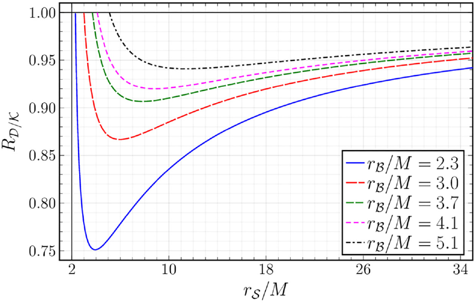
We present proper time ratios R_𝒟/𝒦: = Δ_τ𝒟/Δ_τ𝒦 in terms of r_𝒮/M in Fig. 6, for different values of r_B.

Figure 6
Proper time ratio R_𝒟/𝒦:= Δ_τ𝒟/Δ_τ𝒦 versus the start radius r_𝒮/M = r_𝒜/M = r_𝒦/M for distinct values of the bouncing radius r_ℬ/M.

We note that

• for any r_𝒮 ≥ r_ℬ, we have R_𝒟/𝒦 ≤ 1. Indeed, this is expected by our qualitative argument presented at the previous section. The observer 𝒟 is a 𝒴-type observer going into the fountain of youth region, therefore returning younger than the static observer 𝒦.

• for any 2M < r_ℬ ≤ r_𝒮, there is a radius r_s, corresponding to a minimum of R_𝒟/𝒦.

5.3. Observers 𝒟 and 𝒰

Let us suppose that at an event 𝒮, at the radius r = r_𝒮 an observer 𝒟 is released downward and an observer 𝒰 is vertically launched upward (cf. Fig. 4). To ensure that 𝒟 and 𝒰 meet again at the same event 𝒮 at r = r_𝒮, observer 𝒟 must be bounced, at a radius r = r_ℬ, and we ought to select appropriate combinations for the values of the parameters r_S, r_B and r_H, such that the round trip coordinate times satisfy Δt_𝒰 = Δt_𝒟 [cf. (40a) and (48)]. The proper time ratio R_𝒟/𝒰: = Δ_τ𝒟/Δ_τ𝒰 is shown in Fig. 7.

Figure 7
Proper time ratio R_𝒟/𝒰: = Δ_τ𝒟/Δ_τ𝒰 versus the bounce radius r_ℬ/M for distinct values of the start radius r_𝒮/M = r_𝒜/M.

5.4. Observers 𝒞 and 𝒦

Now we consider a circular geodesic observer 𝒞 at the radius of a comoving static Killing observer 𝒦 (cf. Fig. 4). The corresponding elapsed proper time for 𝒦 is given by

(49) $$\mathrm{\Delta }{\tau }_{{𝒦}_{𝒮\to 𝒜}}(M,r_{𝒞})=\sqrt{1-\frac{2M}{r_{𝒞}}}\mathrm{\Delta }{t}_{{𝒞}_{𝒮\to 𝒜}}(M,r_{𝒞}).$$

Using (37), we now find the ratio

(50) $$R_{𝒞/𝒦}(M,r_{𝒞}):=\frac{\mathrm{\Delta }{\tau }_{{𝒞}_{𝒮\to 𝒜}}(M,r_{𝒞})}{\mathrm{\Delta }{\tau }_{{𝒦}_{𝒮\to 𝒜}}(M,r_{𝒞})}=\sqrt{\frac{1-3M/r_{𝒞}}{1-2M/r_{𝒞}}}<1.$$

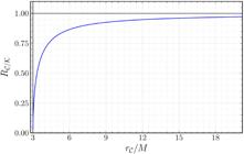
Therefore, observer 𝒞 always returns younger than 𝒦, i.e., the circular geodesic observer ages less than the static accelerated one. The qualitative result is also expected by the argument presented at the previous section – the fountain of youth is a cylindrical crown (in spacetime) or spherical crown (in space) that is closed in the exterior surface, so that 𝒞 is a 𝒴-type observer. The behavior of the ratio R_𝒞/𝒦 in terms of r_𝒞/M is shown in Fig. 8.

Figure 8
Proper time ratio R_𝒞/𝒦:= Δτ_𝒞/Δτ_𝒦 versus the circular radius r_𝒞/M = r_𝒦/M = r_𝒮/M = r_𝒜/M.

5.5. Observers 𝒰 and 𝒞

Let us consider now an observer 𝒞 in a circular geodesic orbit. Starting from a common event 𝒮 another observer 𝒰 is launched radially upwards in such a way that 𝒞 and 𝒰 meet again exactly at the event 𝒜 corresponding to a complete orbit (cf. Fig. 4).

To ensure that 𝒞 and 𝒰 meet again at the end of their trips, we need to adjust r_C and r_H accordingly, so that the elapsed coordinate times for the round trips of 𝒞 and 𝒰 coincide. The coordinate time associated to one complete orbit of 𝒞 is given, according to (36) by

(51) $$\mathrm{\Delta }{t}_{{𝒞}_{𝒮\to 𝒜}}(M,r_{𝒞})=2\pi \sqrt{\frac{r_{𝒞}^3}{M}},$$

and the corresponding coordinate time for 𝒰 to go up and return is, according to (40a), given by

(52) $$\begin{array}{l}\mathrm{\Delta }{t}_{{𝒰}_{𝒮\to 𝒜}}(M,r_{\mathscr{H}},r_{𝒮})\\ \mathrm{}=2E_{\mathscr{H}}\sqrt{{\displaystyle \frac{r_{\mathscr{H}}^3}{2M}}}{F}_1({\eta }_{𝒮},E_{\mathscr{H}})+4M{F}_2({\eta }_{𝒮},{\eta }_h).\end{array}$$

where F₁ and F₂ are given by (29), r_𝒞 = r_𝒮, $E_{\mathscr{H}}=\sqrt{1-2M/r_{\mathscr{H}}}$, η_h = 2 arcsin ⁡E_ℋ and η_𝒮 = arccos⁡(2r_𝒮/r_ℋ−1). Let us find values for r_C and r_H such that

(53) $$\mathrm{\Delta }{t}_{{𝒞}_{𝒮\to 𝒜}}(M,r_{𝒞})=\mathrm{\Delta }{t}_{{𝒰}_{𝒮\to 𝒜}}(M,r_{\mathscr{H}},r_{𝒞}),$$

The proper time of the observer 𝒰 is given by [cf. (39a)]

(54) $$\mathrm{\Delta }{\tau }_{{𝒰}_{𝒮\to 𝒜}}(M,r_{𝒮},r_{\mathscr{H}})=\sqrt{\frac{r_{\mathscr{H}}^3}{2M}}({\eta }_{𝒮}+\sin {\eta }_{𝒮}),$$

where r_𝒮 = r_𝒞, and Δτ𝒞 is given by (37), where E_𝒞 is given by (33).

The behavior of R_𝒰/𝒞: = Δ_τ𝒰/Δ_τ𝒞 in terms of r_C is shown in Fig. 9 In other words, observer 𝒞 returns younger than 𝒰, as expected. When r_𝒞 → 3M, Δ_τ𝒰/Δ_τ𝒞 → ∞.

Figure 9
Proper time ratio R_𝒰/𝒞:= Δ_τ𝒰/Δ_τ𝒞 versus the circular radius r_𝒞/M = r_𝒮/M = r_𝒜/M.

5.6. Observers 𝒟 and 𝒞

Finally, let us find the respective elapsed proper times of an observer 𝒞 in a circular orbit, at r = r_𝒞 > 3M, and an observer 𝒟 falling downward radially from r = r_𝒞, bouncing in a perfectly elastic way at r = r_ℬ ∈ (2M, r𝒞) and returning to r = r_𝒞 to meet 𝒞 (cf. Fig. 4). To ensure that 𝒞 and 𝒟 meet again at the end of their trips, we need, analogously to what we did in the previous subsection, to adjust r_C and r_B accordingly so that the elapsed coordinate times for the round trips of 𝒞 and 𝒟 coincide. The coordinate time associated to one complete orbit of 𝒞 is given, according to (36), by

(55) $$\mathrm{\Delta }{t}_{{𝒞}_{𝒮\to 𝒜}}(M,r_{𝒞})=2\pi \sqrt{\frac{r_{𝒞}^3}{M}},$$

and the corresponding coordinate time for 𝒟 to go down, bounce and return is, according to (48), given by

(56) $$\begin{array}{l}\mathrm{\Delta }{t}_{{𝒟}_{𝒮\to 𝒜}}(M,r_{𝒮},r_{ℬ})\\ \mathrm{}=\left[2E_{𝒮}\sqrt{{\displaystyle \frac{r_{𝒞}^3}{2M}}}{F}_1({\eta }_{ℬ},E_{𝒮})+4M{F}_2({\eta }_{ℬ},{\eta }_h)\right],\end{array}$$

where F₁ and F₂ are given by (29), $E_{𝒮}=\sqrt{1-2M/r_{𝒞}}$, η_h = 2 arcsin ⁡E𝒮 and η_ℬ = arccos⁡(2r_ℬ/r_𝒞−1).

Let us find values for r_B and r_C such that

(57) $$\mathrm{\Delta }{t}_{{𝒟}_{𝒮\to 𝒜}}(M,r_{𝒞},r_{ℬ})=\mathrm{\Delta }{t}_{{𝒞}_{𝒮\to 𝒜}}(M,r_{𝒞}).$$

Solving numerically the equation above shows that a pair of solutions (r_𝒞, r_ℬ) always exists, albeit for r_B very close to the horizon r_h = 2M. As r_C grows, r _ℬ → 2M, as shown in Fig. 10. The proper times of the observers 𝒞 and 𝒟 are given by (37) and (46) (with r_𝒮 = r_𝒞). In Fig. 11, we observe the surprising result that observer 𝒟 may return younger or older than 𝒞, depending on r_𝒞/M. For r_𝒞/M ≈ 3.21337 both observers are at the same age at the end of the journey. This reversal of differential aging is, however, to be expected since, as r_𝒞 → 3M, the circular geodesic 𝒞 becomes arbitrarily close to a null geodesic, causing its elapsed proper time to approach zero.

Figure 10
Bounce radius r_ℬ/M of twin 𝒟 versus circular radius r_𝒞/M of twin 𝒞, under the constraint of equal elapsed coordinate times, along twins 𝒟 and 𝒞.

Figure 11
Proper time ratio R_𝒟/𝒞:= Δ_τ𝒟/Δ_τ𝒞 versus the circular radius r_𝒞/M = r_𝒮/M = r_𝒜/M.

In contrast, it is worth mentioning that if we try, in the Newtonian case, to arrange the observers 𝒞 and 𝒟 to reunite after an exact orbital period of 𝒞 and a bounce of 𝒟, this turns out to be impossible.

This example shows that the “fountain of youth” argument holds only if the observer compared with 𝒴 is the static observer 𝒦 – for a general observer outside the fountain of youth, the observer going inside it may return older. One could argue that 𝒞 is also inside the fountain of youth region, as it is closed in the exterior surface. However, as 𝒞 is at the boundary, we may add measure zero radial curves that throw it away from the fountain of youth without affecting the total proper time elapsed.

6. Universal Differential Aging and Doppler Effect?

A connection between the differential aging and the Doppler effect often appears in the literature [²⁸, ²⁹]. We would like to take the opportunity here to make some remarks on this issue, which is also connected to the observation regarding the measuring of times by observers, on page 1. In fact, it will turn out to be expedient to distinguish between two kinds of Doppler effect, in a generic curved spacetime.

The Doppler effect between two instantaneous observers [cf. Fig. 12, panel (a)] involves the comparison of the wavelengths measured by exactly two instantaneous observers, $(ℰ,u_{ℰ}^{\alpha })$ and $(ℛ,u_{ℛ}^{\alpha })$, defined at an emission event ℰ and a reception event ℛ, connected by a null geodesic 𝒩, in an arbitrary spacetime (ℳ, g_αβ). The Doppler shift is defined by

Figure 12
(a) Doppler effect between instantaneous observers; (b) Doppler effect between observers, and (c) relationship between Doppler effect and differential aging.

(58) $$z[u_{ℰ}^{\alpha }\to u_{ℛ}^{\alpha }]\text{:=}{\displaystyle \frac{\mathrm{\Delta }\lambda }{{\lambda }_{ℰ}}}\text{:=}{\displaystyle \frac{{\lambda }_{ℛ}-{\lambda }_{ℰ}}{{\lambda }_{ℰ}}},$$

or, equivalently,

(59) $$1+z[u_{ℰ}^{\alpha }\to u_{ℛ}^{\alpha }]=\frac{{\lambda }_{ℛ}}{{\lambda }_{ℰ}}=\frac{{\left(k^{\alpha }{u}_{\alpha }\right)|}_{ℛ}}{{\left(k^{\beta }{u}_{\beta }\right)|}_{ℰ}}.$$

If we change the instantaneous observers: $(ℰ,u_{ℰ}^{\alpha })\mapsto (ℰ,{\overline{u}}_{ℰ}^{\alpha })$, $(ℛ,u_{ℛ}^{\alpha })\mapsto (ℛ,{\overline{u}}_{ℛ}^{\alpha })$, the Doppler shift changes as

(60) $$1+z[{\overline{u}}_{ℰ}^{\alpha }\to {\overline{u}}_{ℛ}^{\alpha }]=\mathrm{}(1+z[{\overline{u}}_{ℰ}^{\alpha }\to u_{ℰ}^{\alpha }])(1+z[u_{ℰ}^{\alpha }\to u_{ℛ}^{\alpha }])\times (1+z[u_{ℛ}^{\alpha }\to {\overline{u}}_{ℛ}^{\alpha }]),$$

or in a lighter (but not so explicit) notation,

(61) $$1+{\overline{z}}_{ℰ\to ℛ}=\left(1+z_{\text{loc},ℰ}\right)\left(1+z_{ℰ\to ℛ}\right)\left(1+z_{\text{loc},ℛ}\right).$$

Some observations are in order: (i) in a general spacetime the global Doppler shifts (${\overline{z}}_{ℰ\to ℛ}$ and z_{ℰ → ℛ}) cannot be unambiguously conceived as arising from two objective, absolute contributions: one kinematic and another gravitational (or cosmological). Only when there is a class of privileged instantaneous observers (arising, e.g., from some isometry, such as in Schwarzschild, Kerr or Robertson-Walker spacetimes) does such a decomposition make sense; (ii) in this pure context, one cannot relate the Doppler effect and the differential aging, since we do not have meeting observers at issue.

Panel (b) of Fig. 12, in contrast, illustrates the Doppler effect between two observers, 𝒪₁ and 𝒪₂. Here we are again unable to directly relate this situation to the differential aging since, although there are now indeed two observers, they do not meet.

Only in the situation illustrated in Fig. 12, panel (c), where the observers now do meet, does it make sense to speak about both the redshift between instantaneous observers along 𝒪₁ and 𝒪₂ and their differential aging. Granting that, we might then inquire whether there is a universal relationship, in a generic spacetime, between the differential aging and the Doppler shift.

For the prototypical case of the differential aging in Minkowski spacetime shown in Fig. 13, it is apparent, from the monitoring of the Doppler shift between the inertial observer 𝒪₁ and the piecewise inertial observer ${𝒪}_2={𝒪}_2^{\prime }\cup {𝒪}_2^{″}$, that 𝒪₂ gets younger than 𝒪₁.

Figure 13
Prototypical differential aging scenario in Minkowski spacetime. 𝒪₁ is a differentiable geodesic observer and observer ${𝒪}_2={𝒪}_2^{\prime }\cup {𝒪}_2^{″}$ is a piecewise differentiable geodesic observer, constituted by two geodesic observers ${𝒪}_2^{\prime }$ and ${𝒪}_2^{″}$, with a common bounce (or break) event ℬ, which have the same (3-)speed relative to 𝒪₁, but in opposite directions. Thus there is a single null geodesic _𝒩, emitted by 𝒪₁, at event _ℰ, which connects to the reception event ℛ₁:= ℬ, at 𝒪₂.

The proper time τ_{O1S →E1} elapsed along 𝒪₁, from 𝒮 to ℰ₁, is shorter than the proper time τO_2S→R1 elapsed along 𝒪₂, from 𝒮 to ℛ₁, because of their redshift. Now, by reciprocity, in the approaching stage, there is the same ratio of proper times but now giving rise to a blueshift. Thus the proper time τ_O1E1→A elapsed along 𝒪₁, from _ℰ to 𝒜 is longer than the proper time τ_O2R1→A elapsed along 𝒪₂, from ℛ₁ to 𝒜, by the very same ratio. Moreover, by the symmetry of this prototypical problem, we have

(62) $${\tau }_{𝒪_2{}_{𝒮\to {ℛ}_1}}={\tau }_{𝒪_2{}_{{ℛ}_1\to 𝒜}}=x$$

On the other hand, we may write:

(63) $$\begin{array}{c}\hfill {\tau }_{𝒪_1{}_{𝒮\to {ℰ}_1}}=K{\tau }_{𝒪_2{}_{𝒮\to {ℛ}_1}}=Kx;\\ \hfill {\tau }_{𝒪_1{}_{{ℰ}_1\to 𝒜}}=\frac{1}{K}{\tau }_{𝒪_2{}_{{ℛ}_1\to 𝒜}}=\frac{x}{K}\end{array}$$

where 0 < K < 1. Finally, we get:

(64) $$\begin{array}{l}{\tau }_{𝒪_1{}_{𝒮\to 𝒜}}={\tau }_{𝒪_1{}_{𝒮\to {ℰ}_1}}+{\tau }_{𝒪_1{}_{{ℰ}_1\to 𝒜}}\\ =\left(K+{\displaystyle \frac{1}{K}}\right)x>2x={\tau }_{𝒪_2{}_{𝒮\to 𝒜}}.\end{array}$$

Thus, we see that, directly based on a Doppler shift argument, the twin 𝒪₁ indeed gets older than the twin 𝒪₂. Of course, this result is much more easily obtained via the expression for the interval in pseudo-Cartesian coordinates adapted to the inertial observer 𝒪₁.

However, in a generic spacetime, and even in Schwarzschild spacetime, things are subtler, as we have remarked in the counterexamples of Sec. 5. In fact, using Doppler shift formulas for observers 𝒦, and 𝒰, it can be shown (e.g., [³⁰]) that we can have blueshift and redshift at different stages of the journey. Intuitively, there will always be an initial stage in which the twins measure a redshift and then eventually a final stage in which they measure a blueshift, for after all they are initially “receding” and then eventually “approaching”. However, in a curved spacetime context, in contrast to that prototypical Minkowski spacetime case, we no longer have such a high symmetry of the observers and a vanishing curvature. Of course, from Eqs. (59) and (61), we can always choose instantaneous observers, at emission and reception events, which are parallel transported (along the connecting null geodesic) and this implies the corresponding global Doppler shift $z_{ℰ\to ℛ}$ vanishes; one then only needs to take into account the local (pointwise) Doppler shifts at emission, z_loc,E, and reception, z_loc,R, via usual Lorentz boosts [cf. Fig. 12, panel (a)]. This does not provide much insight because the final global Doppler shift ${\overline{z}}_{ℰ\to ℛ}$ is determined by the aforementioned boosts, which camouflage the curvature/metric via the parallel transportation.

We claim the bottom line is that, in a generic, arbitrary spacetime, to compare the elapsed proper times along two arbitrary observers, there is no easy replacement for the calculation of the corresponding line integrals; in some very specific cases, one may resort to local theorems [e.g. [²²]].

7. Discussion

We have systematically studied the differential aging in a vacuum Schwarzschild spacetime, deriving the proper time intervals for four convenient observers (“twins”): a static Killing one (𝒮), two smooth geodesic ones (𝒰 and 𝒞) and a sectionally geodesic one (𝒟). We plotted all six independent corresponding proper time ratios, and we now present a summary of the qualitative results in Table 2.

TABLE 2
Twins (𝒪₁,𝒪₂) and corresponding proper time ratio R_𝒪1/𝒪₂:= Δτ_𝒪1/Δτ_𝒪2 (cf. the cited Figure for a relevant plot of R_𝒪1/𝒪₂×r_*/M, where r_* is a relevant radius which characterizes the arrangement of the twins).

Twins [(𝒪1,𝒪2)]	Proper time ratio R𝒪1,𝒪2 [Fig.]
(𝒰,𝒦)	≥1 [5]
(𝒦,𝒟)	≥1 [6]
(𝒰,𝒟)	≥1 [7]
(𝒰,𝒞)	≥1 [9]
(𝒞,𝒦)	≤1 [8]
(𝒞,𝒟)	⋚1 [11]

The key takeaway points we want to stress are conveniently summarized in Table 2, which suggests, by means of examples in its first four rows, for the twins (𝒰,𝒦), (𝒦,𝒟) (𝒰,𝒟) and (𝒰,𝒞), that the twin that travels closer to the matter source indeed gets younger than the one which stays further away. However this same table, in its last two rows, provides two enlightening and silver-bullet counterexamples to two diehard myths: (i) for the twins (𝒟,𝒞) there is a range of initial conditions such that the twin 𝒟, which is always closer to the source, returns older than the twin 𝒞, which always remains further away; (ii) the geodesic twin 𝒞 gets younger than the accelerated twin 𝒦, despite being always at the same radius, and thus somehow subjected to the “same” gravitational field. It is in fact true that the counterexample we found here for observer 𝒞 is not very realistic, inasmuch as its radius has to be close to 3M, i.e., inside the interval 3M < r < 6M, being therefore an unstable orbit. Moreover, if we choose, at a certain event of the curve 𝒞, the associated instantaneous observer${\overline{u}}^{\alpha }$, given by [cf. (36) and (37)]

(65) $${\overline{u}}^{\alpha }={\frac{d{x}^{\alpha }}{d\tau }|}_{𝒞},$$

and take the Killing instantaneous observer u^α defined, at the same event, by

(66) $$u^{\alpha }=\frac{1}{\sqrt{1-2M/r}}{\delta }_0^{\alpha },$$

we can calculate the relative speed v between them via

(67) $$\gamma (v):=\frac{1}{\sqrt{1-v^2}}=-{\overline{u}}^{\alpha }{u}_{\alpha }.$$

Indeed, this speed is very close to the speed of light, as we now show. From (65) to (67):

(68) $$\gamma (v)={\sqrt{-g_{00}}\frac{d{x}^0}{d\tau }|}_{𝒞}={\sqrt{1-\frac{2M}{r_{𝒞}}}\frac{dt}{d\tau }|}_{𝒞}.$$

Using (37) and (33), we also have:

(69) $${\frac{dt}{d\tau }|}_{𝒞}=\frac{E_{𝒞}}{1-2M/r_{𝒞}}=\frac{1}{\sqrt{1-3M/r_{𝒞}}}.$$

Comparing the above expressions:

(70) $$\frac{1}{\sqrt{1-v^2}}=\frac{\sqrt{1-2M/r_{𝒞}}}{\sqrt{1-3M/r_{𝒞}}}\mathit{}⟹\mathit{}v=\sqrt{\frac{M}{r_{𝒞}-2M}}.$$

Setting the radius r_𝒞 ≈ 3.21337M, where both observers have the same age (cf. Subsec. 5.6), the corresponding relative speed turns out to be v ≈ 0.90783. Therefore, in order for the observer 𝒟 to return older than the observer 𝒞, v > 0.90783. This is expected since r = 3M corresponds to the innermost unstable circular null geodesic.

The deceptive claim of time running slower when we are closer to the mass source is also recurrent in the problem of the Doppler effect. We saw in Sec. 6 that the usual problem of the Doppler effect is in principle different from the issue of the differential aging. We may draw a correspondence between them only when the observers of the former meet in two different events.

As we have seen, even in this situation, the conclusions concerning the aging of observers are not immediate – in the problem described at the end of Sec. 6, we made strong use of symmetries both of the Minkowski metric and of the observers, which may be absent in more general situations. In fact, even in the still highly symmetric Schwarzschild case, for instance, among observers 𝒰 and 𝒦, the relation between the Doppler shift and differential aging is not clear.

A natural follow-up to this work would be extending this analysis to other observers still in the vacuum Schwarzschild spacetime [³¹], or to the region inside the vacuum Schwarzschild event horizon or to other spacetimes (such as has already been done for, e.g., Kerr [³²] and de Sitter spacetimes [³³]).

We have created a Github repository [³⁴], where the reader may find interactive Python notebooks to illustrate the ratio of proper times for the distinct pairs of observers. This repository also provides a glossary [¹¹] containing relevant terms from the terminology used in this paper.

References

• ^[1] K. Thorne, The science of Interstellar (W. W. Norton & Company, New York, 2014).
• ^[2] B. O’Neill, The geometry of Kerr black holes (A.K. Peters, Wellesley, 1995).
• ^[3] H. Stephani, Relativity: An introduction to special and general relativity (Cambridge University Press, Cambridge, 2004), 3 ed.
• ^[4] E.F. Taylor and J.A. Wheeler, Exploring black holes: Introduction to general relativity (Addison Wesley Longman, San Francisco, 2000).
• ^[5] M. Gleiser, The dancing universe: From creation myths to the Big Bang (University Press of New England, Lebanon, 2005).
• ^[6] L. Rezzolla, The irresistible attraction of gravity: A journey to discover black holes (Cambridge University Press, Cambridge, 2023).
• ^[7] C. Rovelli, The order of time (Riverhead Books, New York, 2018).
• ^[8] J. Ehlers, in: The physicist’s conception of nature , edited by J. Mehra (D. Reidel Publishing Company, Dordrecht, 1973).
• ^[9] J. Earman, World enough and space-time (MIT Press, Cambridge, 1989).
• ^[10] R. Penrose, The road to realtiy (Vintage Books, New York, 2007).
• ^[11] T.A.A. Camara, P.S. Lemos, M.O. Calvão and F.D. Sasse, https://github.com/fernandodeeke/Twin_Paradox/blob/main/glossary.pdf
  » https://github.com/fernandodeeke/Twin_Paradox/blob/main/glossary.pdf
• ^[12] R.K. Sachs and H.H. Wu, General relativity for mathematicians (Springer, New York, 1977).
• ^[13] W. Rindler, Introduction to special relativity (Oxford University Press, Oxford, 1991), 2 ed.
• ^[14] L. Parker and L.O. Pimentel, Phys. Rev. D 25, 3180 (1982).
• ^[15] C.H. Brans and D.R. Stewart, Phys. Rev. D 8, 1662 (1973).
• ^[16] T. Dray, Am. J. Phys. 58, 822 (1990).
• ^[17] J.D. Barrow and J. Levin, Phys. Rev. A 63, 044104 (2001).
• ^[18] J.P. Uzan, J.P. Luminet, R. Lehoucq and P. Peter, Eur. J. Phys. 23, 277 (2002).
• ^[19] L.M. Sokołowski, Gen. Relativ. Gravit. 44, 1267 (2012).
• ^[20] S.W. Hawking and G.F.R. Ellis, The large scale structure of space-time (Cambridge University Press, Cambridge, 1973).
• ^[21] R.M. Wald, General relativity (The University of Chicago Press, Chicago, 1984).
• ^[22] L.M. Sokołowski, Demonstratio Math. 50, 56 (2017).
• ^[23] S. Chandrasekhar, The mathematical theory of black holes (Oxford University Press, Oxford, 1983).
• ^[24] C.W. Misner, K.S. Thorne and J.A. Wheeler, Gravitation (W.H. Freeman and Company, San Francisco, 1973).
• ^[25] J.B. Hartle, Gravity: An introduction ot Einstein’s general relativity (Addison Wesley, San Francisco, 2003).
• ^[26] S.M. Carroll, Spacetime and geometry: An introduction to general relativity (Addison Wesley, San Francisco, 2004).
• ^[27] Ø. Grøn and S. Braeck, Eur. Phys. J. Plus 126, 79 (2011).
• ^[28] W. Rindler, Relativity: Special, general, and cosmological (Oxford University Press, Oxford, 2006), 2 ed.
• ^[29] B. Schutz, A First Course in General Relativity (Cambridge University Press, Cambridge, 2022), 3 ed.
• ^[30] M. Kasai, arXiv:2302.11146 (2023).
• ^[31] K.K.H. Fung, H.A. Clark, G.F. Lewis and X. Wu, Eur. J. Phys. 37, 055602 (2016).
• ^[32] F.L. Markley, Am. J. Phys. 41, 1246 (1973).
• ^[33] S. Boblest, T. Müller and G. Wunner, Eur. J. Phys 32, 1117 (2011).
• ^[34] T.A.A. Camara, P.S. Lemos, M.O. Calvão and F.D. Sasse, https://github.com/fernandodeeke/Twin_Paradox
  » https://github.com/fernandodeeke/Twin_Paradox

• 1
  In fact, the geometrical structure of the classical (nonrelativistic) spacetimes is, somewhat surprisingly, more complex than the Lorentzian relativistic ones; cf. e.g. [⁸, ⁹, ¹⁰].
• 2
  Some italicized expressions are defined in a glossary at github [¹¹].
• 3
  If, in a given spacetime endowed with an isometry, there exist two observers connected by such an isometry which intersect at two events, then their elapsed proper times between such events must be equal, and thus there is no relative aging at all.
• 4
  Beware: in the literature, it is common to refer to the whole vacuum Schwarzschild spacetime also as the exterior Schwarzschild spacetime (in contrast to the interior, matter-filled one).
• 5
  Technically, we have two charts: one for 0 < r < 2M, and another for 2M < r < ∞.

Edited by

• Editor-in-Chief:
  Marcello Ferreira https://orcid.org/0000-0003-4945-3169

Publication Dates

• Publication in this collection
  15 Sept 2025
• Date of issue
  2025

History

• Received
  15 Feb 2025
• Reviewed
  04 July 2025
• Accepted
  26 July 2025