Small oscillations study of a nonlinear circular oscillator

Abstract

We propose an experiment using the Arduino platform with MPU6050 accelerometer to obtain data from small oscillations of a circular rotating system which proved to be strongly nonlinear. The experimental setup uses a 3B-Scientific circular airflow bed as a structural basis for the experiment. We use the Lagrangian formalism to obtain the differential equation of the physical system, addressing the approximations that lead to the correct description of the potential energy involved. The proposed experiment is a good test to explore the non-linearity of ordinary differential equations in mechanical systems, besides being a topic of interest for engineering and physics courses.

Keywords:
Circular oscillator; nonlinear oscillations; MPU6050

1. Introduction

The harmonic oscillator is one of the fundamental tools for physical models [¹, ², ³]. Its study in different experimental setups and the theoretical underlying development has been the core of several canonical physical theories. The grasp of the relation between different types of energy involved is the key to the myriad of applications of such a system.

In the last century, many advances in microscopic models have derived from this well-known physical system, including technological impacts incommensurable with the development of Quantum Theory.

Since the first in-depth study of the simple harmonic oscillator by Christiaan Huygens in the 17th century, different configurations have been suggested as starting points for physical models. In particular, configurations in which dissipative forces act to extract energy from the system are of great interest due to realistic applications in Classical Mechanics [¹]. Furthermore, nonlinear terms in theoretical models appear recurrently, renewing interest in such systems [⁴,⁵,⁶].

Experimentally, some configurations involve inverted pendulum, spring-mass system with nonlinear spring, simple pendulum with variable mass or even nonlinear oscillations in electronic circuits. In this sense, we propose a mechanical configuration that considers the oscillations of a disc under the action of a linear spring fixed at a fixed point and another at a point tangent to the disc, as we will see schematically below.

In order to obtain the equations of motion, we will use the Lagrangian formalism, addressing the approximations that lead to a correct description of the potential energy involved [⁴]. The dissipative effect is added through the Rayleigh dissipation function incorporated into the theoretical discussion. This will lead us towards the generalized Euler-Lagrange equation associated with the experiment [⁴–⁶]. Next, we use the small oscillations approach to obtain system behaviors that fit the experimental data.

The experimental setup uses a 3B-Scientific circular airflow bed [⁷] with a Start/Stop push button as a structural basis for the experiment. The experimental acquisition data is performed through an Arduino IDE with a MPU6050 accelerometer [⁸]to measure the angular speed of the disc in the small oscillations regime. The Arduino platform has enabled the development of several experiments in physics laboratories, mainly due to the availability of increasingly accurate and affordable sensors [⁹, ¹⁰]. The proposed experiment is a good test to explore the nonlinearity of ordinary differential equations in mechanical systems, since this is a topic of interest for some engineering and physics courses. The nonlinear oscillator experiment can be effectively scaled across different educational levels. At the introductory undergraduate stage, it serves as a powerful qualitative demonstration to highlight the limitations of the idealized Simple Harmonic Oscillator model, showing students how real-world phenomena can be modeled from theory. For advanced undergraduates, the experiment transitions into a quantitative, hands-on laboratory experience where they apply their knowledge of differential equations to model the system, use advanced data acquisition and analysis techniques (such as FFT and phase-space plotting), and rigorously compare their empirical data to theoretical predictions, using different tools available with computer algorithms. At the graduate level, the same apparatus becomes a versatile platform for project-based research, allowing students to explore complex dynamics like bifurcations, routes to chaos, and synchronization, effectively using it as a model system for more advanced studies.

This paper is outlined as follows: in section 2, we present the proposed experimental setup. In section 3, we discuss the theoretical approach of the nonlinear circular oscillator. In section 4, we present the analysis of the experiment in light of the theoretical approach and the experimental data. Finally, in section 5, we present the conclusions and perspectives.

2. Experimental Setup

The experiment setup uses the 3B-Scientific rotary air bed system. The simplest version of this kit does not have any electronic sensors for measurement, data acquisition system based on a laser unit or anything similar. The number of experiments possibly performed is therefore underestimated. To get around this situation, you can use Arduino to set up other experiments with some good commercially available sensors. This is our objective when proposing an experiment using the Arduino platform with an MPU6050 accelerometer to obtain data from small oscillations of a rotating circular system that proved to be strongly nonlinear, as we will see later. As a starting point, we configure the 3B-Scientific rotary system by attaching a spring with k ≈ 10 N/m to the end of the bar using a small screw that serves as a fixing point; the other end is attached to a small laboratory clamp fixed to a vertical rod positioned at the base of the kit. This spring constant value may vary in the range 8-12 N/m, corresponding to ±20% of the reference value. Higher and smaller values were tested and resulted in friction between the disc and base, which will be addressed in the next section. To apply some tension to the spring, a rope is fixed at the same attachment point passing through the pulley positioned at the other end of the base support rod with support for small weights to which 30 g will be assigned. This assigned weight is important to activate the oscillator and keep friction well controlled, giving a longer duration to small oscillations. This first part of setup can be seen in Figure 1.

Figure 1
Experimental setup for the nonlinear oscillator.

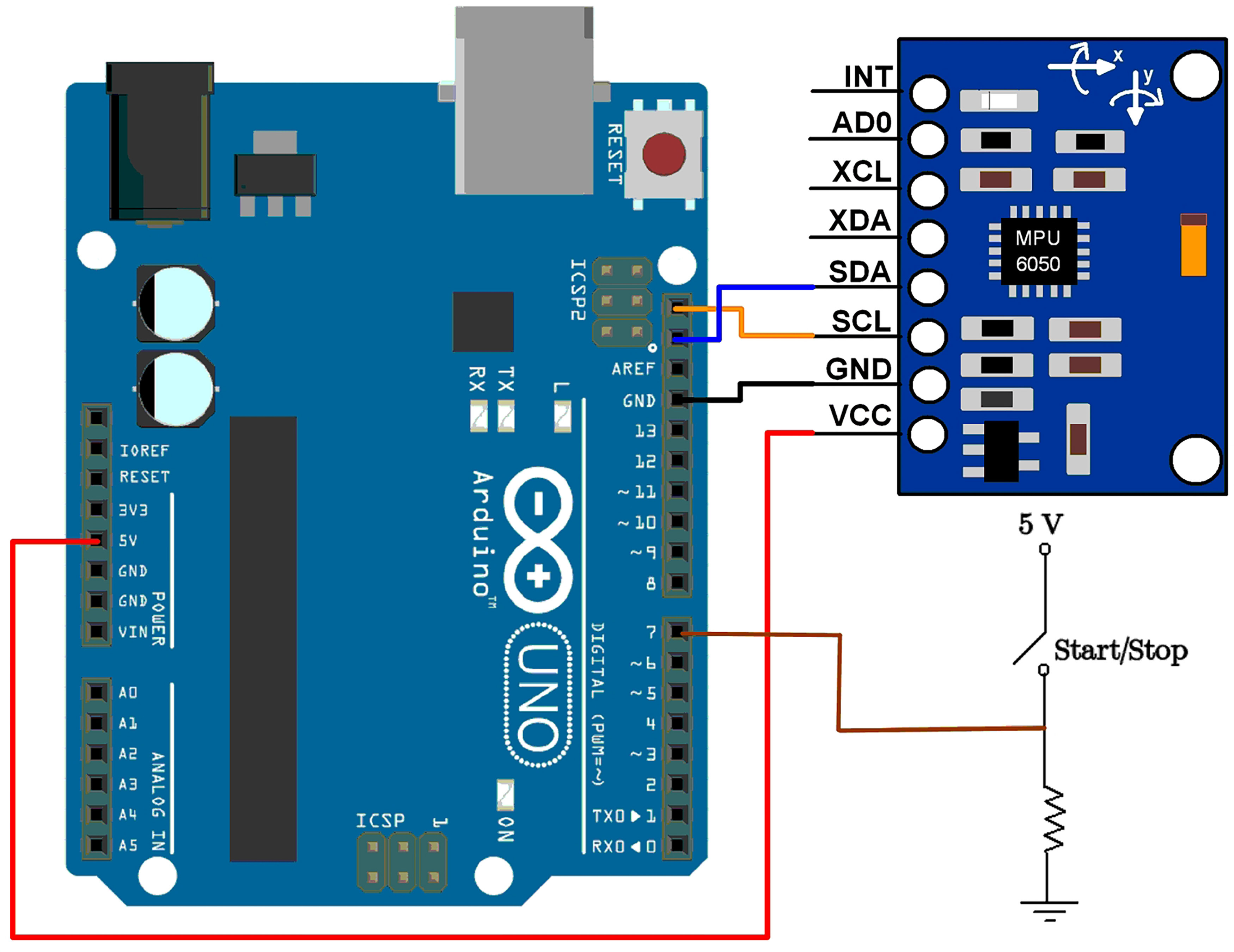
The Start/Stop module can also be visualized in Figure 1. It is a small plastic arm that attaches to a small switch and will be used to trigger the time via Arduino IDE programming, which will be available via supplemental material. In Figure 2 we show the MPU6050 positioned in the center of the disc through a small support. This can be done using a small plastic rod attached to a small plastic disc as a base, held together by a screw. In this kit, the center base of the disc on top of the pulleys is magnetic and will serve as a good adhesive. This is important because the MPU6050 will be connected to the Arduino via long wires to allow the freest possible movement of the spinning disc. It is necessary to assess whether the small oscillations are such that the wires do not interfere with them. To do this, you can make an initial data acquisition and plot the results, trying to observe any deformations at the beginning of the graph or simply try to guess the balance point of the MPU6050 base support by making a small oscillation without any measurements to check if the wires are loose. In Figure 5 we show the connections of the Start/Stop and the MPU6050 to the Arduino.

Figure 2
MPU6050 positioned on the disc.

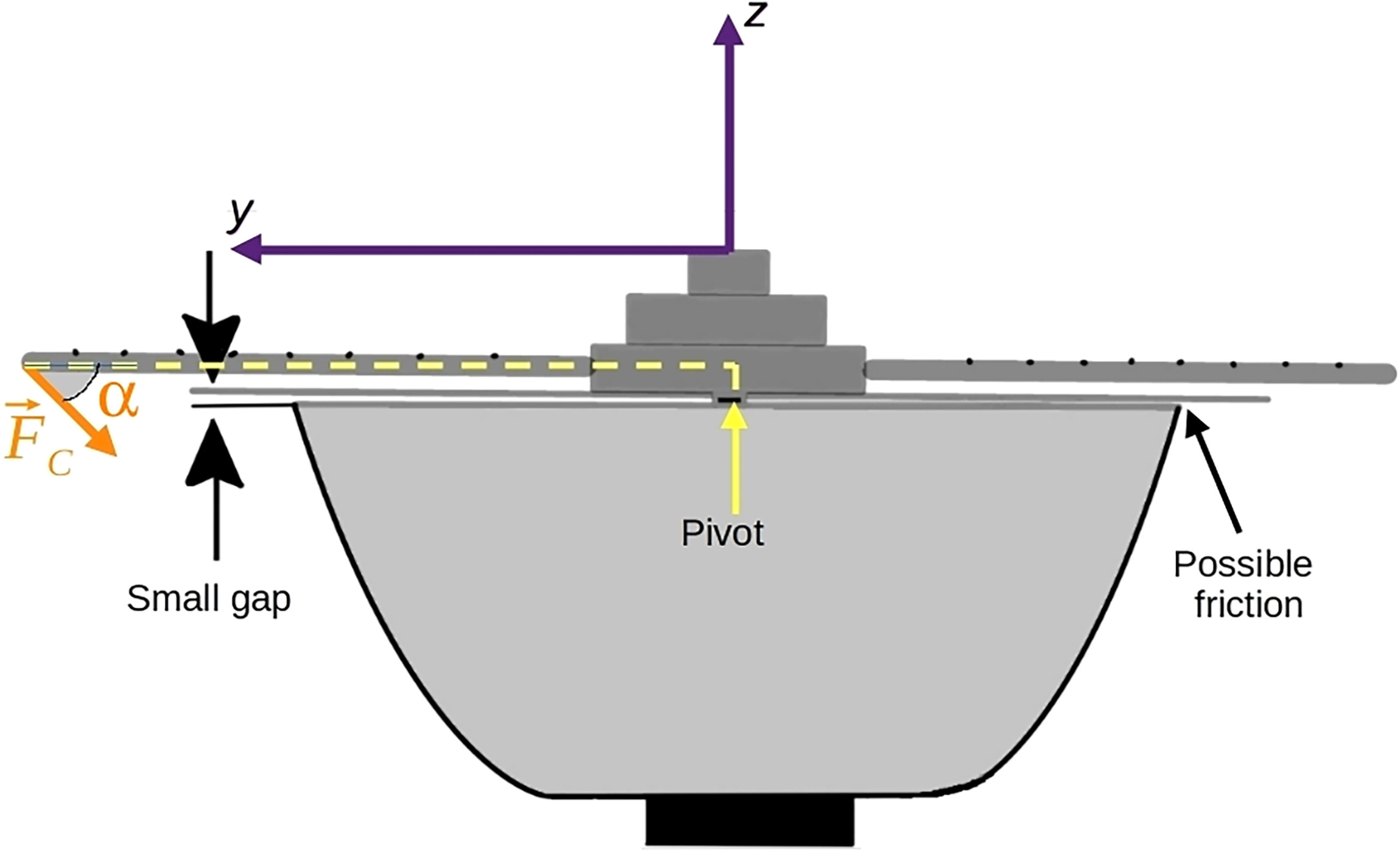
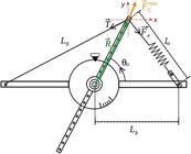
Now, let’s analyze the main forces involved. In Figure 3 we have a tension, $\overrightarrow{T}$, across the string and the elastic force, $\overrightarrow{F_e}$, applied by the spring at the same point on the bar. Let’s first illustrate the scenario in equilibrium, and apply Newton’s third law to the point of contact on the bar, creating a reaction contact force, ${\overrightarrow{F}}_C^{reac}$, to make the net force zero. The contact force, ${\overrightarrow{F}}_C$ due to the projection of $\overrightarrow{T}$ and $\overrightarrow{F_e}$ along the bar, generates a torque, pointing outwards the page, about the pivot point at the center of the disc that is coupled to the airflow bed as depicted in Figure 4. The pivot point is located at a small distance bellow the line of the bar, and any projection of contact force along the bar generates a torque that creates a small gap between the disc and the airflow bed base in the side of the contact point. As a result, the disc may touch the opposite side of the airflow bed, increasing frictional forces. To compensate for this, we adjust the hight of the pulley in the support base rod and the clamp attached to the spring so that a small angle, α < 10°, can be formed with the horizontal line, as can be seen in Figure 1. This arrangement creates a projection of the contact force, $\overrightarrow{F_c}$, that points downward, creating a torque compensation opposite to the torque of the projection of the contact force along the bar disc. When the disc is set in motion, the torque due to the net force takes over in the z direction and the harmonic motion is activated.

Figure 3
Diagrammatic top view scheme of the experimental setup in equilibrium.

Figure 4
Airflow bed with a side view.

Figure 5
Arduino configuration for MPU6050 and Start/Stop adapted from Ref. ⁸.

Finally, after these adjustments, we can proceed with data acquisition. The code in supplemental material Listing 1 uses some libraries that must be installed before data acquisition [⁸]. It is important to note that the Start/Stop must be in the position that holds the disc. After the program is loaded into the Arduino with the correct baud rate, a message should appear in the Arduino IDE’s serial monitor: “MPU6050 found!”, and “Temperature in Celsius:”. Now we can start the oscillations by rotating the disc at an angle ≲10°, causing tension in the spring and releasing the Start/Stop.

3. Theoretical Approach

The experimental parameters relevant to our analysis are shown in Figure 3. The geometry depends on bar half-length R, the spring’s initial length l₀, the rope’s initial length L₀, the distance L_b between the spring fixation point at the end of the kit base and the center of the disc, and, finally, the angle θ₀ is defined as the angle between the bar of the disc and the line of the support base due to the tension caused by the assigned mass of 30g to the system in equilibrium. If one applies the law of cosines.

(1) $$\begin{array}{l}{l}_0=\sqrt{R^2+L_b^2-2R{L}_b\cos {\theta }_0}\hfill \\ L_0=\sqrt{R^2+L_b^2+2R{L}_b\cos {\theta }_0}\hfill \end{array}$$

Consequently, the total mechanical potential energy is given by [⁴]

(2) $$\begin{array}{c}U(\theta )=\frac{k}{2}{\left(\sqrt{R^2+L_b^2-2R{L}_b\cos \theta }-l_0\right)}^2\\ +mg\left(\sqrt{R^2+L_b^2+2R{L}_b\cos \theta }-L_0\right)\end{array}$$

with k, m and g being the spring constant, the suspended mass and gravitational constant, respectively.

The geometric parameters in this experiment, (R, L_b, l₀, L₀, θ₀), cause the contribution of gravitational potential energy to be smaller than the elastic potential energy, such that only the elastic contribution to the total potential energy can be taken as a first approximation. There are two ways to see that: one is to plot the ratio of the two potential energies and the other is to expand around θ₀ and compare them term by term. However, we let to the reader to take this decision an we consider all contributions to the total potential energy. Since we are interested in small oscillations, we can expand around the equilibrium angle θ₀ to obtain.

$$U(\theta )=U_0+C_1\left(\theta -{\theta }_0\right)+\frac{C_2}{2}{\left(\theta -{\theta }_0\right)}^2+\frac{C_3}{6}{\left(\theta -{\theta }_0\right)}^3+\cdots$$

where U₀ = U(θ₀) = 0.

Defining β_g = mgRL_b/L₀, one can write the coefficients $C_n={\left[\frac{d^{n}U}{d{\theta }^n}\right]}_{{\theta }_0}$ as

(3) $$\begin{array}{l}{C}_1=-{\beta }_g\sin {\theta }_0\hfill \\ C_2=\frac{k{R}^2{L}_b^2}{l_0^2}{\sin }^2{\theta }_0-{\beta }_g\left(\cos {\theta }_0+\frac{{\beta }_g}{mg{L}_0}{\sin }^2{\theta }_0\right)\hfill \\ C_3={\beta }_g\sin {\theta }_0+\left(\frac{3k{R}^2{L}_b^2}{l_0^2}-\frac{3{\beta }_g^2}{mg{L}_0}\right)\sin {\theta }_0\cos {\theta }_0\hfill \\ -\left(\frac{3k{R}^3{L}_b^3}{l_0^4}+\frac{3{\beta }_g^3}{m^2{g}^2{L}_0^2}\right){\sin }^3{\theta }_0\hfill \\ ⋮\hfill \end{array}$$

Now, let’s define ϕ = θ − θ₀ and, as a first approximation, we will take the first two non-zero terms of the infinite series to get

(4) $$U(\phi )=C_1\varphi +\frac{C_2}{2}{\varphi }^2+\frac{C_3}{6}{\varphi }^3$$

This allows us to write the corresponding Lagrangian for the system as

(5) $$ℒ=\frac{1}{2}I{\dot{\varphi }}^2-U(\varphi )=\frac{1}{2}I{\dot{\varphi }}^2-C_1\varphi -\frac{C_2}{2}{\varphi }^2-\frac{C_3}{6}{\varphi }^3$$

where I is the moment of inertia of the system composed of disc with the the bar supplied by the manufacturer.

The equation of motion can be derived using the generalized Euler-Lagrange equation [⁴–⁶]

(6) $$\frac{d}{dt}\left(\frac{\partial ℒ}{\partial \dot{\varphi }}\right)-\frac{\partial ℒ}{\partial \varphi }={𝒬}_{\varphi }^{bar}$$

where ${𝒬}_{\varphi }^{bar}$ is the generalized external force acting on the bar disc.

In one dimension, the damping force on a spring-mass system can be calculated through the Rayleigh dissipation function $ℱ({\stackrel{.}{x}}^2)=b{\stackrel{.}{x}}^2$/2 to obtain the generalized force through $𝒬=-dℱ/d\stackrel{.}{x}=-b\stackrel{.}{x}$. In two dimensions, the generalized force can be depicted into radial and tangent components for a particle at a distance r from the origin. As discussed in the textbooks of Classical Mechanics [⁴–⁶], the tangential component of the generalized force is identified as a torque, which is ${𝒬}_{\varphi }^p=$(distance from the origin)(tangent force)$=r(-br\stackrel{.}{\varphi })=-b{r}^2\stackrel{.}{\varphi }$. Following this idea, we can consider the bar as small homogeneous slices, each one contributing with $d{𝒬}_{\varphi }^{bar}=-2b\stackrel{.}{\varphi }\text{sgn}(s)sds$ for the total generalized force, where s is the distance from the center of the disc and we have introduced the sgn(s) to take into account the sign of tangent speed in the antipodal distances with respect to the center of the disc. We can now calculate the net damping force through the bar disc by integrating in s ∈ [−R, R], resulting in ${𝒬}_{\varphi }^{bar}=-2b{R}^2\stackrel{.}{\varphi }$. In fact, the small oscillations together with the small amplitude of the angular speed corroborates this hypothesis and this relation fits well the experimental data as we will see in Section 4. The minus sign means a net force opposing circular motion with angular speed $\stackrel{.}{\varphi }$. Taking Eq. (5) into Eq. (6) we obtain

(7) $$I\ddot{\varphi }+C_1+C_2\varphi +\frac{C_3}{2}{\varphi }^2=-2b{R}^2\dot{\varphi }$$

Now we end up with a constant C₁ in the differential equation above. To circumvent this, we make a change of variable ϕ = φ + ϕ_eq, which defines a new equilibrium point, ϕ_eq. If we make this substitution into Eq. (7) we can rewrite it as

(8) $$\ddot{\phi }+\eta \dot{\phi }+{\omega }_0^2\phi +ϵ{\phi }^2=0$$

where η = 2bR²/I, ${\omega }_0^2=(C_2+C_3{\varphi }_{eq})/I$, ϵ = C₃/2I, and ϕ_eq is determined by the condition

(9) $$\begin{array}{l}\frac{C_3}{2}{\varphi }_{eq}^2+C_2{\varphi }_{eq}+C_1=0\hfill \\ {\varphi }_{eq}=-\frac{C_2}{C_3}\pm \sqrt{\frac{C_2^2}{C_3^2}-\frac{2C_1}{C_3}}\hfill \end{array}$$

This equation defines two possible equilibrium points: one stable and other unstable that we will disregard as explained in Section 4. η and ${\omega }_0^2$ are the physical quantities related to the time constant of the amplitude decay and the period of oscillations of the system, respectively. ϵ has dimension s⁻² and is responsible for the nonlinear term in equation. It is important to note that ϵ can assume relatively large values, which makes a perturbative treatment impossible. The only way out is to solve this differential equation using numerical technics as we will see in next section.

4. Results and Analysis

The acquisition data follows the experimental setup displayed in Figures 1–5, through the serial monitor furnished by the Arduino IDE software. It might be more advantageous to write a small Python program to get data directly from the Arduino serial port and save it to a file. It’s outside the scope of this work, but you can find code to do this on Arduino forums. We provide the code for acquiring data from Arduino in the supplemental Material in Listing 1. This code was adapted from a tutorial on the MPU6050 website [⁸]. Once loaded into the Arduino, the code causes the Arduino to monitor digital pin 7 for a change in state. This is the state of the Start/Stop button, which starts reading data from the MPU6050 when the state changes. After the code is transmitted, the message “MPU6050 FOUND!” will appear on the serial monitor followed by the local temperature. Now an offset angle ≲10° must be provided and Start/Stop released to generate all experimental data.

It is importante to empahsize the MPU6050 gives the angular speed in degrees per second(°/s). As can be seen in the manufacturer datasheet one must calibrate the MPU6050 depending on the specifications of the accelerometer and gyroscope ranges as well as the filter bandwidth that we chose ±8g, ±500°/s and 21 Hz, respectively. The manufacturer specifies a typical error about ±0.5°/s for this configuration without calibration, and can vary with temperature and time of data acquisition. For our purposes, the time of acquisition data is less than 15 seconds, which makes MPU6050 good for the measurements. We tested the calibration by measuring during 1 minute with MPU6050 over a stable surface. The average values of angular speed obtained for the axis of interest were 100 times lower than this value, which means it is already calibrated. To obtain the best possible experimental data, it is necessary to repeat the measurements several times, as the wires connected to the MPU6050 can affect the movement and some settling before acquisition data is needed. It is important to emphasize that an initial amplitude greater than 10° should not be provided, or the spring may lose tension during part of the motion, affecting the measurements. Another undesirable effect can be the support slipping from the MPU6050 base. This can be easily identified by plotting the data and looking for deformations at the beginning of the acquisition data as we mentioned before.

Now, we need some analytical expression from theory to optimize parameters to fit the experimental data. Unfortunately, an analytical solution of Eq. (8) is not available. One way out is to provide a numerical integrator that does the job, giving us the optimized set of parameters of Eq. (8) that best fit the experimental data. In Python we have the SciPy library with several tools for this task.

In the supplemental material Listing 2, we provide a Python code that uses the SciPy library to solve the ODE suggested in Eq. (8), with the set of parameters (φ₀, η, ω₀, ϵ) to be determined inside a given range. This is a type of reverse problem that SciPy handles seamlessly, via the built-in SciPy.optimize library. The integrator uses SciPy’s built-in library to integrate ODEs with initial value problems, via SciPy.integrate. The file with data should be named “exp_data.txt”, formatted so that the data is separated by a single space, for simplicity. Firstly, to employ Eq. (8) one must convert the experimental data from °/s to rad/s. To this end, we introduce in line 10 of the code the conversion factor deg_rad (= π/180) that will be used to convert the experimental data in line 15. The first refers to an interval estimate for the initial value of φ, which was defined such that 5°≲φ₀≲12°, converted to radians. The others are related to η, ω₀, and ϵ, respectively. The manufacturer provides the value of I = 0.0009 kg.m² for the disc with the coupled bar moment of inertia.

To get an idea about these intervals, one should use Eq. (3) as a starting point. As illustrated in Figure 3, it is possible to measure the values of R, L_b, L₀, and l₀. These values were measured in our setup with a ruler, resulting in the values R = 21.00 ± 0.05 cm, L_b = 24.00 ± 0.05 cm, L₀ = 38.55 ± 0.05 cm, and l₀ = 26.00 ± 0.05 cm. The spring constant, k = 9.7 ± 0.5 N/m, was measured with a set of precision weights assigned to the spring with the respective deformations and plotted to obtain its best value through the least squares fitting method. As a result, one can use Eqs. (1) and (3) to calculate the values C₁/I = −40.2 ± 0.1 s⁻², C₂/I = 333 ± 22 s⁻², C₃/I = −355 ± 22 s⁻², giving ϵ = C₃/2I = −177 ± 11 s⁻², and using these values into Eq. (9) one gets ${\varphi }_{eq}^{(1)}=1.74\pm 0.16$ rad, and ${\varphi }_{eq}^{(2)}=0.13\pm 0.16$ rad. In this case, ${\varphi }_{eq}^{(1)}$ is the unstable value and, consequently, we take ${\varphi }_{eq}^{(2)}$, which leads to the stable solution with ω₀=$\sqrt{C_2/I+(C_3/I)*{\varphi }_{eq}^{(2)}}$=17 ± 2 rad/s.

The intervals to perform the adjustment are chosen to have these values between their limits. The possible range for η can be defined by taking as a starting point the value obtained by plotting the peaks of the experimental data and fit a function $\stackrel{.}{\phi }(t)={\stackrel{.}{\phi }}_0\exp (-\frac{\eta }{2}t)$ at the beginning of the measurements, i.e., to the first half of the measurement time, disregarding the other half with any least-squares algorithm. In our case, we obtained ${\stackrel{.}{\phi }}_0=3.93\pm 0.04$(×10⁻²)rad/s and η = 0.520 ± 0.002 s⁻¹. The Arduino code in Listing 1 prints time for each 0.05 s. As a good estimate for φ₀, one can calculate the product of $\stackrel{.}{\phi }$ by 0.05 s, which gives φ₀ = 0.196 ± 0.002(×10⁻²)rad. Some adjustments may be necessary if one or more of these optimized variables in the program output vary too close to the bounds of the limits. This will result in an inadequate adjustment of the integrator to the experimental data. As a consequence, the ranges for (φ₀, η, ω₀, ϵ) chosen as an input to the program were such as φ₀ ∈ [0.0014,0.04] rad, η ∈ [0.35,0.75] s⁻¹, ω₀ ∈ [10,20] rad/s², ϵ ∈ [−28200,−177] s⁻². We observed that the optimization converged more effectively when the resulting value of the lower bound of ϵ value was approximately 150 times the theoretically predicted value of -177 s⁻². This suggests that the model requires a much larger nonlinear term than initially anticipated to accurately describe the experimental data. Maybe the inclusion of higher term in expansion in Eq. (3) can make the optimized value of ϵ more realistic. For this purpose one needs to calculate more coefficients in the expansion and change line 20 of the code to include new terms, but this is out of the scope of this work.

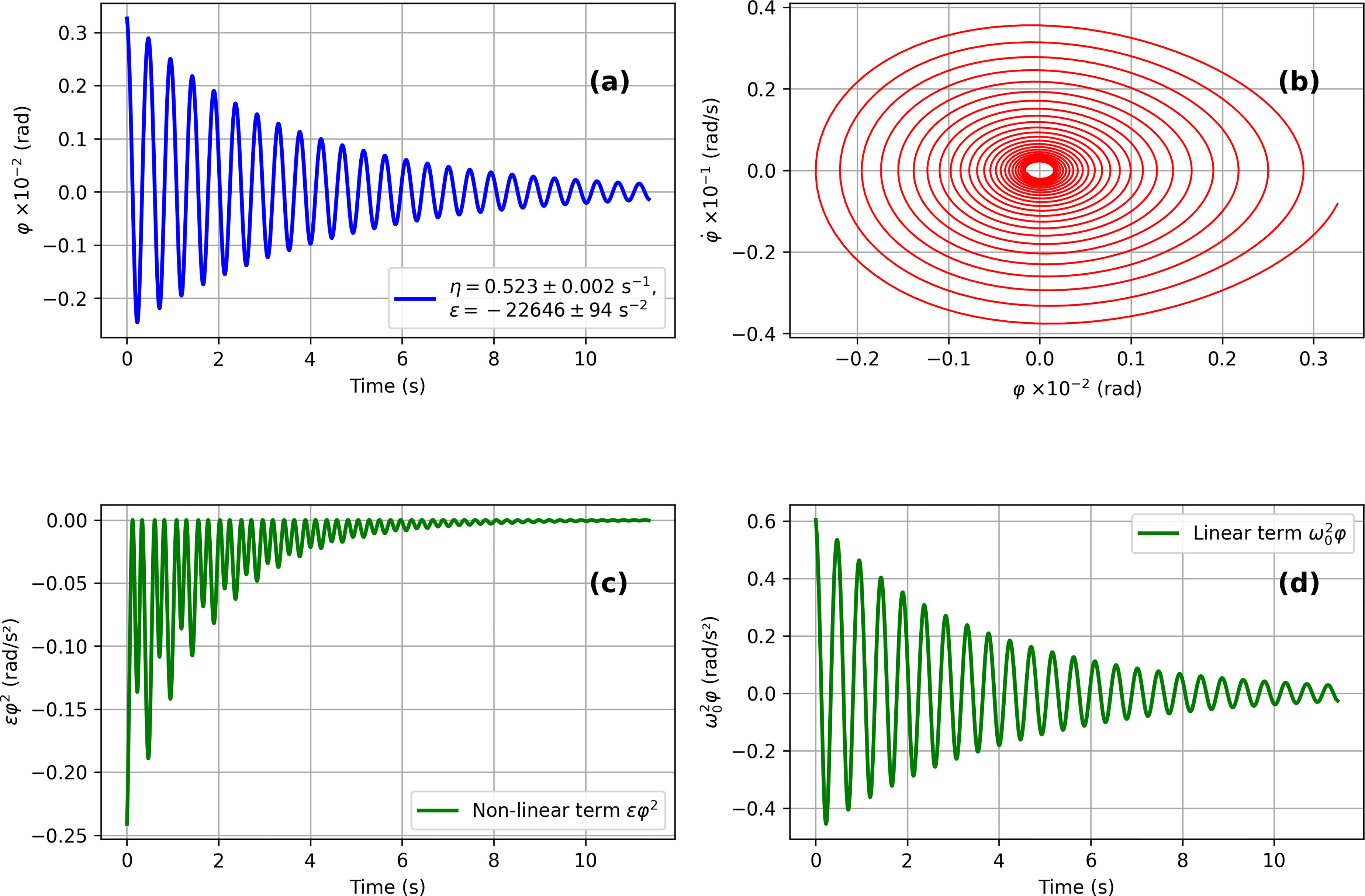
In Figure 6 we show the graphs of the integrator for Eq. (8) optimized to fit the experimental data using the program in Listing 2 of the supplemental Material. The best set of parameters that fits the experimental data is given in Table 1. In Figure 6(a) we plot the resulting angular oscillations φ(t) as a function of time t. In Figure 6(b) we plot the phase space with φ and $\stackrel{.}{\phi }$ as coordinate axis. This is typical behavior of a damped oscillator losing energy to a dissipative force until it ceases motion. In Figure 6(c) we display the contribution of the nonlinear term ϵφ², which is negative due to ϵ < 0.

Figure 6
Results of ScyPy integrator: (a) Angular position as a function of time. (b) Phase space plot $(\phi ,\stackrel{.}{\phi })$. (c) nonlinear term contribution to ODE as a function of time. (d) Linear term contribution to ODE as a function of time.

Table 1
Set of experimental parameters and the parameters optimized by the integrator in SciPy.

Parameter	Exp.	Optimized
φ0 (10−2rad)	0.196±0.002	0.3263±0.0009
η (s−1)	0.520±0.002	0.523±0.002
ω0 (rad/s)	17±2	13.603±0.002
ϵ (s−2)	−177 ± 11	−22646 ± 94

It is interesting to note that the main contribution of the nonlinear term is more expressive in the first half of the data acquisition time. In Figure 6(d) we plot the contribution to ODE of the linear term ${\omega }_0^2\phi$, which is larger than the nonlinear contribution at all times. Note that the number of oscillations of the nonlinear contribution is apparently twice the number of oscillations of the linear contribution. To investigate this, we performed a fast Fourier transform of the experimental data and observed a second small and pronounced peak at 2ω₀. Although this secondary peak is much smaller than the main contribution from ω₀, this evidence corroborates what is seen in the graph. We display the FFT plot with respect to the frequency in a log scale in the small figure inside the Figure 7. As one can see, there is a first pronounced peak at f₀ = 2.1 Hz and other exactly at 2f₀ = 4.2 Hz, corresponding to ω₀ = 2πf₀ ≈ 13.2 rad/s and 26.4 rad/s, respectively.

Figure 7
Curve fitting of Eq. (8) to experimental data with optimized parameters.

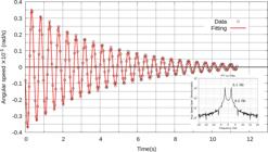
The resulting fit of Eq. (8) to experimental data with optimized parameters can be seen in Figure 7. We can say that there is a relatively good agreement between experimental data and Eq. (8). The correlation value of the fit is r² = 0.992 with the sum of the square of residuals equal to 0.002, which implies a mean square error MSE ≈1×10⁻⁶. This corroborates the hypothesis we made of integrating the Rayleigh dissipation function along the bar to obtain the dissipative force as a generalized force in the Lagrangian formalism.

5. Conclusion

We implemented the experiment of a nonlinear circular oscillator using Arduino together with the MPU6050 sensor on an Airflow 3B-Scientific circular bed kit. We discuss the physical implications from a theoretical point of view in the Lagrangian formalism, obtaining the correct equation of motion to describe the system. We assumed the hypothesis of the Rayleigh dissipation function acting on each macroscopic piece of the bar and integrated this relation to obtain the generalized dissipative force, which proved to be satisfactory to the proposed problem. This was demonstrated through the final fit of the experimental data with optimized parameters of the theoretical equation of motion, using SciPy optimization functionality for ordinary differential equations. The codes used in this work can be found in the supplemental Material. Other experimental configurations can be performed to study such a system, such as the ultrasound sensor to measure the oscillations of the weights, but this will be done in future work.

Supplementary Material

The following online material is available for this article:

I. Arduino program; II. Python code to fit experimental data.

Data Availability

The entire data set supporting the results of this study was published in the article itself.

Referências

• ^[1] E. Correa, J.S.E. Ortiz, M. Valério and J. Dutra, Revista Brasileira de Ensino de Física 33, 4307 (2011).
• ^[2] A. Beléndez, C. Pascual, D.I. Méndez, T. Beléndez and C. Neipp, Revista Brasileira de Ensino de Física 29, 645 (2007).
• ^[3] V.P. de Barros, Revista Brasileira de Ensino de Física 29, 549 (2007).
• ^[4] L.D. Landau and E. Lifchitz, Curso de física mecânica (Hemus, São Paulo, 2004).
• ^[5] S.T. Thornton and J.B. Marion, Dinâmica Clássica de Partículas e Sistemas (Cengage Learning, São Paulo, 2018).
• ^[6] H. Goldstein, C. Poole and J. Safko, Classical Mechanics (Addison-Wesley, Massachusetts, 2001).
• ^[7] 3B Scientific, Sistema rotativo de apoio pneumático, disponível em: https://www.3bscientific.com/br/sistema-rotativo-de-apoio-pneumatico-1000782-u8405680-230-3b-scientific,p137514303.html (acesso em setembro 2025).
  » https://www.3bscientific.com/br/sistema-rotativo-de-apoio-pneumatico-1000782-u8405680-230-3b-scientific,p137514303.html
• ^[8] Last Minute Engineers, MPU6050 Accelerometer and Gyroscope with Arduino Tutorial, disponível em: https://lastminuteengineers.com/mpu6050-accel-gyro-arduino-tutorial/ (acesso em setembro 2025).
  » https://lastminuteengineers.com/mpu6050-accel-gyro-arduino-tutorial/
• ^[9] P.D.M. Pereira and M.S. da Silva, Revista Brasileira de Ensino de Física 43, e20210186 (2021).
• ^[10] P.M.M. da Costa and M.B. Rocha, Ensino, Saúde e Ambiente 11, 32 (2018).

Edited by

• Editor-in-Chief:
  Marcello Ferreira https://orcid.org/0000-0003-4945-3169

Publication Dates

• Publication in this collection
  24 Oct 2025
• Date of issue
  2025

History

• Received
  14 June 2025
• Reviewed
  18 Aug 2025
• Accepted
  04 Sept 2025