GLOBAL OPTIMIZATION ALGORITHM FOR SOLVING INTEGER LINEAR FRACTIONAL MULTIPLICATIVE PROGRAMMING PROBLEMS

ABSTRACT

The Integer Linear Fractional Multiplicative Programming (ILFMP) problem, in which the objective function consists of a sum of products of linear fractional terms, is particularly challenging due to the combinatorial and non-convex nature of both the objective function and the constraint set. In this paper, we propose a method that reformulates the problem as a multiobjective integer linear fractional programming problem. We develop a Branch-and-Cut algorithm that computes the optimal solution directly, without requiring full enumeration of the efficient solutions of the associated multiobjective problem. The proposed cutting planes eliminate dominated regions of the search space, thereby accelerating the identification of the global optimal solution.

Keywords:
Multiobjective programming; Fractional programming; Integer programming; Branch-and-cut; Nonlinear programming

1 INTRODUCTION

Multiplicative programming refers to a class of optimization problems that involve products of functions in the objective function and/or constraints. These problems are part of global optimization and are known to be NP-hard, even when restricted to linear or affine functions (Matsui, 1996). Multiplicative programming has found applications in various fields, including finance and economic analysis (Henderson & Quandt, 1985; Konno & Inori, 1989), as well as geometric optimization problems (Kuno, 1993).

The simplest subclass of multiplicative programming is the linear multiplicative program, which involves only two terms in the product within the objective function. This problem was first studied by Swarup (1966), and later investigated by other researchers (Pardalos, 1990; Konno & Kuno, 1992). Despite its apparent simplicity, the objective function remains neither convex nor concave. In fact, it is quasi-concave over regions of the feasible set where both terms share the same sign, and quasi-convex otherwise (Swarup, 1966). A more general linear version of this problem, where the objective is a sum of products of affine terms, has been studied recently by Shen et al. (2020), where the authors proposed a global branch-and-bound algorithm with linear relaxations. This formulation, known as linear multiplicative programming (LMP), arises in financial optimization (Maranas et al., 1997), plant layout design (Quesada & Grossmann, 1996), data mining and pattern recognition (Bennett & Mangasarian, 1994), chip design (Dorneich & Sahinidis, 1995), network flows (Cambini & Sodini, 2014), and robust engineering applications (Mulvey et al., 1995).

In this paper, we consider a more general case: the Integer Linear Fractional Multiplicative Programming (ILFMP) problem, which can be formulated as follows:

$\left(ILFMP\right)\left\{\begin{array}{l}\max \varphi \left(x\right)=\sum _{i=1}^r\left(\frac{c^{i}x+{\alpha }^i}{d^{i}x+{\beta }^i}·\frac{c^{r+i}x+{\alpha }^{r+i}}{d^{r+i}x+{\beta }^{r+i}}\right),\\ \text{s.t.}x\in \mathcal{X}\cap {\mathrm{\mathbb{Z}}}^n,\end{array}\right.$ (1)

where r is the number of multiplicative terms in the sum (involving 2r linear fractional expressions); c ⁱ , d ⁱ are 1 × n real row vectors; and α ⁱ , β ⁱ are scalars for each i ∈ {1, 2, . . . , 2r}. The feasible set is defined as 𝒳 = {x ∈ ℝⁿ | Ax ≤ b, x ≥ 0}, where A is an m × n real matrix and b ∈ ℝ^m .

Throughout this article, we define:

$h_i\left(x\right)=\frac{c^{i}x+{\alpha }^i}{d^{i}x+{\beta }^i},i\in \{1,\dots ,2r\},$

and assume that 𝒳 is a non-empty compact polyhedral set in ℝⁿ , and that 𝒟 = 𝒳 ∩ ℤⁿ is non-empty. Additionally, we assume that h _i (x) > 0 for all x ∈ 𝒳 and for all i ∈ {1, 2, . . . , 2r}.

Problem (1) can be equivalently expressed as:

$\left\{\begin{array}{l}\max \varphi \left(x\right)=\sum _{i=1}^r{h}_i\left(x\right)h_{r+i}\left(x\right),\\ \text{s.t.}x\in \mathcal{D}.\end{array}\right.$

This problem appears naturally in many real-world applications, especially in areas like economics, finance, engineering design, and resource allocation, where performance measures often depend on ratios of linear quantities-such as cost-benefit, efficiency, or return-on-investment (see, e.g., Charnes & Cooper, 1962; Konno & Fukaishi, 2000; Kuno, 2002). To illustrate concretely, consider a portfolio selection problem with n assets and r investment sectors. For each sector i, the decision-maker evaluates two performance ratios: a return-to-risk ratio h _i (x) = (c ⁱ x + α ⁱ )/(d ⁱ x + β ⁱ ), where c ⁱ captures expected returns and d ⁱ represents risk exposure, and a liquidity-to-cost ratio h _r+i (x) = (c ^r+i x + α ^r+i )/(d ^r+i x + β ^r+i ), where c ^r+i reflects asset liquidity and d ^r+i encodes transaction costs. The product h _i (x)h _r+i (x) captures the overall attractiveness of sector i, combining risk-adjusted returns with liquidity efficiency. The total portfolio performance is then $\varphi \left(x\right)=\sum _{i=1}^r{h}_i\left(x\right)h_{r+i}\left(x\right)$, which matches the ILFMP objective (1). Here, the integer constraints reflect indivisible investment units (e.g., lots of shares), and the feasible set constraints include budget limits, diversification requirements, and risk exposure bounds (see Landsman et al., 2018, for a generalized measure using fractional expressions). In agriculture, similar models have been used to allocate water resources by coordinating different factors such as crop needs and water productivity (Zhao et al., 2017). Another example is the sum product ratio problem studied by Wang (2016), which can be applied to situations like consumer behavior, where a person selects a group of products to evaluate while considering the cost of searching, or project assignments, where success depends on all teams involved performing well. For a more comprehensive survey on the applications and developments in fractional programming, we refer the reader to Stancu-Minasian (2012) and Stancu-Minasian (2019).

This class of problems belongs to global optimization and is known to be NP-hard due to its non-convex and combinatorial nature (Benson, 1998; Pardalos & Phillips, 1991). To the best of our knowledge, no existing work addresses specifically the integer formulation involving a sum of multiple products of linear fractional terms. However, within the multiplicative programming literature, several global solution strategies have been developed for the linear multiplicative programming (LMP) problem with continuous variables. Notably, Zhao & Zhao (2018) and Shen et al. (2020) proposed branch-and-bound-based global optimization algorithms, and more recently, Cambini et al. (2023) and Huang & Gao (2023) developed efficient branch-and-bound algorithms using outer space and criterion space search strategies.

More recently, Ghasemi Saghand & Charkhgard (2022) and Ghasemi Saghand et al. (2022) studied the Integer Linear Generalized Maximum Multiplicative Program (IL-GMMP), in which the objective is a product of linear (affine) terms subject to integer constraints. Their approach reformulates the problem through the lens of multiobjective optimization and proposes exact solution methods, including a reformulation as a Mixed-Integer Second-Order Cone Program (MISOCP). However, their work is restricted to products of linear functions and does not address the fractional (ratio) structure that characterizes our ILFMP formulation. In particular, the MISOCP reformulation they employ cannot be extended to the product-of-ratios setting, since the ratio structure precludes a direct second-order cone representation.

We also note that each product term h _i (x)h _r+i (x) in the ILFMP objective can be expressed as a ratio of quadratic functions, which connects our model to the broader class of quadratic fractional programs. Optimality conditions for multiobjective quadratic fractional optimization have been studied by de Oliveira et al. (2019), who established necessary and sufficient conditions for global Pareto optimality. However, the ILFMP possesses a specific decomposable structure, where each quadratic ratio factors as a product of two linear ratios, which our method exploits through a multiobjective linear fractional reformulation. This decomposition allows us to leverage simplex-based algorithms for linear fractional programs, which are not directly available in the general quadratic fractional setting.

Within the literature on integer fractional programming, several related works employ branch-and-cut frameworks based on multiobjective reformulations. Chaiblaine & Moulaï (2024) developed an exact method for maximizing a sum of linear ratios over integer feasible sets, where the scalar problem is reformulated as a multiobjective integer linear fractional program and solved via a branch-and-cut procedure. Moreover, while the suggested approach shares the general branch-and-cut family and efficiency test mechanism with these works, it addresses a fundamentally different problem class: the ILFMP involves a sum of products of linear ratios, rather than a sum or individual ratios. In other words, the formulation addressed in this work can be considered as a generalized form of the sum of linear ratios problem. Cherfaoui & Moulaï (2021) proposed a method for generating the complete efficient set of a multiobjective integer linear plus linear fractional program. Furthermore, Chaiblaine et al. (2020) addressed the optimization of two linear fractional functions over the efficient set of a multiobjective integer linear fractional program.

In this paper, we propose a method that computes a global optimum for the ILFMP problem based on a multiobjective integer programming approach. It employs a Branch-and-Cut framework that combines the branch-and-bound search strategy with a cutting-plane technique. This enables us to avoid full enumeration of the efficient set and instead focus the search on promising regions containing global optimal solutions.

The main contributions of this paper are threefold:

1. We address, for the first time, the Integer Linear Fractional Multiplicative Programming (ILFMP) problem, a class that generalizes both the integer linear multiplicative programs studied by Ghasemi Saghand & Charkhgard (2022) and the continuous fractional multiplicative programs considered by Shen et al. (2020) and Zhao & Zhao (2018).

2. We establish a theoretical link between the ILFMP and a Multiobjective Integer Linear Fractional Program (MOILFP), proving that the global optimal solution of the ILFMP lies within the efficient set of the associated MOILFP (Proposition 1). This reformulation enables us to exploit multiobjective optimization techniques for solving the original nonlinear problem.

3. We develop a tailored Branch-and-Cut algorithm that uses cutting planes derived from the reduced gradients of the fractional objectives in the multiobjective problem. These efficient cuts eliminate dominated regions of the search space without requiring full enumeration of the efficient set, leading to significant computational savings.

The rest of this paper is organized as follows. After this introduction, we present some preliminaries. Then we introduce the proposed algorithm, followed by the main theoretical results in Section 4. Next, we provide a didactic example and computational experiments. Finally, we conclude with some final remarks.

2 PRELIMINARIES

The method presented in this paper leverages the connection between ILFMP (1) and the following Multiobjective Integer Linear Fractional Program (MOILFP):

$\left\{\begin{array}{llcl}\max & h_1\left(x\right)& =& \frac{c^{1}x+{\alpha }^1}{d^{1}x+{\beta }^1},\\ & ⋮& & \\ \max & h_r\left(x\right)& =& \frac{c^{r}x+{\alpha }^r}{d^{r}x+{\beta }^r},\\ \max & h_{r+1}\left(x\right)& =& \frac{c^{r+1}x+{\alpha }^{r+1}}{d^{r+1}x+{\beta }^{r+1}},\\ & ⋮& & \\ \max & h_{2r}\left(x\right)& =& \frac{c^{2r}x+{\alpha }^{2r}}{d^{2r}x+{\beta }^{2r}},\\ \text{s.t.}& x& \in & \mathcal{D}.\end{array}\right.$ (3)

Definition 1.A feasible solution x^∗ ∈ 𝒟 is called an efficient solution of the MOILFP problem if there does not exist any other feasible solution x ∈ 𝒟 such that

$h_i\left(x\right)\ge h_i\left(x^{*}\right)\forall i\in \{1,\dots ,2r\},$

with strict inequality for at least one k ∈ {1,..., 2r}. In such a case, the criterion vector h(x) dominates h(x ^∗), where h(x) = (h _i (x))_i=1,...,2r .

Let 𝒳_E denote the set of all efficient solutions of the multiobjective integer linear fractional problem (3).

Remark 1.Efficient solutions are also commonly referred to as Pareto-optimal or nondominated solutions in the broader optimization literature (see, e.g.,Ehrgott, 2005). In this paper, we adopt the terminology “efficient solutions,” which is standard in the multiobjective integer programming community.

Proposition 1. An optimal solution of problem (1) is an efficient solution of problem (3).

Proof. Let x ^∗ be an integer optimal solution of problem (1). Suppose, for contradiction, that x ^∗ is not an efficient solution of (3). Then there exists another feasible solution $\overline{x}\in \mathcal{D}$ such that

$h_i\left(\overline{x}\right)\ge h_i\left(x^{*}\right)\text{for all}i\in \{1,\dots ,2r\},$

with strict inequality for at least one index j ∈ {1,..., 2r}.

From the assumption that h _i (x) > 0 for all x ∈ 𝒳 and i ∈ {1,..., 2r}, we deduce that:

$h_i\left(x^{*}\right)h_{r+i}\left(x^{*}\right)\le h_i\left(\overline{x}\right)h_{r+i}\left(\overline{x}\right)\text{for all}i\in \{1,\dots ,r\}.$

Furthermore, since $h_j\left(\overline{x}\right)>h_j\left(x^{*}\right)$ for at least one j ∈ {1,..., 2r}, there must exist at least one index k ∈ {1,..., r} (where k = j if j ≤ r, or k = j − r if j > r) such that:

$h_k\left(x^{*}\right)h_{r+k}\left(x^{*}\right)<h_k\left(\overline{x}\right)h_{r+k}\left(\overline{x}\right).$

Adding these inequalities over i = 1 to r, we obtain:

$\sum _{i=1}^r{h}_i\left(x^{*}\right)h_{r+i}\left(x^{*}\right)<\sum _{i=1}^r{h}_i\left(\overline{x}\right)h_{r+i}\left(\overline{x}\right),$

which implies that

$\varphi \left(x^{*}\right)<\varphi \left(\overline{x}\right).$

This contradicts the assumption that x ^∗ is an optimal solution of (1), completing the proof. □

Corollary 1.If a feasible solution x ∈ 𝒟 is dominated for problem (3), then x is not an optimal solution of problem (1).

Proof. Suppose x ∈ 𝒟 is dominated. Then there exists another feasible solution $\overline{x}\in \mathcal{D}$ such that $h_i\left(\overline{x}\right)\ge h_i\left(x\right)$ for all i ∈ {1,..., 2r}, with strict inequality for at least one index j ∈ {1,..., 2r}. Since h _i (z) > 0 for all z ∈ 𝒳 and i ∈ {1,..., 2r}, we obtain:

$h_i\left(\overline{x}\right)h_{r+i}\left(\overline{x}\right)\ge h_i\left(x\right)h_{r+i}\left(x\right)\text{for all}i\in \{1,\dots ,r\}.$

Furthermore, because of the strict inequality at index j, there exists at least one index k ∈ {1,..., r} (with k = j if j ≤ r, or k = j − r if j > r) such that $h_k\left(\overline{x}\right)h_{r+k}\left(\overline{x}\right)>h_k\left(x\right)h_{r+k}\left(x\right)$. Summing these inequalities from i = 1 to r, we have:

$\sum _{i=1}^r{h}_i\left(\overline{x}\right)h_{r+i}\left(\overline{x}\right)>\sum _{i=1}^r{h}_i\left(x\right)h_{r+i}\left(x\right),$

which implies that $\varphi \left(\overline{x}\right)>\varphi \left(x\right)$. Therefore, x cannot be an optimal solution of problem (1). □

Definition 2.The ideal point is the vector$({\overline{h}}_1,\dots ,{\overline{h}}_{2r})$, where each component${\overline{h}}_i$represents the maximum value of h _i (x) over the feasible set 𝒟, i.e.,

${\overline{h}}_i=\underset{x\in \mathcal{D}}{\max }{h}_i\left(x\right),\text{for all}i\in \{1,\dots ,2r\}.$

Proposition 2.The optimal value ϕ* of problem (1) satisfies${\varphi }^{*}\le \overline{\varphi }$, where$\overline{\varphi }=\sum _{i=1}^r{\overline{h}}_i{\overline{h}}_{r+i}$is the sum of products of corresponding components of the ideal point.

Proof. Since $h_i\left(x\right)\le {\overline{h}}_i$ for all x ∈ 𝒳 and i ∈ {1,..., 2r}, it follows that

$\varphi \left(x\right)=\sum _{i=1}^r{h}_i\left(x\right)h_{r+i}\left(x\right)\le \sum _{i=1}^r{\overline{h}}_i{\overline{h}}_{r+i}=\overline{\varphi },\forall x\in \mathcal{X}.$

Thus, ${\varphi }^{*}\le \overline{\varphi }$. □

While the efficient set of (3) contains an optimal solution of (1), generating the full set is often computationally infeasible due to its potentially large size. To address this, the proposed method incorporates efficient cuts (Chergui & Moulaï, 2008) to prune dominated regions of the search space and uses bounding techniques to avoid exhaustive exploration of the efficient set.

Consequently, the exploration of the feasible domain is organized as a search tree. At each node, a continuous linear fractional program (LFP_l) (4) is solved over a recursively partitioned region 𝒳_l, where 𝒳₀ = 𝒳 denotes the feasible domain of problem (3) without the integrality constraints.

$\left({\text{LFP}}_l\right)\left\{\begin{array}{llcl}\max & h_1\left(x\right)& =& \frac{c^{1}x+{\alpha }^1}{d^{1}x+{\beta }^1},\\ \text{s.t.}& x& \in & {\mathcal{X}}_l.\end{array}\right.$ (4)

Without loss of generality, any objective function h _i (x), i ∈ {1,..., 2r} may be selected at this stage instead of h ₁(x).

If the solution found is integer, an efficient cut is applied; otherwise, the feasible set is partitioned into two mutually exclusive and complementary subdomains.

2.1 Characterization of Efficiency for the Multiobjective Linear Fractional Programming

When the optimal basic feasible solution x ^∗ of problem (4) is integer, we have to verify whether x ^∗ ∈ 𝒳_E by solving the following mixed integer linear program:

$\text{MM}\left(x^{*}\right)\left\{\begin{array}{llcl}\max & \Psi & =& \sum _{i=1}^{2r}{\psi }_i,\\ \text{s.t.}& [c^i-h_i(x^{*}\left)d^i\right]x-{\psi }_i& =& h_i\left(x^{*}\right){\beta }^i-{\alpha }^i,\forall i\in \{1,\dots ,2r\},\\ & x& \in & \mathcal{D},\\ & {\psi }_i& \ge & 0,\forall i\in \{1,\dots ,2r\}.\end{array}\right.$ (5)

where $h_i\left(x^{*}\right)=\frac{N_i\left(x^{*}\right)}{D_i\left(x^{*}\right)}=\frac{(c^i{x}^{*}+{\alpha }^i)}{(d^i{x}^{*}+{\beta }^i)}$, i ∈ {1,..., 2r}.

Theorem 1. A solution x ^∗ is efficient for the MOILFP problem if and only if the optimal objective value of problem (5) is zero.

Proof. Let (x, ψ) be a feasible solution of problem (5). For each i ∈ {1,..., 2r}, we have:

${\psi }_i\ge 0\iff [c^i-h_i(x^{*}\left)d^i\right]x-h_i\left(x^{*}\right){\beta }^i+{\alpha }^i\ge 0\iff h_i\left(x\right)\ge h_i\left(x^{*}\right).$

Now suppose $\Psi =\sum _{i=1}^{2r}{\psi }_i>0$. Then there exists some j ∈ {1,..., 2r} such that ψ _j > 0, implying h _j (x) > h _j (x ^∗). Thus, x dominates x ^∗, so x ^∗ is not efficient.

Conversely, suppose (x, ψ) is an optimal solution of (5) with Ψ = 0. Then ψ _i = 0 for all i, and:

$[c^i-h_i(x^{*}\left)d^i\right]x-h_i\left(x^{*}\right){\beta }^i+{\alpha }^i=0\Rightarrow h_i\left(x\right)=h_i\left(x^{*}\right),\forall i.$

Therefore, no other solution strictly improves any objective, so x ^∗ is efficient. □

Remark 2.In the above theorem, the solution x^∗is not assumed to be efficient a priori; it is any integer feasible solution encountered during the branching process. Problem (5) serves as an active test to determine whether x^∗is efficient or dominated. Specifically, the test cannot return a weakly efficient solution as a false positive for efficiency: if Ψ* = 0, then ψ _i = 0 for all i, meaning no feasible solution x ∈ 𝒟 satisfies h _i (x) ≥ h _i (x ^∗) with at least one strict inequality. This corresponds strictly to the definition of efficiency (Definition 1), not weak efficiency. Note that if Ψ* > 0, the corresponding optimal solution of problem (5) is a feasible solution that dominates x ^∗ , but it is not necessarily efficient itself due to the scaling of the variables by the denominators. To obtain an efficient solution from x ^∗ , one would need to solve the test iteratively until Ψ* = 0. However, obtaining an efficient solution when x ^∗ is dominated is not required in our algorithm; the test is strictly used as a decision tool to verify whether the candidate solution x ^∗ is efficient or not.

2.2 The Reduced Gradients of the Fractional Objectives

The method involves solving a sequence of continuous linear fractional maximization programs (4).

Let x ^∗(l) be a solution obtained after solving the problem (4) and let ℬ_(l) and 𝒩_(l) denote, respectively, the index set of basic variables and the index set of non-basic variables of the optimal solution x ^∗(l) .

We define the vectors:

$$\begin{gathered} {\nu }^{i\left(l\right)}=c^i-c_{{\mathcal{B}}_l}^i{B}_l^{-1}A, \\ {\mu }^{i\left(l\right)}=d^i-d_{{\mathcal{B}}_l}^i{B}_l^{-1}A, \end{gathered}$$

where ℬ_l denotes the index set of basic variables and B _l is the corresponding basis matrix at iteration l.

Recall that N _i (x) = c ⁱ x + αi and D _i (x) = d ⁱ x + β ⁱ denote the numerator and denominator of h _i (x), respectively. For each non-basic index j ∈ 𝒩_(l) , the reduced gradient of h _i (x) is defined as:

${\gamma }_j^{i\left(l\right)}=D_i\left(x^{*\left(l\right)}\right){\nu }_j^{i\left(l\right)}-N_i\left(x^{*\left(l\right)}\right){\mu }_j^{i\left(l\right)}.$

The following theorem (Martos, 1964) gives us the optimality condition for problem (4):

Theorem 2.A basic feasible solution x^∗(l)is optimal for problem (4) if and only if the reduced gradient of the maximized objective satisfies${\gamma }_j^{1\left(l\right)}\le 0$for all j ∈ 𝒩_(l) .

3 THE PROPOSED METHOD

Proposition 1 guarantees that the global optimal solution of (1) lies within the set of non-dominated solutions 𝒳_E of (3). Moreover, its contrapositive also holds, as formalized in Corollary 1: any dominated solution of (3) cannot be optimal for (1).

Unlike standard scalarization techniques that convert a multiobjective problem into a single-objective one, our approach proceeds in the reverse direction. This is motivated by the computational difficulty of the ILFMP: the objective function is non-convex and involves products of linear fractional terms. Direct optimization approaches (such as spatial branch-and-bound) must handle these nonconvexities via bilinear relaxations, which often lead to loose bounds and large search trees. By reformulating the problem as a MOILFP, we decompose the objective into individual linear fractional terms, allowing us to solve the continuous relaxations as linear fractional programs (LFPs) in polynomial time using simplex-based methods (Martos, 1964; Cambini & Martein, 1992). Proposition 1 and Corollary 1 guarantee that this reformulation preserves global optimality regardless of whether the objectives h ₁ , . . . , h _2r are conflicting.

Therefore, our method combines a branch-and-bound procedure with a cutting plane strategy specifically designed to eliminate dominated regions of the feasible space, thereby focusing the search on areas potentially containing non-dominated solutions.

The branching process. The search for optimal solutions follows an implicit enumeration scheme organized as a tree. At each node, the objective function h ₁ is selected for optimization using a simplex-based procedure (Martos, 1964; Cambini & Martein, 1992).

At node l, we solve the continuous relaxation (LFP_l ) over domain 𝒳_l , starting from 𝒳₀ = 𝒳.

Since h ₁ is linear fractional and 𝒳 is bounded, (LFP_l ) either has no feasible solution or attains an optimal value.

• - If (LFP_l ) is infeasible, node l has no children and is fathomed.

• - If an optimal solution x ^∗(l) is found:

• - If x ^∗(l) is not integer, standard branch-and-bound techniques are applied: select a fractional variable $x_k^{*\left(l\right)}$, and create two subproblems with added constraints $x_k\le \lfloor x_k^{*\left(l\right)}\rfloor$ and $x_k\ge \lceil x_k^{*\left(l\right)}\rceil$.

• - If x ^∗(l) is integer, it is tested for efficiency via problem (5), and the current best objective value ϕ _opt is updated accordingly.

Updating the optimal value. The algorithm maintains a lower bound ϕ _opt (initialized to −∞) and an upper bound ϕ _upper, computed at each node using the ideal point.

At node l, if (LFP_l ) yields a solution x ^∗(l) , compute ${\varphi }_{\text{upper}}=\sum _{i=1}^r{\overline{h}}_i{\overline{h}}_{r+i}$, where $\{{\overline{h}}_1,\dots ,{\overline{h}}_{2r}\}$ is the ideal point at this node. This upper bound is justified by Proposition 2. Although the bound could be stated directly, calculating the ideal point at each node of the Branch-and-Cut algorithm provides a natural, readily available upper bound to prune unpromising subproblems without requiring additional optimization steps.

If x ^∗(l) is integer, test its efficiency using (5). If it is efficient and ϕ (x ^∗(l) ) > ϕ _opt, update ϕ _opt and record x ^∗(l) as the current best solution.

The cutting plane method. If the solution x ^∗(l) is integer, we construct an efficient cut to eliminate all solutions whose criterion vector is dominated by h(x ^∗(l) ). This cut takes the form:

$\sum _{j\in {\mathcal{H}}_l}{x}_j\ge 1,$

where

${\mathcal{H}}_l=\left\{j\in {\mathcal{N}}_l\mid \exists i\in \{2,\dots ,2r\},{\gamma }_j^{i\left(l\right)}>0\right\}\cup \left\{j\in {\mathcal{N}}_l\mid {\gamma }_j^{i\left(l\right)}=0,\forall i\right\}.$

If ${\mathcal{H}}_l=\varnothing$, the current domain contains no further improving solutions, and the node is fathomed. Otherwise, the constraint is added to the child node l ₀.

Rules for fathoming nodes. A node is fathomed if:

• - (LFP_l ) is infeasible;

• - ϕ _upper ≤ ϕ _opt;

• - x ^∗(l) is integer and ${\mathcal{H}}_l=\varnothing$, indicating no further efficient solutions remain in the current domain.

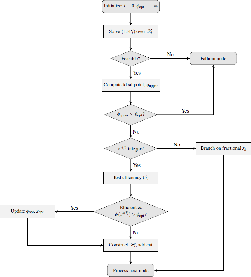
Algorithm 1 summarizes the complete steps of the proposed method. The nodes within its tree structure can be explored using standard traversal strategies, such as depth-first search or back-tracking. Additionally, Figure 1 provides a flowchart summarizing the main steps and decision points of the Branch-and-Cut procedure.

Algorithm 1:
ILFMP Optimization Algorithm

Result: Global optimal solution x opt of (1)

Initialization: l = 0, 𝒳0 = 𝒳, ϕ opt = −∞, x opt unknown;

while there exists a non-fathomed node n l do

| Solve (LFPl ):

| $\left({\text{LFP}}_l\right)\left\{\begin{array}{ll}\max & h_1\left(x\right)\\ \text{s.t.}& x\in {\mathcal{X}}_l\end{array}\right.;$

| if (LFP l ) has an optimal solution x ∗(l) then

| | Compute local ideal point $({\overline{h}}_1,\dots ,{\overline{h}}_{2r})$ and set ${\varphi }_{\text{upper}}=\sum _{i=1}^r{\overline{h}}_i{\overline{h}}_{r+i}$;

| | if ϕ upper ≤ ϕ opt then

| | | Fathom node n l ;

| | end

| | if x ∗(l) is integer then

| | | Test efficiency of x ∗(l) by solving problem (5);

| | | if x ∗(l) is efficient then

| | | | if ϕ(x ∗(l) ) > ϕ opt then

| | | | | Update ϕ opt = ϕ (x ∗(l) );

| | | | | Set x opt = x*(l) ;

| | | | end

| | | end

| | | Construct ℋl ;

| | | if${\mathcal{H}}_l=\varnothing$then

| | | | Fathom node n l

| | | else

| | | | Add cut $\sum _{j\in {\mathcal{H}}_l}{x}_j\ge 1$ to child node n l’ ;

| | | end

| | else

| | | Choose index k such that $x_k^{*\left(l\right)}$ is fractional;

| | | Create nodes $n_{l_1},n_{l_2}$ with constraints $x_k\le \lfloor x_k^{*\left(l\right)}\rfloor$ and $x_k\ge \lceil x_k^{*\left(l\right)}\rceil$;

| | end

| else

| | Fathom node n l ;

| end

end

Figure 1
Flowchart of the proposed Branch-and-Cut algorithm for solving the ILFMP problem.

4 THEORETICAL RESULTS

The following theoretical results demonstrate that the proposed algorithm identifies all global optimal solutions (if any exist) to problem (1) in a finite number of iterations.

Theorem 3.Let x^∗(l)be an integer solution such that${\mathcal{H}}_l\ne \varnothing$. If there exists an integer optimal solution x ∈ 𝒳_l \{x ^∗(l) }, then$x\in {\mathcal{X}}_{l_0}$, where:

${\mathcal{X}}_{l_0}=\left\{x\in {\mathcal{X}}_l|\sum _{j\in {\mathcal{H}}_l}{x}_j\ge 1\right\}.$

Proof. Assume $\overline{x}\in {\mathcal{X}}_l$ is such that $\overline{x}\ne x^{*\left(l\right)}$ and ${\overline{x}}_j=0$ for all j ∈ ℋ_l .

According to the simplex tableau at x ^∗(l) , the update in each objective h _i (x) is determined by the nonbasic indices j ∈ 𝒩_(l) . Hence, for every i ∈ {1,..., 2r}:

$$\begin{gathered} N_i\left(\overline{x}\right)=N_i\left(x^{*\left(l\right)}\right)+{\theta }_j{\nu }_j^{i\left(l\right)}, \\ {D}_i\left(\overline{x}\right)=D_i\left(x^{*\left(l\right)}\right)+{\theta }_j{\mu }_j^{i\left(l\right)}, \end{gathered}$$

where

${\theta }_j=\min \left\{\frac{x_{B_k}^{*\left(l\right)}}{a_{kj}}|a_{kj}>0,k\in I_l\right\},j\in {\mathcal{N}}_{\left(l\right)}.$

Then:

$h_i\left(\overline{x}\right)=\frac{N_i\left(x^{*\left(l\right)}\right)+{\theta }_j{\nu }_j^{i\left(l\right)}}{D_i\left(x^{*\left(l\right)}\right)+{\theta }_j{\mu }_j^{i\left(l\right)}}.$

By subtracting:

$$\begin{gathered} h_i\left(\overline{x}\right)-h_i\left(x^{*\left(l\right)}\right)={\theta }_j·\frac{D_i\left(x^{*\left(l\right)}\right){\nu }_j^{i\left(l\right)}-N_i\left(x^{*\left(l\right)}\right){\mu }_j^{i\left(l\right)}}{D_i\left(x^{*\left(l\right)}\right)D_i\left(\overline{x}\right)} \\ =\frac{{\theta }_j·{\gamma }_j^i}{D_i\left(x^{*\left(l\right)}\right)D_i\left(\overline{x}\right)}. \end{gathered}$$

Since $D_i\left(x^{*\left(l\right)}\right),D_i\left(\overline{x}\right)>0$ and ${\gamma }_j^i\le 0$ for all j ∈ 𝒩_(l) \ℋ_l (with strict inequality for at least one i), it follows:

$h_i\left(\overline{x}\right)\le h_i\left(x^{*\left(l\right)}\right),\forall i,$

with strict inequality for at least one index. Thus, $\overline{x}$ is dominated and not efficient. □

Corollary 2. The constraint $\sum _{j\in {\mathcal{H}}_l}{x}_j\ge 1$ defines an efficient cut.

Proof. By Theorem 3, all integer efficient solutions in 𝒳_l satisfy this constraint, while x ^∗(l) does not. Therefore, the constraint removes only dominated solutions and is an efficient cut. □

Proposition 3.If${\mathcal{H}}_l=\varnothing$at the current integer solution x^∗(l), then 𝒳_l \{x ^∗(l) } contains no global optimal solution.

Proof. If ${\mathcal{H}}_l=\varnothing$, then all reduced gradients ${\gamma }_j^i\le 0$ for all j ∈ 𝒩_(l) and i ∈ {1,..., 2r}. This implies that x ^∗(l) is optimal for all objectives within 𝒳_l . Hence, no other solution in 𝒳_l can dominate it, and 𝒳_l \{x ^∗(l) } contains no efficient (and thus no globally optimal) solutions. □

Theorem 4. The algorithm terminates in a finite number of iterations and returns a global optimal solution to problem (1), if one exists.

Proof. Each time an integer solution x ^∗(l) is encountered, an efficient cut is applied (when ${\mathcal{H}}_l\ne \varnothing$) that excludes x ^∗(l) and other dominated solutions, without eliminating any globally optimal solution (by Theorem 3 and Corollary 2).

Moreover, the integer feasible set 𝒟 is finite due to boundedness, and so is the set of efficient solutions 𝒳_E . As the algorithm exhaustively explores all of 𝒳_E through branching or cutting, it must terminate in finite time. □

5 DIDACTIC EXAMPLE

To better understand the proposed approach, we present a didactic example illustrating the algorithm’s operation. The selected instance is simple enough to allow a step-by-step walkthrough while still reflecting the core features and challenges of the ILFMP model.

Consider the following problem:

$\text{(ILFMP)}\left\{\begin{array}{ll}\max & \varphi \left(x\right),\\ \text{subject to:}& \\ & 8x_1+3x_2+4x_3\le 12,\\ & 2x_1+5x_2+5x_3\le 25,\\ & 4x_1+x_2+x_3\le 27,\\ & 6x_1+9x_2+7x_3\le 26,\\ & x_1,x_2,x_3\in {\mathrm{\mathbb{Z}}}_{+}.\end{array}\right.$ (6)

where the nonlinear objective function ϕ(x) is given by:

$$\begin{gathered} \varphi \left(x\right)=\frac{(14x_1+8x_2+15x_3+11)(5x_2+14x_3+11)}{(5x_1+10x_2+16x_3+17)(9x_1+20x_2+8x_3+17)} \\ +\frac{(11x_1+5x_2+7x_3+14)(16x_1+6x_2+12x_3+17)}{(13x_1+7x_2+4x_3+4)(15x_1+20x_2+2x_3+9)} \\ +\frac{(3x_1+x_2+10x_3+13)(19x_1+10x_3+20)}{(11x_1+6x_2+15x_3+4)(x_1+9x_2+4x_3+15)}· \end{gathered}$$

The corresponding multiobjective linear fractional programming problem (MOILFP), associated with problem (6), consists in maximizing the six fractional terms composing ϕ(x):

$\left(MOILFP\right)\left\{\begin{array}{l}\text{max}{h}_1\left(x\right)=\frac{14x_1+8x_2+15x_3+11}{5x_1+10x_2+16x_3+17},\\ \text{max}{h}_2\left(x\right)=\frac{5x_2+14x_3+11}{9x_1+20x_2+8x_3+17},\\ \text{max}{h}_3\left(x\right)=\frac{11x_1+5x_2+7x_3+14}{13x_1+7x_2+4x_3+4},\\ \text{max}{h}_4\left(x\right)=\frac{16x_1+6x_2+12x_3+17}{15x_1+20x_2+2x_3+9},\\ \text{max}{h}_5\left(x\right)=\frac{3x_1+x_2+10x_3+13}{11x_1+6x_2+15x_3+4},\\ \text{max}{h}_6\left(x\right)=\frac{19x_1+10x_3+20}{x_1+9x_2+4x_3+15},\\ \text{subject to: (same constraints as in}\left(6\right))\end{array}\right.$ (7)

At node l = 1, the relaxed single-objective problem (LFP ₍₁₎) is solved:

$\left(LF{P}_{\left(1\right)}\right)\left\{\begin{array}{l}\text{max}{h}_1\left(x\right)=\frac{14x_1+8x_2+15x_3+11}{5x_1+10x_2+16x_3+17},\\ \text{subject to: (same constraints as in}\left(6\right))\text{but with}{x}_1,x_2,x_3\ge 0.\end{array}\right.$ (8)

Table 1 presents the step-by-step execution of the algorithm.

Table 1
Execution steps of the algorithm applied to the didactic example. ✓denotes an efficient solution; ✗ denotes a dominated solution.

It. l	x* (l)	ϕ* (l)	Nodes Created	Efficient?	ϕ upper	ϕ opt	ℋl
1	(3/2, 0, 0)	-	(2), (3)	-	23.61	-	-
2	(1, 0, 0)	5.10	(4)	✓	21.80	5.10	(3, 8)
3	Infeasible	-	-	-	-	5.10	-
4	(1, 0, 1)	5.53	(5)	✓	21.69	5.53	(8, 9)
5	(3/4, 0, 3/2)	-	(6), (7)	-	21.00	5.53	-
6	(0, 0, 0)	11.36	(8)	✓	19.50	11.36	(2, 10, 11)
7	Infeasible	-	-	-	-	11.36	-
8	(0, 1, 0)	2.84	(9)	✓	12.98	11.36	(10, 11, 12)
9	(0, 2, 0)	-	(10)	✗ (dom. by (0, 0, 2))	12.63	11.36	(10, 11, 13)
10	(0, 2.85, 0.05)	-	(11), (12)	-	12.63	11.36	-
11	(0, 2, 1/3)	-	(13), (14)	-	12.63	11.36	-
12	Infeasible	-	-	-	-	11.36	-
13	Infeasible	-	-	-	-	11.36	-
14	(0, 0, 1)	9.62	(15)	✓	12.63	11.36	(11, 14, 16)
15	(0, 1, 1)	-	(16)	✗ (dom. by (0, 0, 2))	12.12	11.36	(11, 16, 17)
16	(0, 2, 1)	-	(17)	✗ (dom. by (0, 0, 3))	11.87	11.36	(11, 16, 18)
17	(0, 1.98, 1.17)	-	(18), (19)	-	11.73	11.36	-
18	(0, 1, 1.33)	-	(20), (21)	-	-	11.36	-
19	Infeasible	-	-	-	-	11.36	-
20	(0, 1, 2)	-	-	- (fathomed)	11.16	11.36	-
21	Infeasible	-	-	-	-	11.36	-

The algorithm terminates with an optimal solution x _opt = (0, 0, 0) and optimal value ϕ _opt = 11.36.

6 NUMERICAL EXPERIMENTS

In this section, we present numerical experiments conducted to evaluate the performance of the proposed Branch-and-Cut algorithm. All computations were carried out using Python 3.11 on an Intel i7 10th generation processor with 16 GB of RAM. The algorithm was implemented using NumPy and SciPy for numerical computations, and CPLEX for the efficiency test sub-problem (5). For each combination of parameters (r, m, n), five random test instances were generated, and the results are reported as average values. The source code, instance generator, and all benchmark instances are publicly available at https://github.com/yacinech-sys/ILFMP.

6.1 SCIP Reformulation

To provide a robust benchmark, we compare our specialized Branch-and-Cut algorithm against SCIP 8.0.0 (Bestuzheva et al., 2023), a state-of-the-art open-source solver for Mixed-Integer Nonlinear Programming (MINLP), accessed via the PySCIPOpt interface. Since SCIP is a general-purpose solver, the ILFMP must first be reformulated into a form that SCIP can handle.

Specifically, we introduce 2r auxiliary continuous variables v _k (k ∈ {1,..., 2r}), one for each linear fractional term, along with bilinear constraints that enforce the relationship between each auxiliary variable and its corresponding fractional expression:

$v_k·\left(d^{k}x+{\beta }^k\right)=c^{k}x+{\alpha }^k,\forall k\in \{1,\dots ,2r\}$ (9)

The ILFMP objective function is then expressed as:

$\max \varphi =\sum _{i=1}^r{v}_i·v_{r+i}.$ (10)

This reformulation yields a Mixed-Integer Quadratically Constrained Program (MIQCP) with 2r bilinear constraints and r bilinear terms in the objective. SCIP handles these nonconvexities through its spatial branch-and-bound engine. A time limit of 1200 seconds is imposed on all experiments.

6.2 Instance Generation

We evaluate the solvers on several classes of instances, each designed to test different aspects of the problem structure.

6.2.1 General Random Instances

Random instances are generated as follows. The constraint matrix A ∈ ℝ^m×n has entries drawn uniformly from [1, 30], and the right-hand side vector b from [60, 100]. The numerator coefficients $c_j^i$ are drawn from [0,C _max], the denominator coefficients $d_j^i$ from [0, D _max], and the intercepts α ⁱ from [0, 10]. To ensure positive denominators, the constants β ⁱ are drawn from [β _min , β _max] with β _min > 0.

We study several parameter regimes that produce qualitatively different problem structures:

1. Set A:α, c, d ∈ [0, 100], β ∈ [1, 100]. While generated similarly to Set C, these instances are limited to smaller dimensions.

2. Set B:C_max = 2000, D _max = 1500, β ∈ [0.001, 0.05]. Moderate numerator coefficients with very small denominator constants produce high-valued ratios.

3. Set C:C_max = 2000, D _max = 1500, β ∈ [1.0, 10.0]. Larger denominator constants yield more moderate ratio values, reducing the dynamic range of the objective.

4. Set D:C_max = 20000, D _max = 1500, β ∈ [0.001, 1.0]. Large coefficients combined with small denominator constants, creating numerically challenging instances.

5. Set E: These instances are designed with highly conflicting objectives. For each product term, the coefficients of its two constituent ratios are inversely correlated: for any variable, if the first ratio receives a large numerator coefficient ([50, 1000]) and a small denominator coefficient ([0, 2]), the multiplied second ratio receives the exact opposite (small numerator and large denominator). The intercepts are drawn as α ∈ [1.0, 5.0] and β ∈ [0.05, 1.0]. This structure pulls the optimization in competing directions, creating a dense efficient set.

6. Set F: These instances feature a dense, tightly constrained knapsack structure. The constraint matrix A ∈ ℝ^m×n has entries drawn uniformly from [50, 200], and the right-hand side is set to $b_i=0.15\sum _{j=1}^n{A}_{ij}$, ensuring that only approximately 15% of the variables can take non-zero values simultaneously. The numerator coefficients $c_j^i$ are drawn from [0, 100], the denominator coefficients $d_j^i$ from [1, 20], and the intercepts α ⁱ ∈ [0, 10], β ⁱ ∈ [0.01, 1]. The combination of dense, high-valued constraint coefficients with tight capacities creates a heavily constrained feasible region that differs structurally from the general random instances.

7. Set G: This set of instances is inspired by portfolio selection (Landsman et al., 2018), where the objective function naturally takes the form of a sum of products of ratios. Given n assets, each product term h _i (x) · h _r+i (x) represents the product of a return-to-risk ratio and a liquidity-to-cost ratio for a particular investment sector or horizon. Specifically:

• Numerator coefficients $c_j^i$ (returns, liquidity) are drawn from [1, 20].

• Denominator coefficients $d_j^i$ (risk, cost) are drawn from [1, 15].

• Intercepts α ⁱ ∈ [0, 10], β ⁱ ∈ [1, 10].

The constraint set includes: (i) a budget constraint limiting total investment to 60% of the total asset value; (ii) sector diversification constraints limiting allocation per sector; (iii) a risk exposure limit; and (iv) individual variable upper bounds x _j ≤ 3. The number of constraints m is determined by the instance structure and varies with n. These instances are particularly challenging for SCIP because a high number of product terms r introduces many bilinear constraints and variables into the MIQCP reformulation.

6.3 Results

The following notation is used throughout:

• r: number of product terms; m: constraints; n: variables.

• Ours (s): average CPU time of our Branch-and-Cut algorithm.

• Our Nodes: average number of nodes explored in our search tree.

• SCIP (s): average CPU time of SCIP.

• SCIP Nodes: average number of nodes in SCIP’s spatial branch-and-bound tree.

• T/O: time-out (exceeding the 1200-second limit).

6.3.1 Instances of Set A

We first evaluate the solvers on instances from Set A, where a brute-force enumeration of the entire efficient set is still tractable. Table 2 compares our method against both the brute-force approach and SCIP. The column |𝒳_E | denotes the total number of efficient solutions (obtained by brute force), $\left|{\overline{\mathcal{X}}}_E\right|$ the number explored by our algorithm, and $\sigma =\left|{\overline{\mathcal{X}}}_E\right|/\left|{\mathcal{X}}_E\right|$ the fraction of the efficient set traversed. Our algorithm consistently outperforms the brute-force method by orders of magnitude, confirming that the cutting-plane strategy effectively prunes the search space. SCIP, benefiting from its highly optimized C++ implementation, achieves fast times on these instances. However, our method remains competitive.

Table 2
Computational performance of the algorithms on small-scale Set A instances (5 instances per configuration).

r	m	n	Ours (s)	Nodes	$\left|{\overline{\mathcal{X}}}_E\right|$	BF (s)	|XE |	σ	SCIP (s)	SCIP Nodes
2	5	5	0.13	18	6	1.52	17	0.33	0.26	12
2	10	5	0.16	25	7	0.89	16	0.42	0.31	10
3	10	5	0.32	38	12	1.27	49	0.24	0.46	17
4	10	5	0.19	21	6	0.84	30	0.21	0.60	22
4	20	10	1.15	76	19	12.80	123	0.16	1.43	22
4	30	15	6.23	283	52	168.62	233	0.22	2.58	20
5	5	5	0.35	37	12	1.52	64	0.19	0.56	27
5	10	5	0.32	31	10	1.28	45	0.22	0.63	18
5	20	10	3.18	170	44	9.71	139	0.32	2.06	15
5	30	15	4.88	227	43	136.15	237	0.18	5.15	21

6.3.2 Instances with Small Denominator Constants (Set B)

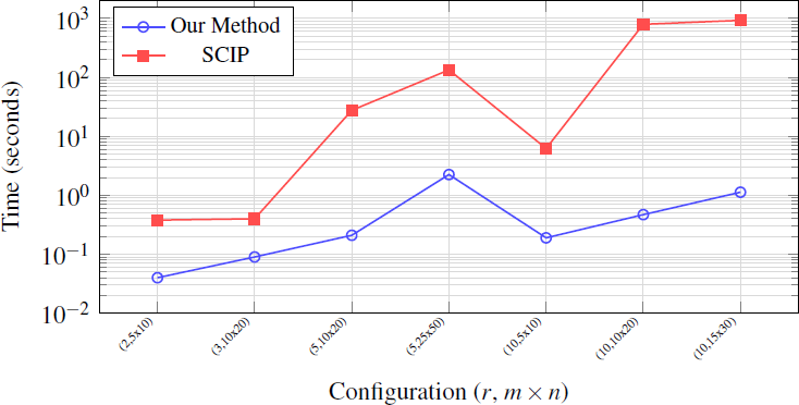
Table 3 presents results for Set B instances (C _max = 2000, β ∈ [0.001, 0.05]). The small denominator constants produce high-valued ratios, which significantly increases the difficulty for SCIP’s spatial branching. Our method dominates SCIP across all configurations, often by two to three orders of magnitude. For r = 10, m = 15, n = 30, our algorithm solves in 1.13 seconds on average, while SCIP requires over 929 seconds. The comparative execution times are visually summarized in Figure 2, illustrating the significant speedup achieved by our method.

Table 3
Set B: C ∈ [0, 2000], β ∈ [0.001, 0.05]. Average over 5 instances.

r	m	n	Ours (s)	Nodes	$\left|{\overline{\mathcal{X}}}_E\right|$	SCIP (s)	SCIP Nodes
2	5	10	0.04	7	2	0.38	16
2	10	20	0.20	27	6	0.85	345
2	15	30	0.09	16	2	1.33	96
2	20	40	0.21	30	5	0.89	128
2	25	50	0.31	34	6	1.07	170
3	5	10	0.10	11	3	0.97	966
3	10	20	0.09	10	4	0.40	55
3	15	30	0.16	17	4	1.97	284
3	20	40	0.40	36	6	1.57	118
3	25	50	0.28	24	4	1.64	123
5	5	10	0.10	10	3	0.50	82
5	10	20	0.21	18	6	27.68	1272
5	15	30	0.90	24	5	407.63	19566
5	20	40	1.26	25	6	235.55	11906
5	25	50	2.25	39	6	134.21	806
10	5	10	0.19	10	5	6.24	384
10	10	20	0.47	14	3	797.72	30777
10	15	30	1.13	16	5	929.98	65158

Figure 2
Comparison of solving times (log scale) between our method and SCIP on Set B instances (β ∈ [0.001, 0.05]). Our method dominates across all configurations, with speedups exceeding 700× for r = 10.

6.3.3 Instances with Large Denominator Constants (Set C)

Table 4 presents results for Set C (C _max = 2000, β ∈ [1.0, 10.0]). Larger denominator constants reduce the dynamic range of the fractional terms, making the SCIP reformulation more tractable. In this regime, SCIP becomes more competitive, and for some configurations with r = 2, SCIP is faster. However, as r increases beyond 5, our method’s structural advantage re-emerges. For r = 20 and larger problem sizes, both solvers require substantial time, but our method generally maintains lower or comparable runtimes.

Table 4
Set C: C ∈ [0, 2000], β ∈ [1.0, 10.0]. Average over 5 instances.

r	m	n	Ours (s)	Nodes	$\left|{\overline{\mathcal{X}}}_E\right|$	SCIP (s)	SCIP Nodes
2	5	10	2.53	94	28	1.12	296
2	10	20	1.60	65	14	2.37	374
2	15	30	2.97	108	20	4.00	1022
2	20	40	1.27	53	7	3.65	433
2	25	50	7.47	207	22	5.95	1334
3	5	10	0.26	17	5	1.12	42
3	10	20	3.11	101	21	2.50	398
3	15	30	1.54	61	14	3.07	345
3	20	40	4.12	133	20	4.34	631
3	25	50	15.52	357	42	11.99	2511
5	5	10	1.45	55	19	1.65	98
5	10	20	1.64	66	13	3.59	335
5	15	30	3.47	115	23	6.72	1026
5	20	40	7.03	168	26	10.74	1048
5	25	50	14.81	303	43	18.45	2757
10	5	10	0.93	22	8	2.66	76
10	10	20	3.27	68	16	5.46	310
10	15	30	4.49	75	17	8.12	614
10	20	40	10.60	133	23	16.80	713
10	25	50	24.27	195	37	32.74	2591
20	5	10	4.13	53	21	6.34	214
20	10	20	10.72	78	20	19.82	404
20	15	30	13.26	121	27	18.57	786
20	20	40	117.63	382	68	81.58	1908
20	25	50	86.13	181	34	137.70	2161

6.3.4 Instances of Set D

Table 5 reports results for the most challenging parameter regime: C _max = 20000, D _max = 1500, β ∈ [0.001, 1.0]. The combination of large numerator coefficients and near-zero denominator constants creates extremely high-valued fractional terms, making SCIP’s bilinear relaxations very loose. Already for r = 2, SCIP struggles significantly: at (m, n) = (10, 20), SCIP requires over 240 seconds and nearly 400,000 nodes, while our method solves in under 1.4 seconds. At (m, n) = (20, 40), SCIP times out at 1200 seconds while our method finishes in under 5 seconds.

Table 5
Set D: C ∈ [0, 20000], D ∈ [0, 1500], β ∈ [0.001, 1.0]. Average over 5 instances.

r	m	n	Ours (s)	Nodes	$\left|{\overline{\mathcal{X}}}_E\right|$	SCIP (s)	SCIP Nodes
2	5	10	2.91	91	27	7.64	13834
2	10	20	1.38	60	12	240.42	398817
2	15	30	22.63	106	19	481.71	1276305
2	20	40	4.94	103	11	T/O	-
3	5	10	0.50	16	5	544.96	459589
3	10	20	21.16	101	22	482.28	396578
3	15	30	1.15	56	12	262.43	583842
5	5	10	1.11	56	19	866.08	643617
5	10	20	4.03	53	10	T/O	-
5	15	30	7.60	122	25	1093.06	119402

6.3.5 Portfolio Selection Instances (Set G)

Table 6 reports results on portfolio selection instances. These instances feature high values of r (up to 25 product terms) with structured constraints including budget, diversification, and risk limits. The number of constraints m is determined by the portfolio structure and varies with n.

Table 6
Portfolio selection instances. Average over 3 instances per configuration.

r	m	n	Ours (s)	Nodes	$\left|{\overline{\mathcal{X}}}_E\right|$	SCIP (s)	SCIP Nodes
5	10	5	1.35	49	17	1.22	34
5	20	15	59.80	2487	635	95.06	60188
10	10	5	1.84	47	18	1.88	37
10	15	10	57.87	1079	335	26.73	2228
10	20	15	42.51	451	143	337.85	26528
15	10	5	1.15	48	16	1.71	49
15	15	10	40.98	1353	448	20.07	3070
15	20	15	531.06	13053	3926	828.31	104441
20	10	5	1.44	48	14	2.17	41
20	15	10	128.30	1761	539	27.59	2893
20	20	15	274.88	5441	1724	1081.88	62854

For small portfolios (n = 5), both solvers perform comparably. However, as the portfolio size and the number of product terms increase, SCIP’s performance degrades rapidly due to the proliferation of bilinear constraints in the MIQCP reformulation. At (r, n) = (10, 15), our method solves in 42.51 seconds while SCIP requires 337.85 seconds. At (r, n) = (15, 15), our method averages 531 seconds compared to SCIP’s 828 seconds. For the largest configuration (r, n) = (20, 15), our method completes in 275 seconds while SCIP requires over 1081 seconds, approaching the time limit. Figure 3 illustrates how the solving time scales with the number of product terms r for portfolio selection instances, highlighting SCIP’s exponential growth.

Figure 3
Portfolio selection instances with n = 15 assets: solving time (log scale) as r increases. SCIP’s runtime grows rapidly due to the proliferation of bilinear constraints, while our method scales more favorably.

We note that for moderate r with larger n (e.g., r = 10, n = 10), SCIP can outperform our method. This occurs because SCIP’s advanced presolving and primal heuristics are effective when the number of bilinear constraints is manageable, while our Python-based implementation incurs higher per-node overhead for larger constraint matrices.

6.3.6 Highly conflicting objective components (Set E)

Table 7 presents results for instances designed with highly conflicting objective components. In this parameter regime, the coefficients of the two ratios in each product term are inversely correlated: when a variable yields a large numerator and a small denominator for the first ratio, it simultaneously yields a small numerator and a large denominator for the second ratio. Combined with small denominator constants β ∈ [0.05, 1.0], this specific structure creates a highly dense efficient set with strongly competing objectives. As observed in Table 7, the performance of our algorithm deteriorates significantly compared to SCIP. The reason for this behavior is intrinsically linked to our solution mechanism: our Branch-and-Cut method relies on exploring and pruning the efficient set. When the objectives are highly conflicting, the number of efficient solutions $\left|{\overline{\mathcal{X}}}_E\right|$ grows rapidly, requiring the algorithm to generate an excessive number of cuts and explore a massive search space. By contrast, SCIP is unaffected by the multiobjective structure and solves these instances rapidly.

Table 7
Conflicting objectives instances. Average over 5 instances per configuration.

r	m	n	Ours (s)	Nodes	$\left|{\overline{\mathcal{X}}}_E\right|$	SCIP (s)	SCIP Nodes
2	5	5	2.26	82	24	0.25	20
2	5	10	33.10	868	137	0.60	126
2	5	15	72.05	1120	179	1.37	262
2	10	20	71.88	1950	211	1.47	429
3	5	5	1.92	75	26	0.35	11
3	5	10	27.68	731	170	0.74	131
3	5	15	98.87	2419	618	2.22	701
3	10	20	77.04	2298	397	2.53	550
5	5	5	2.05	85	31	0.76	23
5	5	10	14.84	501	147	2.17	208
5	5	15	98.59	2845	770	3.57	874
5	10	20	115.16	2340	501	3.95	931

6.3.7 Dense Knapsack Instances (Set F)

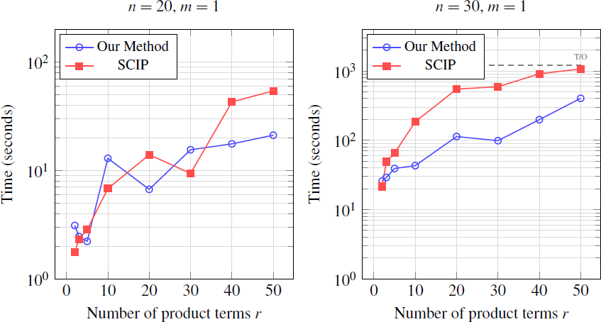
Table 8 details the performance of the algorithms on dense knapsack-style instances with a single tight knapsack constraint (m = 1). In these instances, the constraint matrix has large coefficients drawn from [50, 200] and the right-hand side is set to only 15% of the row sum, creating a heavily constrained feasible region. We vary the number of product terms from r = 2 to r = 50 to evaluate scalability. As r increases, SCIP’s performance degrades rapidly due to the proliferation of bilinear constraints in the MIQCP reformulation, while our method scales more gracefully. For n = 30 and r ≥ 20, our method achieves speedups of up to 5× over SCIP, which approaches the 1200-second time limit for r = 40 and r = 50. The performance scaling on dense knapsack instances is plotted in Figure 4, confirming that our method scales more favorably for large values of r.

Table 8
Dense knapsack instances (Set F, m = 1). Average over 5 instances per configuration.

r	n	Ours (s)	Nodes	$\left|{\overline{\mathcal{X}}}_E\right|$	SCIP (s)	SCIP Nodes
2	20	3.11	149	29	1.76	489
2	30	25.81	641	94	21.51	15952
3	20	2.46	98	23	2.33	555
3	30	29.06	856	155	49.14	28301
5	20	2.22	85	20	2.85	354
5	30	39.22	933	217	65.29	23564
10	20	12.93	274	57	6.80	644
10	30	43.10	667	167	185.0	24821
20	20	6.69	78	23	13.95	470
20	30	113.3	1164	276	548.8	39268
30	20	15.51	152	38	9.40	653
30	30	98.85	492	137	592.2	22020
40	20	17.57	65	22	42.82	541
40	30	198.5	577	174	910.4	19143
50	20	21.12	64	25	54.07	594
50	30	403.3	630	181	T/O	-

Figure 4
Dense knapsack instances (Set F): solving time (log scale) as the number of product terms r increases, for n = 20 (left) and n = 30 (right). Our method scales more favorably than SCIP, which approaches the time limit for large r with n = 30.

6.4 Discussion

The computational experiments reveal several key findings about the relative strengths of the proposed Branch-and-Cut algorithm and the general-purpose MINLP solver SCIP.

Across all experiments, whenever SCIP converged to global optimality within the time limit, its objective value matched the value returned by our algorithm to within 10⁻². This empirical agreement confirms the correctness of our theoretical framework and implementation.

Our algorithm’s primary structural advantage lies in its ability to decompose the ILFMP into a sequence of Linear Fractional Programs (LFPs), avoiding the bilinear constraints that SCIP must handle through spatial branching. As a result, our method generally scales gracefully with the number of product terms r, while SCIP’s complexity grows rapidly due to the 2r bilinear constraints introduced by the MIQCP reformulation. This is particularly evident in instances where denominator constants β ⁱ are small (Sets B and D); the fractional terms take large values, causing SCIP’s bilinear relaxations to be loose and requiring massive branching trees. In these cases, our method outperforms SCIP by up to three orders of magnitude. Conversely, when β ⁱ is larger (Set C), SCIP’s relaxations are tighter and the solver becomes more competitive.

The portfolio selection and dense knapsack experiments confirm the practical scalability of our approach. For applications involving many efficiency ratios (r ≥ 10) and moderate-to-large variable counts, our specialized algorithm provides substantial speedups over SCIP.

However, the performance of our algorithm is intrinsically linked to the number of efficient solutions in the underlying multiobjective space. As demonstrated by the instances of Set E (Table 7), when the objectives are highly conflicting, the efficient set becomes extremely dense. In such configurations, our method’s performance deteriorates and becomes worse than SCIP. This occurs because our Branch-and-Cut method must explore a massive search space, requiring an excessive number of cuts to prune the dense efficient frontier. By contrast, SCIP treats the problem as a standard continuous relaxation and is not hindered by the proliferation of efficient solutions.

Finally, we acknowledge that our Python-based implementation incurs higher per-node overhead compared to SCIP’s highly optimized C++ codebase. This overhead is most visible on small instances where the branching tree is shallow. A native C++ implementation would likely further improve our absolute solving times and close the performance gap on smaller instances.

7 CONCLUSION

In this paper, we presented a global optimization algorithm for solving integer linear fractional multiplicative programming problems. The proposed method is a Branch-and-Cut algorithm that integrates a branch-and-bound exploration scheme with an efficient cutting plane strategy. The core idea involves combining a simplex-based approach for solving fractional linear subproblems with classical branching techniques for handling integer variables. The simplex algorithm generates cutting planes that remove regions of the search space that cannot yield improved solutions, leading to an iterative reduction of the feasible domain.

The computational experiments demonstrate the effectiveness of the proposed approach. On small-scale instances, the algorithm significantly outperforms brute-force enumeration, exploring only a small fraction of the efficient set. Furthermore, an extensive comparison with SCIP (Bestuzheva et al., 2023), a state-of-the-art global MINLP solver, confirms the advantage of exploiting the specific problem structure through our tailored Branch-and-Cut framework. In particular, our method achieves speedups of up to three orders of magnitude on instances with small denominator constants, and consistently outperforms SCIP on portfolio selection instances with high numbers of product terms. The sensitivity analysis across seven distinct instance classes reveals that the denominator constant range β and the degree of objective conflict have the most significant impact on relative solver performance. The correctness of our implementation was validated by comparing optimal values with SCIP across all instance classes.

Given that this class of integer optimization problems has received limited attention in the literature and has broad applications in fields such as economics, finance, and engineering, we believe that the proposed algorithm opens up promising avenues for further research. In particular, a natural direction for future work is the development of parallelized versions of the algorithm to improve scalability on large-scale instances. Such parallelization can be implemented at the search-tree level, where independent active nodes and subproblems of the branch-and-cut tree are processed concurrently across multiple threads or processor cores, with asynchronous sharing of the incumbent best value ϕ _opt to accelerate pruning across branches.

Data Availability

The source code of the proposed Branch-and-Cut algorithm, instance generators, and all benchmark problem sets (Sets A through G) generated and evaluated during the current study are publicly available in the GitHub repository at https://github.com/yacinech-sys/ILFMP. Additional data and replication materials are available from the corresponding author upon reasonable request.

References

• BENNETT KP & MANGASARIAN OL. 1994. Bilinear separation of two sets in n-space. Computational Optimization and Applications, 2: 207-227.
• BENSON HP. 1998. An Outcome Space Branch and Bound Algorithm for a Class of Linear Multiplicative Programming Problems. Journal of Global Optimization, 12: 27-44.
• BESTUZHEVA K, BESANÇON M, CHEN WK, CHMIELA A, DONKIEWICZ T, VAN DOORN-MALEN J, EIFLER L, GAUL O, GAMRATH G, GLEIXNER A ET AL. 2023. The SCIP Optimization Suite 8.0. Mathematical Programming Computation, 15: 383-399.
• CAMBINI A & MARTEIN L. 1992. Equivalence in linear fractional programming. Optimization, 23(1): 41-51.
• CAMBINI R, RICCARDI R & SCOPELLITI D. 2023. Solving linear multiplicative programs via branch-and-bound: a computational experience. Computational Management Science, 20(1): 38.
• CAMBINI R & SODINI C. 2014. On the minimization of a class of generalized linear functions on a flow polytope. Optimization, 63(10): 1449-1464.
• CHAIBLAINE Y & MOULAÏ M. 2024. An exact method for solving the integer sum of linear ratios problem. Optimization, 73(2): 461-479.
• CHAIBLAINE Y, MOULAÏ M & CHERFAOUI Y. 2020. An exact method for optimizing two linear fractional functions over the efficient set of a Multiobjective Integer Linear Fractional Program.
• CHARNES A & COOPER WW. 1962. Programming with Linear Fractional Functionals. Naval Research Logistics Quarterly, 9(3-4): 181-186.
• CHERFAOUI Y & MOULAÏ M. 2021. Generating the efficient set of MultiObjective Integer Linear plus Linear Fractional Programming Problems. Annals of Operations Research, 296(1): 735-753.
• CHERGUI MEA & MOULAÏ M. 2008. An exact method for a discrete multiobjective linear fractional optimization. Journal of Applied Mathematics and Decision Sciences, 2008: Article ID 760191.
• DE OLIVEIRA WA, ROJAS-MEDAR MA, BEATO-MORENO A & HERNÁNDEZ-JIMÉNEZ MB. 2019. Necessary and sufficient conditions for achieving global optimal solutions in multi-objective quadratic fractional optimization problems. Journal of Global Optimization , 75(2): 521-538.
• DORNEICH MC & SAHINIDIS NV. 1995. Global optimization algorithms for chip layout and compaction. Engineering Optimization, 25(2): 131-154.
• EHRGOTT M. 2005. Multicriteria Optimization. 2nd ed.. Berlin, Heidelberg: Springer.
• GHASEMI SAGHAND P & CHARKHGARD H. 2022. Exact solution approaches for integer linear generalized maximum multiplicative programs through the lens of multi-objective optimization. Computers & Operations Research, 137: 105549.
• GHASEMI SAGHAND P, CHARKHGARD H & KWON C. 2022. A criterion space search algorithm for mixed integer linear maximum multiplicative programs: a multi-objective optimization approach. International Transactions in Operational Research, 29(3): 1659-1687.
• HENDERSON JM & QUANDT RE. 1985. Microeconomic theory: A mathematical approach. 3rd ed.. New York, USA: McGraw-Hill.
• HUANG X & GAO Y. 2023. An efficient outer space branch-and-bound algorithm for globally minimizing linear multiplicative problems. AIMS Mathematics, 8(11): 26045-26069.
• KONNO H & FUKAISHI K. 2000. A branch-and-bound algorithm for solving low-rank linear multiplicative and fractional programming problems. Journal of Global Optimization , 18(3): 283-299.
• KONNO H & INORI M. 1989. Bond portfolio optimization by bilinear fractional programming. Journal of the Operations Research Society of Japan, 32(2): 143-158.
• KONNO H & KUNO T. 1992. Linear multiplicative programming. Mathematical Programming, 56: 51-64.
• KUNO T. 1993. Globally determining a minimum-area rectangle enclosing the projection of a higher-dimensional set. Operations Research Letters, 13(5): 295-303.
• KUNO T. 2002. A branch-and-bound algorithm for maximizing the sum of several linear fractional functions. Optimization Methods and Software, 17(4): 625-636.
• LANDSMAN Z, MAKOV U & SHUSHI T. 2018. A Generalized Measure for the Optimal Portfolio Selection Problem and its Explicit Solution. Risks, 6(1). Available at: https://www.mdpi.com/ 2227-9091/6/1/19
  » https://www.mdpi.com/ 2227-9091/6/1/19
• MARANAS CD, ANDROULAKIS IP & FLOUDAS CA. 1997. Solving long-term financial planning problems via global optimization. Journal of Economic Dynamics and Control, 21(8-9): 1405-1425.
• MARTOS B. 1964. Hyperbolic programming. Technical report. Carnegie Institute of Technology, Graduate School of Industrial Administration.
• MATSUI T. 1996. NP-hardness of linear multiplicative programming and related problems. Journal of Global Optimization , 9: 113-119.
• MULVEY JM, VANDERBEI RJ & ZENIOS SA. 1995. Robust optimization of large-scale systems. Operations Research, 43(2): 264-281.
• PARDALOS PM. 1990. Polynomial time algorithms for some classes of constrained nonconvex quadratic problems. Optimization, 21(6): 843-853.
• PARDALOS PM & PHILLIPS AT. 1991. Global optimization of fractional programs. Journal of Global Optimization , 1(2): 215-223.
• QUESADA I & GROSSMANN IE. 1996. Alternative bounding approximations for the global optimization of various engineering design problems. In: GROSSMANN IE (Ed.), Global Optimization in Engineering Design, vol. 9 of Nonconvex Optimization and Its Applications. pp. 203-226. Boston, MA: Springer.
• SHEN P, WANG K & LU T. 2020. Global optimization algorithm for solving linear multiplicative programming problems. Optimization, pp. 1-28.
• STANCU-MINASIAN IM. 2012. Fractional programming: theory, methods and applications. vol. 409. Dordrecht, The Netherlands: Springer Science & Business Media.
• STANCU-MINASIAN IM. 2019. A ninth bibliography of fractional programming. Optimization, 68(11): 2125-2169.
• SWARUP K. 1966. Programming with indefinite quadratic function with linear constraints. Cahiers du Centre d’Études de Recherche Opérationnelle, 8(2): 132-136.
• WANG R. 2016. On the Sum-Product Ratio Problem and its Applications. Operations Research Letters , 44(3): 409-414.
• ZHAO J, LI M, GUO P, ZHANG C & TAN Q. 2017. Agricultural Water Productivity Oriented Water Resources Allocation Based on the Coordination of Multiple Factors. Water, 9(7): 490.
• ZHAO Y & ZHAO T. 2018. Global optimization for generalized linear multiplicative programming using convex relaxation. Mathematical Problems in Engineering, 2018(1): 9146309.

Funding

This research received no specific grant from any funding agency in the public, commercial, or not-for-profit sectors.

*

Corresponding author

Editor responsible for the review

Editor-in-Chief: Antônio Augusto Chaves.

Publication Dates

• Publication in this collection
  02 Nov 2026
• Date of issue
  2026

History

• Received
  15 Nov 2025
• Accepted
  16 Sept 2026