Isopycnic Modeling of Ocean Circulation

ABSTRACT

The history of ocean circulation models utilizing sea water potential density as a vertical coordinate is described. After a brief review of several models belonging to this class, emphasis in this article shifts to the ocean models MICOM and HYCOM developed by the authors and others at the University of Miami during the period 1980 - 2010.

Keywords:
Ocean circulation modeling; isentropic coordinate; generalized vertical coordinates; global overturning circulation; MICOM; HYCOM

INTRODUCTION

The arrival of the electronic computer in the late 1940s paved the way for numerically solving the nonlinear time-dependent partial differential equations - or rather, their algebraic analogs - governing oceanic and atmospheric motion. Early computers, slow by today’s standard, only allowed planetaryscale fluid flows to be simulated in two spatial dimensions. More than a decade had to pass before truly three-dimensional global simulations were possible. At that stage of development, models began to diverge by their choice of vertical coordinate. In weather prediction, a terrain-following (commonly known as σ) coordinate became the most popular choice, while in basin-scale ocean models depth and - to a lesser extent - potential density prevailed. This article deals with the latter, commonly referred to as isopycnic coordinate (with the word "potential" omitted for brevity).

GEOPHYSICAL COORDINATE SYSTEMS

What follows is a brief review of coordinate systems commonly used in solving the equations that govern fluid motion on a rotating planet. Emphasis here is on the vertical coordinate; a discussion of the many ways in which a spherical surface can be mapped onto a plane is beyond the scope of this article but can be found in the review article by Staniforth & Thuburn (2012).

Nevertheless, one remark regarding the choice of horizontal coordinates (x, y) is in order. Given the magnitude of the gravitational force compared to horizontal forces acting on a geophysical fluid, it is important to avoid "contaminating" the horizontal force balance by even the smallest amount of gravity projected onto the x and y axes. Hence, regardless of the choice of vertical coordinate used in a numerical model, the x, y axes must always be oriented normal to the direction of gravity. This situation is depicted in Figure 1 (left) where the vertical model coordinate is denoted by the letter s. The sketch illustrates that even if the fluid moves along an s surface, the u component of motion, measured as the rate at which a fluid parcel progresses from, say, coordinate surface x = x ₁ to x = x ₂ retains its original Cartesian meaning. The same holds for the y component of motion. Accordingly, the pressure gradient term in the horizontal momentum equations in an s-coordinate model always represents the literally horizontal component of the three-dimensional pressure force. Problems encountered when evaluating it from data carried on sloping s surfaces are a recurring theme in generalized coordinate modeling and will take up much room in this article.

Figure 1
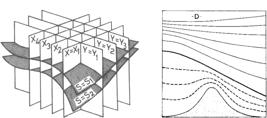
Left: Layout of (x, y, s) coordinate surfaces, reproduced from Bleck (1978a). Right: Hybrid coordinate version D, reproduced from Bleck (1978b).

The standard approach to transforming spatial derivatives from z to s space, demonstrated here for the horizontal gradient of pressure p in x,z space, is to form the total differential dp = (∂p/∂x)_z dx + (∂p/∂z)_x dz where subscripts indicate variables held constant during differentiation. Dividing this expression by dx while holding s constant, we obtain (∂p/∂x)_z = (∂p/∂x)_s − (∂p/∂z)_x (∂z/∂x)_s . Under hydrostatic conditions, where the ratio of gravitational acceleration g and specific volume α equals −∂p/∂z, this leads in the case of s = p to the familiar geopotential gradient expression α(∂p/∂x)_z = (∂gz/∂x)_p while in the case of s = α(≡ ρ ⁻¹ ) it leads to Montgomery’s formula

$\alpha {\left(\partial p/\partial x\right)}_z={\left(\partial M/\partial x\right)}_{\alpha }$ (1)

where M = gz + pα. A similar expression holds in isentropic coordinates in the atmosphere. M is most easily computed - and in fact should be computed, as explained shortly - from the hydrostatic equation in the form ∂M/∂α = p.

Other partial differentials in the dynamic equations, including local time derivatives and the divergence term in the continuity equation, are transformed to s space in similar fashion. To transform derivatives of the horizontal velocity vector v = v(x, y, s, t) in the momentum equation, for example, one starts from

$$\begin{gathered} d\mathbf{v}=(\partial \mathbf{v}/\partial x{)}_{yst}dx+(\partial \mathbf{v}/\partial y{)}_{xst}dy \\ +(\partial \mathbf{v}/\partial s{)}_{xyt}ds+(\partial \mathbf{v}/\partial t{)}_{xys}dt \end{gathered}$$ (2)

which immediately leads to an expression for d v /dt, conveniently decomposed into a local time tendency and a set of three advection terms in x, y, s space.

To convert the three-dimensional divergence term ∇ _z · v +∂w/∂z in the continuity equation from z to s space, we start by expressing the horizontal component as ∇ _z · v = ∇ _s · v − (∂ v /∂z) · ∇ _s z . (Here, ∇ is the 2-dimensional gradient operator whose subscript indicates the variable held constant during differentiation.) Transformation of the remaining term, ∂w/∂z, is slightly more complex because the vertical velocity component, in contrast to u and v, must reflect a possible movement of the s surface. Our starting point is the expression

$w\equiv dz/dt=(\partial z/\partial t{)}_s+\mathbf{v}·{\nabla }_{s}z+\dot{s}(\partial z/\partial s)$

whose z -derivative is

$$\begin{gathered} \partial w/\partial z=(\partial s/\partial z)(\partial w/\partial s) \\ =(d/dt)\log (\partial z/\partial s)+(\partial \mathbf{v}/\partial z)·{\nabla }_{s}z \\ +\partial \dot{s}/\partial s \end{gathered}$$

where $\dot{s}\equiv ds/dt$. The final step in transforming the continuity equation is to add to ∂w/∂z the remaining terms (d/dt) log ρ+∇ _z · v from the z -coordinate form of the continuity equation, making use of the expression for ∇ _z · v obtained earlier:

$$\begin{gathered} (d/dt)\log \rho +{\nabla }_z·\mathbf{v}+\partial w/\partial z= \\ (d/dt)\log (\rho \partial z/\partial s)+{\nabla }_s·\mathbf{v}+\partial \dot{s}/\partial s=0 \end{gathered}$$

The flux form of this equation under hydrostatic conditions is

$\frac{\partial }{\partial t}\left(\frac{\partial p}{\partial s}\right)+{\nabla }_s·\left(\mathbf{v}\frac{\partial p}{\partial s}\right)+\frac{\partial }{\partial s}\left(\dot{s}\frac{\partial p}{\partial s}\right)=0$ (3)

The mass continuity equation in this form is the basic building block for all tracer conservation equations in s space. Further details will be omitted here but are laid out, for example, by Kasahara (1974) and Bleck (1978a).

VERTICAL COORDINATES: σ AND z

Due to the relative absence of erosion, shelf breaks and mountain ranges on the seafloor are steeper by far than terrestrial mountains. Hence, σ coordinate surfaces tend to be more steeply inclined in basinscale ocean models than they are in atmospheric models - to the point where diagnosis of the horizontal pressure force from mass field information carried on sloping σ surfaces becomes a serious problem. For this reason, terrain-following coordinates in the ocean are mainly used in models of shelf seas [e.g. Blumberg & Mellor (1987), Shchepetkin & McWilliams (2003)]. Figure 1 (right), which we will discuss in a different context later, shows a sketch of σ coordinate representation in the lower part of a model atmosphere.

A better choice than σ in basin-scale models is the z coordinate with bottom topography approximated by cuboids of different heights. This coordinate, in which cuboid height is constrained by the model’s vertical resolution to assure that grid cells in x,y,z space are cuboid-shaped as well, has the advantage of allowing precise evaluation of the horizontal pressure force. We should mention that Mesinger et al. (2012) have introduced a similar feature in σ-coordinate weather models; their scheme allows individual σ surfaces to laterally terminate at the top of escarpments rather than being forced to climb over mountainous obstacles. The weather community has not fully embraced this elegant design, one reason being that vertical sidewalls tend to create spikes in precipitation statistics.

DENSITY AS VERTICAL COORDINATE

Oceans and atmospheres are "shallow" fluids in which horizontal motion dominates, but where vertical displacement nevertheless plays an important role in setting the vertical structure of heat and momentum fields. In the 1930s, when synoptic aerological observations became frequent enough to allow the charting of air flow in the free atmosphere, the complexities of analyzing three-dimensional flow patterns became apparent. In a seminal article, Rossby & Collaborators (1937) addressed this problem by treating the atmosphere as a stack of quasiimmiscible material layers, thereby effectively reducing a three-dimensional analysis problem to a set of two-dimensional ones. A suitable variable to associate with those layers was entropy or a variable related to it, such as buoyancy or potential temperature, given that fluid motion in the ocean and atmosphere away from boundaries can often be treated as adiabatic.

Oceanographers were quick to follow (Montgomery 1938) but had to use potential density, another variable conserved in adiabatic flow, in lieu of entropy due to the difficulty of measuring entropy in the ocean. In fact, the isentropic and isopycnic analogs of the isobaric geopotential, crucial for analyzing synoptic-scale flow patterns from sparse velocity and mass field observations, were first derived in the oceanic context (Montgomery 1937).

On the atmospheric side, an unfortunate flaw in the computation of M from radiosonde data severely complicated isentropic analysis and arguably stood in the way of its being adopted in operational meteorology. It was Danielsen (1959) who pointed out that independent evaluation of the two terms in the expression for M ignores the high degree of error cancellation between the two terms. A hydrostatic equation formulated with M as the unknown accounts for this cancellation¹.

Despite this setback, interest in simplifying the study of three-dimensional flow by utilizing a quasimaterial vertical coordinate persisted, as this would allow researchers to reduce the spatial complexity of many phenomena. Starr (1945) laid the theoretical groundwork for this type of work by formulating the dynamic equations in a material or, as he called it, quasi-Lagrangian reference frame.

One welcome attribute of a material vertical coordinate, which we will return to later, is its ability to suppress numerical diffusion of tracer fields subjected to fluctuating vertical velocities. To illustrate this, we show in Figure 2 the evolution of a hypothetical tracer lifted in the water column during one time step and lowered during the next one, as may happen during passage of an internal gravity wave. In a fixed grid, the so-called rezoning step required at the end of the first time step causes tracer material to leak into the cell above. Only a small amount of this material returns to the original cell during the following subsidence step; furthermore, rezoning now causes tracer to leak into the cell below. At the end of the second time step, tracer concentration in the original cell in this example has dropped by 32%.

Figure 2
Transport-induced vertical diffusion in (a) "level" models (models using a fixed-depth vertical coordinate) and (b) "layer" models (models using a material vertical coordinate).

The rightmost three columns in Figure 2 illustrate the obvious, namely, that without rezoning the tracer stays in the original grid cell.

The material presented in the remainder of this article is organized in a way that mirrors the historical development of isopycnic ocean models. Section 2 deals with early "process" models in rectangular basins driven by idealized wind stress fields, later extended to real ocean basins with variable bottom depth forced by realistic wind fields. The problem of applying buoyancy forcing to a model which uses buoyancy as an independent variable is dealt with in Section 3. Techniques to overcome the incompressibility assumption traditionally made in isopycnic ocean models are discussed in Section 4. The hybrid-isopycnic coordinate framework, developed to address various limitations of "pure" isopycnic models, is covered in Section 5. Transformation of gridded fields as it relates to isopycnic model initialization and post-processing is briefly discussed in Section 6. The article ends with concluding remarks in Section 7.

EARLY WIND-DRIVEN ISOPYCNIC MODELS

TWO-LAYER PROCESS MODELS

Several barriers stand in the way of widespread use of an entropy-related vertical coordinate in geophysical fluid modeling, the most important one undoubtedly being that these coordinate surfaces can intersect the upper or lower domain boundary. Coordinate surfaces that cease to exist over parts of the computational domain, or are not always nicely separated from one another, complicate the design of finite-difference operators. A number of remedies for overcoming this layer "outcrop" problem (a term borrowed from geology where it describes rock layers rising from the earth’s interior to the surface) have been developed over the years, but before these became available, applications of isopycniclayer models were restricted to scenarios where outcropping did not occur. Consequently, early isopycnic models were characterized by extremely coarse vertical resolution (typically no more than 2 layers), uniform surface density, and a bottom layer deep enough to prevent bottom topography from intersecting the lowest interior layer interface.

While these models were incapable of simulating real-world ocean circulations in great detail, they served as important tools for explaining and understanding phenomena such as western boundary currents and dynamic instabilities observed in the real ocean. Theoretical treatment of these processes typically involved oneor two-layer abstractions of the real ocean, e.g. Pedlosky (1964) and Welander (1966). Examples of process-oriented numerical simulations conducted in the two-layer framework are the works of Holland & Lin (1975a), Holland & Lin (1975b), Hurlburt & Thomson (1976), and Hurlburt & Thomson (1980). The contributions of Holland and Lin (loc.cit.) in particular set the stage for later multi-layer work.

As explained by Orlanski (1969), for example, baroclinic instability results from the interaction of two properly-positioned potential vorticity (PV) anomalies. In the classical Eady (1949) model these anomalies are provided by thermal gradients on both the upper and lower boundary, but in the atmospheric context the anomalies typically are a combination of a PV anomaly embedded in the upper troposphere and a temperature anomaly at the lower boundary [Bretherton (1966), Bleck (1990)]. Importantly, PV anomalies created by a single sloping interior interface in a 2-layer isopycnic model are able to spawn baroclinic instability. This allowed Holland & Lin (1975b) to study baroclinic instability in their simple 2-layer, flat-bottom model devoid of density anomalies at the surface or bottom.

As layers are added to an isopycnic model to increase its vertical resolution, the layer outcrop problem must sooner or later be addressed. This issue is dealt with in the following section. Still, multilayer models devoid of outcropped layers occasionally find use in theoretical investigations of geophysical fluid phenomena. An example of such work can be found in Herbette et al. (2003). Note that layer thickness - the denominator in the isopycnic rendition of Ertel’s Potential Vorticity Theorem - is a prognostic variable in “stacked shallow-water" models of the type discussed here. This makes them particularly useful for PV-oriented diagnostic work. With a bit of poetic license, we can borrow a term from biology and say that PV is important because it sits at the top of the dynamic food chain.

TREATMENT OF LAYER OUTCROPPING

Replicating or extending theoretical investigations of ocean dynamics in a 2-layer environment is enlightening but not the ultimate goal of ocean modeling. To expand the range of phenomena tractable by isopycnic ocean models, the roadblock mentioned earlier regarding the outcropping of coordinate layers quickly became the number-one issue. The course taken by modelers at the University of Miami was to extend outcropped layers as zero thickness or "massless" layers into regions where they do not physically exist, and to find numerical algorithms capable of handling the transition between masscontaining and massless portions of a coordinate layer. The massless layer concept was first introduced by Lorenz (1955); it has more recently been exploited by de Verdière et al. (2018) in their work on available potential energy in isopycnic models.

A promising algorithm for the stated task was found in the Flux-Correct Transport (FCT) scheme [Boris & Book (1973), Zalesak (1979)]. A model incorporating this scheme was first used in simulations by Bleck & Boudra (1986). This model, many of whose features were inherited from a hybridisopycnic coordinate model published a few years earlier (more on that below), consisted of four active layers in a rectangular flat-bottom basin. Unwelcome spikes in the intensity of wind forcing in a surface layer transitioning to a massless state were avoided by distributing wind stress over a fixed depth interval, assuming a linear stress profile. Bleck & Boudra (1986) compared this model to the earlier hybrid model of Bleck & Boudra (1981) and to a version reconfigured in traditional depth coordinates to shed light on the sensitivity of the solutions to different coordinates choices.

Other investigators, including Huang (1986) and Bogue et al. (1986), followed the lead of Bleck & Boudra (1986) in using the FCT algorithm, though only in models with one active layer. Other work to be mentioned in this context is the one by Sun et al. (1993) who compared FCT in a 3-layer buoyancyforced model to the MPDATA (Multidimensional Positive Definite Advection Transport Algorithm) scheme of Smolarkiewicz (1984) - an alternate and equally successful algorithm permitting partially massless layers. Only minor differences in the performance of the two schemes were found.

Another positive-definite advection scheme suitable for handling massless layers, this one developed by Hsu & Arakawa (1990) for use in an atmospheric isentropic model, was applied in an oceanic process study by Hallberg & Rhines (1996).

BAROTROPIC/BAROCLINIC MODE SEPARATION

The next step in isopycnic model design was the development of a procedure for independently timestepping the barotropic and baroclinic modes. Since barotropic gravity waves typically propagate through the ocean at least 20 times faster than other signals, numerical efficiency can greatly be increased by filtering these waves from the time-consuming layerby-layer integration of the prognostic equations. Historically, mode splitting was achieved through the so-called rigid-lid approximation (Bryan 1959), but this approach requires solving an elliptic equation for the barotropic stream function, a complex endeavor in the presence of islands.

A simple way around the numerical efficiency problem created by barotropic gravity waves is to totally eliminate the barotropic mode by making the bottom layer infinitely deep, and thus motionless. Multilayer isopycnic models belonging to this socalled reduced-gravity class have been used in work by, among others, Jensen (1991), Jensen (1993), Schopf & Loughe (1995), and Burgman et al. (2008). The Schopf & Loughe (1995) model, which was equipped to handle buoyancyin addition to windforcing, became known as the POSEIDON model.

Reduced-gravity models, i.e. models with a motionless bottom layer, are useful for studying near-surface processes but are essentially incapable of simulating the global thermohaline-driven overturning circulation or the influence of variable bathymetry on abyssal flows. For this reason, modelers at the University of Miami opted for the socalled split-explicit approach which in essence subtracts the barotropic mode from the model state at the beginning of each long (baroclinic) time step, advances the barotropic mode in a single-layer calculation using multiple short (barotropic) time steps, and adds it back at the end of the baroclinic step.

The work of Browning & Kreiss (1994) tells us that split-explicit integration schemes are a veritable breeding ground for numerical instabilities. After much experimentation, Bleck & Smith (1990) arrived at a splitting technique which, though saddled with some undesirable side effects, was sufficiently stable to hold up under the rigors of realbasin modeling. The need to dampen unstable modes in the adopted scheme by increasing lateral viscosity was avoided in their model by formulating the nonlinear terms in the momentum equation in enstrophy-conserving form and applying a heavy time smoother.

Finite-difference approximations of the shallowwater equations that are designed to conserve enstrophy (the domain integral of squared vorticity) are attractive because the built-in conservation of a squared quantity immunizes them against certain types of numerical instability. One aggravating aspect is that they require division by layer thickness, so a workaround had to be developed to cope with layers transitioning to a massless state at the sea surface or sea floor. Details can be found in Bleck & Smith (1990).

For further discussion of barotropic-baroclinic mode splitting in layer models, see Dukowicz (2006) and Higdon (2008).

One of the undesirable side effects just alluded to is that the Bleck & Smith (1990) scheme treats salinity as massless because the baroclinic part of the circulation is not allowed to change bottom pressure. Surface freshwater fluxes therefore must be applied in the form of virtual salt fluxes. This not only precludes faithful rendition of what Huang (1993) calls "natural" boundary conditions but also requires special steps to assure global salt conservation, given that salinity tends to be high [low] in regions where evaporation [precipitation] dominates.

Other numerical refinements of the model, also outlined in Bleck & Smith (1990), include a scheme for applying sidewall drag in partially blocked layers (layers whose lower interface intersects the bottom but whose upper interface does not), and a lateral extrapolation scheme for computing the horizontal pressure force in locations where a layer intersects a steep bottom slope.

Results from wind-forced simulations of the North Atlantic basin making use of the above refinements are given in Smith et al. (1990). This particular model, later equipped to allow buoyancy forcing, became known as MICOM, the Miami isopycnic coordinate ocean model. A key accomplishment at the time were truly eddy-resolving simulations [mesh size 0.08^◦ × cos(lat.)] of the North Atlantic, made possible through collaboration with computer scientists at the University of Minnesota (Bleck et al. 1995).

SURFACE BUOYANCY FORCING OF ISOPYCNIC MODELS

THE KRAUS-TURNER MODEL

While wind stress is an externally imposed forcing field which is fairly independent of the ocean state, not all buoyancy forces can be treated this way. Physical reasoning suggests that sensible and latent heat fluxes in particular should depend on differences of the pertinent variables across the air-sea interface; hence, the strength of surface buoyancy forcing is a function of ocean surface conditions.

Atmospheric temperature and moisture are typically supplied as fields varying in space and time and require matching ocean surface fields for the proper evaluation of buoyancy fluxes. However, buoyancy in an isopycnic model serves as a discretized vertical coordinate. This creates a conundrum for which no universally accepted solution has been found.

One strategy in buoyancy-forced isopycnic ocean models is to add a variable-density surface layer representing the oceanic mixed layer. This layer is then capable of properly handling turbulent airsea exchange processes along the lines of Kraus & Turner (1967) (KT for short), Niiler & Kraus (1977) and Gaspar (1988).

There is a sizable list of isopycnic model applications incorporating various renditions of the KT scheme for surface forcing. The list, most likely incomplete, includes contributions of Kraus et al. (1988), Bleck et al. (1989), Bleck et al. (1992), Oberhuber (1993), Mikhailova & Shapiro (1993), Bleck & Chassignet (1994), Schopf & Loughe (1995), New et al. (1995), Chassignet et al. (1996), Roberts et al. (1996), Bleck et al. (1997), Hallberg (1997), Hu & Chao (1999), Vigan et al. (2000), Sun & Bleck (2001), Schmid et al. (2003), Furevik et al. (2003), Wallcraft et al. (2003), and Hallberg & Gnanadesikan (2006).

Oberhuber’s model is special in that it uses (i) movable sidewalls to overcome the layer outcropping problem and (ii) an implicit scheme to advance the model state in time.

With the addition of a variable-density surface mixed layer, the isopycnic layer outcropping problem shifts from the sea surface to the bottom of the mixed layer. In this case, the location where an isopycnic layer outcrops now depends on the mixedlayer density field. To maintain stable stratification, mixed-layer density may not exceed the density of mass-containing layers below. Whenever this happens in a grid column, the mixed layer must absorb the respective layers which thereby are rendered massless.

An important process captured by the KT scheme is the annual (as well as daily) variation in mixed layer depth. When the mixed layer deepens, as happens, for example, during surface cooling, entrainment of water from layers below poses no numerical challenge. Mixed-layer shoaling, on the other hand, requires special treatment because the mixed layer cannot, due to the discrete density structure of the ocean interior, simply detrain water into the interior. Two possible strategies to deal with this issue are described below.

MIXED LAYER DETRAINMENT OPTIONS

One strategy to deal with the mixed-layer detrainment problem is to simply add the detrained water to the uppermost mass-containing isopycnic layer (Schopf & Loughe 1995) and then gradually restore its target density by entraining denser water from below. Another possibility, this one employed by Bleck et al. (1989) and Bleck et al. (1992) in MICOM, amounts to dividing the uppermost layer into an active and a "fossil" mixed layer residing underneath the active one. This fossil layer acts as a temporary receptacle for detrained mixed-layer water.

Caution must be exercised in either approach to avoid long-term trends in layer structure, i.e. excessive expansion of nonisopycnic subsurface layers. If the fossil layer scheme is used, it is important to always look for opportunities to return fossil mixed layer water to the isopycnic interior. This involves further dividing the fossil layer into two sublayers and vertically transferring density in each grid column in such a way that the top sublayer tracks the density field of the mixed layer (thereby maintaining stable stratification) while the bottom one matches the density of the uppermost interior layer. The lower sublayer so defined can then be transferred to the isopycnic layer.

The amount of water detrained this way can strongly vary, both temporally and spatially. If the mixed layer density decreases only slowly, the lower sublayer detrainable after each time step will in general be very shallow. Yet even in the case where the total fossil layer can be detrained, the overall column density structure will hardly be affected; the top interface of the entraining isopycnic layer merely moves up to the bottom of the active mixed layer. However, the resulting thickness bumps, both in the fossil layer and the interacting interior layers, may lead to undesirable lateral diffusion of layer thickness when solving the dynamic equations; this must be taken into consideration.

We will not dwell on additional complexities in the fossil-layer approach arising from the fact that in models carrying variable temperature and salinity it is difficult to achieve the correct target density when combining the lower fossil sublayer with the chosen interior layer. Suffice it to say that coordinate maintenance is a broader issue extending past mixed-layer detrainment in isopycnic models carrying both temperature and salinity as prognostic variables. Due to the nonlinearity of the equation of state for seawater, maintaining target coordinate values in this model class is most easily achieved iteratively via small interlayer mass exchange, as is done in the Schopf & Loughe (1995) scheme.

The buoyancy forcing complexities just discussed were a major driver toward the hybrid coordinate concept (see Section 5) where near-surface coordinate layers can be configured as prescribedthickness layers which seamlessly revert to isopycnic ones at depth. The hybrid coordinate approach, which among other advantages allows the KT bulk mixed layer to be replaced by more elaborate turbulent closure schemes, see Halliwell (2004) and Kara et al. (2008), will be discussed in a later section.

For a summary of MICOM’s design features, including the governing equations and additional topics such as isoand diapycnal mixing, see Bleck & Chassignet (1994). Note that coarse-mesh (i.e. non-eddy-resolving) isopycnic coordinate models allow subgrid-scale diapycnal mixing to be parameterized as lateral diffusion of isopycnic layer thickness, in line with the work of Gent & McWilliams (1990) and Drijfhout & Hazeleger (2001). In practice, this boils down to adding a mixing term to the continuity equation (Eqn. 3). The term captures the effect of baroclinic instability whose overall function in the ocean is to counteract the steepening of isopycnals by differential thermohaline forcing.

THERMOBARICITY

As pointed out at the beginning of this article, the purpose of mapping three-dimensional oceanic and atmospheric flow onto a set of isopycnic or isentropic surfaces is to simplify the dynamics by eliminating the vertical component of motion wherever the flow is adiabatic. In the atmosphere, where compressibility is constant except for minor variations due to water vapor, potential density (buoyancy) is a close proxy for entropy. Thus, not only does large-scale adiabatic flow in the atmosphere take place along isentropic surfaces, but subgrid-scale eddy mixing, which mainly takes place among fluid parcels of equal buoyancy, occurs along these surfaces as well. In other words, atmospheric adiabatic motion on both resolved and unresolved scales is confined to isentropic surfaces.

The situation is more complex in the ocean where temperature and salinity have comparable effects on buoyancy and affect compressibility in different ways. A direct result is that comparing the buoyancy of two water parcels can yield different answers depending on the reference pressure at which the comparison is made.

All isopycnic layers, even the densest ones, outcrop at least intermittently somewhere in the global domain. This is to say that a layer can potentially span the whole oceanic depth range. Thus, the option of using layer-index dependent reference pressures for potential density calculations is not available, except possibly in the subtropical warmwater sphere.

The need to settle on a global reference pressure has various implications. No matter which reference pressure is chosen, there will be oceanic regions where subgrid-scale eddy mixing is not well aligned with coordinate surfaces based on this reference pressure - or worse yet, where potential density surfaces computed from the observed temperature and salinity fields will fold.

The latter issue is of particular concern in locations like the Southern Ocean where successful simulation of seasonal ice coverage requires maintenance of the summertime meltwater cap and accurate rendition of vertical heat fluxes. These processes will be affected if the model falsely initiates convective adjustment to remove misdiagnosed static instabilities. An inappropriate reference pressure can also render the water in the lower branch of the Atlantic meridional overturning circulation too light and thus subject to convective mixing (Lynn & Reid 1968).

Eddy mixing predominantly takes place along buoyancy-neutral surfaces (McDougall 1987). The orientation of a neutral surface is defined locally by its normal vector β∇S − α∇θ, where S, θ are salinity and potential temperature, and α, β are the thermal expansion and saline contraction coefficients, respectively. As Jackett & McDougall (1997) explain, the local planes so defined can be extended into a well-defined global surface only if, after multiplication by an integrating factor if needed, the normal vector can be expressed as the gradient of a single scalar function. This condition would be satisfied if α, β were constants, but since both are functions of S, θ, and pressure p, this integrability condition is only approximately satisfied. Jackett & McDougall (1997) developed an algorithm for finding global surfaces that are close to neutral, but their algorithm is an iterative one which appears to be too complex for time-dependent ocean modeling.

VIRTUAL POTENTIAL DENSITY

Sun et al. (1999) (S99 hereafter) proposed a scheme that goes a long way toward solving the problem of (θ, S)-dependent sea water compressibility. Recall that potential density ρ_pot is the vertical coordinate of choice because this variable is conserved in adiabatic flow. Traditional isopycnic models go one step further: they not only define their vertical grid in terms of ρ _pot but also assume water in each coordinate layer to have a density equal to the ρ _pot value assigned to that particular layer. This is to say that they do not distinguish between in-situ and potential density. Sea water is thereby rendered incompressible, though the layer density so defined is by choice layer-dependent. The reason for this particular treatment is clear when retracing the steps leading to Eqn. 1: A hydrostatic equation of the form ∂M/∂α _pot = p (where α _pot = 1/ρ _pot ) allows the horizontal pressure gradient in the momentum equation to retain its singleterm form, namely, the isopycnic gradient of Montgomery potential M = gz + pα _pot .

The crucial step taken by S99 is to sever the connection between the definition of coordinate layers and the buoyancy properties of the water residing inside them. However, allowing layer density to deviate from ρ _pot spawns a second term on the right-hand side of Eqn. 1. Replacing the variable α _pot by an as yet undefined variable α ^′ in both the hydrostatic equation and the pressure force term converts Eqn. 1 into

$\alpha \text{'}{\left(\frac{\partial p}{\partial x}\right)}_z={\left(\frac{\partial (gz+p\alpha \text{'})}{\partial x}\right)}_{{\alpha }_{pot}}-p{\left(\frac{\partial \alpha \text{'}}{\partial x}\right)}_{{\alpha }_{pot}}$ (4)

with an analogous expression for the y component. The extra term on the right-hand side involves the isopycnal gradient of whichever variable replaces potential specific volume in the coordinate layers. The goal of S99 is to find a buoyancy variable that retains compressibility effects yet avoids making the last term in Eqn. 4 in steeply inclined isopycnic layers as large as it would be, for example, if in-situ specific volume were the variable of choice for α ^′ .

S99 achieves this goal by defining a new variable called "virtual" potential density which is numerically close to regular potential density but retains information about the effect of θ, S variations on the buoyancy in each layer.

Virtual potential density is obtained by splitting sea water compressibility into a purely p-dependent component and a residual "thermobaric" component which is primarily a function of θ and S. Compression caused by the former, though much larger than the latter in the relevant θ, S range, is dynamically irrelevant. Hence, removing from the in-situ density the compression effect of the purely p-dependent component of compressibility will have no dynamic consequences while serving the purpose of producing a density field rather similar to regular potential density. A different way of saying this is that virtual potential density is computed by using constant (but representative) values of θ, S in the compressibility formula when moving a parcel to its chosen reference pressure.

S99 demonstrates the capabilities of their approach by reproducing the double reversal with depth of the interhemispheric meridional pressure force responsible for the alternating flow direction in the Atlantic - northward at top and bottom, southward in between. This double reversal cannot be achieved in the traditional incompressible isopycnic framework.

THE CONTACT-PRESSURE INTEGRAL

Hallberg (2005) has been able to isolate a numerical instability related to the treatment of thermobaricity in layered ocean models. The instability is caused by the second term in the pressure gradient formula(Eqn. 4) whose partial suppression is the aim of S99. Since thermobaricity-related instabilities do occasionally surface in fine-mesh HYCOM² applications [e.g. Arbic et al. (2018)], the search continues for a reliable algorithm for numerically evaluating the horizontal pressure gradient force in the challenging situation where density varies laterally in steeply inclined coordinate layers.

A compelling alternative to the S99 treatment has been presented by Adcroft et al. (2008). Their approach, which builds upon Lin (1997) and Shchepetkin & McWilliams (2003), is to replace the ordinary finite-difference pressure gradient expression by a numerically precise evaluation of the net contact pressure on the six faces of each grid cell. In the name of accuracy they not only evaluate the vertical legs of the contact pressure integral in exact form by using an integrable equation of state, but they also replace the standard logarithm function in the computer library by a more accurate version. Together, these steps allow them to use in-situ density as the buoyancy-controlling variable - precisely the choice causing instability when approximating the horizontal pressure gradient by a standard two-term finite-difference formula.

Attempts to implement the Adcroft et al. (2008) approach in HYCOM have failed so far. Possible reasons include the use of a standard singleprecision version of the log function, as well as subtle differences in the evaluation of the surface integral around grid cells truncated by bottom topography. One potential remedy is to combine the Adcroft et al. (2008) approach with S99, i.e., replace in-situ density by virtual potential density when evaluating the contact pressure integral. To our knowledge, this option is yet to be explored.

We should mention again that the vertical coordinate in HYCOM continues to be regular potential density. This variable, diagnosed independently of virtual potential density, still controls the algorithm maintaining isopycnic conditions in individual coordinate layers. (Recall that such an algorithm is needed because independently advected temperature and salinity do not always combine to yield the correct "target" potential density.)

The main reason for not switching to virtual potential density as vertical coordinate is that the latter, in contrast to potential density, is not conserved in adiabatic flow; hence, its isosurfaces are not material in adiabatic flow. The ability to relate the vertical velocity component $\dot{s}$ to diabatic processes is na advantage of the isopycnic system worth retaining.

The S99 scheme has been in use in MICOM and HYCOM for both ocean-only and coupled oceanatmosphere simulations. Examples of the former are Sun & Bleck (2001), Chassignet et al. (2003), Sun & Bleck (2006a), Cheng et al. (2007), Kara et al. (2010), Bozec et al. (2011), Le Henaff et al. (2012), Haza et al. (2012), Mensa et al. (2013), Xu et al. (2016), Chassignet & Xu (2017), Xu et al. (2018), and Chassignet et al. (2020). For examples of the latter, see Furevik et al. (2003), Cheng et al. (2004), Cheng & Rhines (2004), Bentsen et al. (2004), Bleck (2005), Sun & Bleck (2006b), Ottera et al. (2009), Megann et al. (2010), Romanou et al. (2013), Gabioux et al. (2013), Kim et al. (2014), Sun et al. (2018), Miller & Coauthors (2020), and Barton et al. (2021).

TRANSITION TO HYBRID COORDINATES

To trace the history of hybrid coordinates we need to go back to Bleck (1978b) who compared the performance of various combinations of terrain-following and isentropic coordinates in the atmosphere. His version D, which uses an especially compelling blend of the two coordinates and is illustrated here in Figure 1 (right), may be viewed as the ancestor of "hybrid"-coordinate ocean models, hybrid defined here as a blend of density and prescribed-depth coordinates. An early ocean model encompassing this concept was developed by Bleck & Boudra (1981). Their 4-layer wind-forced box model, built before the layer outcrop problem was solved, used hybridization essentially as a safety valve to keep the uppermost interior layer interface from rising to the sea surface under the influence of cyclonic wind stress. The model was shelved when positivedefinite transport schemes like FCT and MPDATA became available (Bleck & Boudra 1986), only to be resurrected when complications with buoyancy forcing began to stand in the way of wider use of isopycnic models.

The hybrid coordinate concept was further formalized by Bleck (2002), yielding a MICOM-based model named HYCOM. A simple formula comprising the essence of hybrid coordinate design is

$\left(\begin{array}{c}\mathrm{vertical}\\ \mathrm{motion}\\ \mathrm{OF}\\ \mathrm{layer}\\ \mathrm{interface}\end{array}\right)+\left(\begin{array}{c}\mathrm{vertical}\\ \mathrm{motion}\\ \mathrm{THROUGH}\\ \mathrm{layer}\\ \mathrm{interface}\end{array}\right)=\left(\begin{array}{c}\mathrm{vertically}\\ \mathrm{integrated}\\ \mathrm{horizontal}\\ \mathrm{mass}\mathrm{flux}\\ \mathrm{divergence}\end{array}\right)$ (5)

This equation makes use of the well-known fact that hydrostatic models diagnose the vertical material motion dp/dt from the layer-discretized form of the continuity equation (Eqn. 3), specifically from the vertically integrated layerwise mass flux divergence. It furthermore makes the almost trivial statement that the physical vertical motion so obtained can be divided into motion of a coordinate surface and motion relative to it. Note that Eqn. 5 covers the extreme cases of a fixed grid (zero first term on the left), a material vertical coordinate (zero second term on the left), and everything in-between.

UNSTRUCTURED (FREE-FORM) HYBRIDIZATION

Eqn. 5 empowers the model architect to decide where in a grid column to place individual grid points - resting or moving - and to solve for the coordinatespecific vertical velocity component consistent with that placement. An analytic formula specifying the location of a grid point in p space as a function of, say, bottom pressure, potential density, or layer index is not required.

Hybrid-coordinate models have one additional time-dependent variable not found in traditional fixed-grid models, namely, coordinate layer thickness. Therefore, one additional equation is needed in the set of model equations. This equation basically is a prescription for how to divide the quantity on the right-hand side of Eqn. 5 among the two terms on the left. It is commonly called the grid generator.

One of the duties of the grid generator is to prevent the occurrence of massless layers in the upper ocean, which can be accomplished by prescribing a minimum layer thickness typically chosen to be layer-index dependent. The algorithm should also be equipped to smooth out the transition between subdomains where interfaces follow isopycnals and subdomains (typically near the sea surface) where interfaces are depth-constrained. This can be accomplished, for example, by reducing layer-to-layer thickness contrasts in the transition region. [For a rudimentary attempt to accomplish the latter, see Appendix C of Bleck & Boudra (1981)]. For numerical efficiency reasons, the grid generator should be designed to operate on each grid column separately, i.e. should not have to look sideways at neighboring columns.

Hybrid-coordinate models are members of the ALE model class, where ALE stands for arbitrary Langrangian-Eulerian (Hirt et al. 1974). The ALE approach was originally developed for initial-value problems, so its use in geophysical fluid modeling required development of methods to maintain the overall balance between Eulerian and Lagrangian grid representation in long-term model runs. To maintain this balance, the grid generator must include a mechanism to restore the isopycnic character of coordinate layers wherever this can be achieved without violating minimum-thickness constraints. Details of such a grid maintenance algorithm are described in Bleck (2002), Halliwell (2004), Bleck (2006), and Adcroft et al. (2019).

For related work on introducing a generalized vertical coordinate into a lake model, in this case as a flexible generalization of a terrain-following coordinate, see Zhang et al. (2015).

FORMULA-GUIDED HYBRIDIZATION

An alternative approach to generalized-coordinate modeling, mainly pursued in the meteorological community, should be mentioned here. Zhu et al. (1992), Zhu & Schneider (1997), Konor & Arakawa (1997), Johnson & Yuan (1998), Webster et al. (1999), Mahowald et al. (2002) (and possibly others) avoid coordinate intersection problems in their isentropic models by defining coordinate surfaces as F (θ, σ, p) = const. where the function F is constructed so as to approach the terrain-following coordinate σ near the ground, potential temperature θ in the free atmosphere, and (optionally) pressure p near the model top. Various alternatives are proposed for F with the goal of maximizing the grid space occupied by purely isentropic surfaces while smoothing the transition between the σ, θ, p domains and, importantly, avoiding the problem of coordinate surface entangling. Version D of the four alternatives considered by Bleck (1978b), illustrated in Figure 1 (right), falls into this model class.

While the availability of an analytic formula for an intersection-free hybrid vertical coordinate offers advantages in terms of both elegance and ease of documentation, a formula robust enough to hold up everywhere in the global ocean or atmosphere imposes restrictions which are circumvented by the free-form grid-generator approach advocated by Bleck (2002).

A brief remark regarding the expression "free form" is in order. The Bleck (1978b) paradigm does not require the vertical coordinate s to be defined in mathematical or physical terms. In particular, s does not have to be differentiable with respect to height or pressure. This requires that the governing equations can be written in a form where (i) partial derivatives with respect to s are eliminated (with the exception of ∂p/∂s whose finite-difference analog represents layer thickness) and (ii) the potentially meaningless quantity $\dot{s}\equiv ds/dt$ is multiplied wherever it occurs by ∂p/∂s. The purpose of (ii) is to produce a physically meaningful vertical velocity component, dimensioned pressure/time, which is independent of the meaning of s. The fused product $(\dot{s}\partial p/\partial s)$ so created is easily recognized as the vertical motion referred to in the second term in Eqn. 5. There never is any reason to break it up into its two components.

Requirements (i) and (ii) can be met simultaneously by multiplying and dividing nonconforming terms in the governing equations by ∂p/∂s. The vertical advection term (∂ v /∂s)ds in Eqn. (2), for example, can be written in light of $ds=\dot{s}dt$ as

$\frac{\partial \mathbf{v}}{\partial p}\left[\dot{s}\frac{\partial p}{\partial s}\right]dt$

which satisfies both (i) and (ii). Evaluating the vertical advection term written in this form, with $(\dot{s}\partial p/\partial s)$ supplied by the second term in Eqn. 5, is straightforward. Solving Eqn. 5 is often called the regridding step, followed by a remapping step in which the prognostic variable in question is interpolated from the old to the new grid. In the parlance of ALE, the two-step process, also illustrated in Figure 2, is referred to as rezoning (Hirt et al. 1974).

The effort of Cummings (2005), Chassignet et al. (2007) and Srinivasan et al. (2011), among others, to develop a data assimilation system for HYCOM has cemented the model’s role as a dependable provider of real-time, global fields at horizontal resolutions as high as 1/25⁰ for use in ocean research and as boundary conditions for regional models [e.g. Hurlburt et al. (2008), Zamudio & Hogan (2008), Kourafalou et al. (2009), Chassignet et al. (2009), Hansen et al. (2010), Jia et al. (2011), Shay et al. (2011), Halo et al. (2014), Metzger et al. (2014), Hurlburt et al. (2015), Hewitt et al. (2022), Zhang & Xue (2022), Zhang et al. (2023) ]. At the time of this writing, the website https://www.hycom.org/ lists 148 HYCOM-related publications during the period 2001 - 2016. The introduction of tides into HYCOM is discussed by Arbic et al. (2010). A few randomly chosen examples of work benefitting from the availability of HYCOM products, in the U.S. and elsewhere, are Jensen et al. (2016), Meza-Padilla et al. (2019), deVos et al. (2021), Pata et al. (2021), Brown et al. (2022), Roberts et al. (2022), and Sooknanan & Hosein (2022). For references to the use of MICOM and HYCOM in coupled ocean-atmosphere modeling, see Bentsen et al. (2013), Schmidt et al. (2014), and Sun et al. (2018). Real-time HYCOMbased fine-mesh ocean analyses and forecasts are currently distributed by the U.S. Navy (https://www7320.nrlssc.navy.mil/dynamic/gofs/gofs.php) and NOAA (https://polar.ncep.noaa.gov/global/).

A question arising during offline work with archived model fields, particularly when attempting to construct trajectories for tracer transport, concerns the availability of the genuine vertical velocity in the moving ALE grid. As pointed out earlier, this quantity can be obtained from the right-hand side of Eqn. 5 which under hydrostatic conditions yields the material vertical velocity dp/dt in s space. When mapping the velocity vector (u, v, dp/dt) to a fixed grid in p or z space, it is important to note that u and v represent layer averages typically assigned to layer mid-depth while dp/dt is defined on interfaces.

Offline transport of a field representing a tracer density (exotic example: lobster larvae per kg of water) is impractical, because doing so conservatively requires solving a transport equation analogous to the conservation equations for temperature and salinity. Performing this procedure offline would require archiving all three mass fluxes and layer thickness, i.e., the complete set of fields used in the model to solve the continuity equation (Eqn. 3). Note that conservation cannot be built into a trajectory-based transport scheme.

MODEL INITIALIZATION

One topic that has not been covered so far is the preparation of initial conditions for models framed in isopycnic coordinates. Depending on the source of the required data, this often involves more than simple vertical interpolation because mass field variables in a numerical model typically represent averages over coordinate layers. The implied stairstep shape of vertical profiles complicates the task of preserving column integrals during interpolation, especially if both "input" and "output" profiles (not just one of the two) are stairstep functions.

Technical aspects of transforming data between physical and model space for isopycnic model initialization, as well as for rendering output fields for postprocessing, are discussed in Bleck (1984), Appendix D of Bleck (2002), Griffies et al. (2020), In the special case of the buoyancy variable used as vertical coordinate, the crux of this transformation is a swap of dependent and independent variables, specifically between potential density as a function of pressure and pressure as a function of potential density. The Bleck (1984) procedure aims to improve the accuracy of this swap in situations where the input profile is a stairstep function. It converts a piecewise constant profile into a continuous, piecewise linear profile, as illustrated in Figure 3. The continuous curve, shown in red, is the outcome of a constrained least-squares fit which preserves the column integral taken over the input profile (shown in black) while minimizing kinks in the curve. Conversion of the curve into another stairstep profile, if needed, is straightforward. A stairstep profile whose "risers" are at prescribed locations on the abscissa is shown in green.

Figure 3
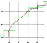
Illustration of vertical regridding, taken from a random grid location in an atmospheric model run. Black: original distribution of potential temperature (abscissa, K) as a function of pressure (ordinate, hPa). Red: piecewise linear curve fit based on Bleck (1984). Green: New stairsteps adhering to prescribed potential temperature target values 334K, 346K, 350K, etc.

CONCLUDING REMARKS

In this article we have attempted to explain the motivation for modeling the oceanic circulation in a vertically quasi-Lagrangian framework and have traced isopycnic model development from its initial stage of two-layer process studies to full-fledged general circulation modeling.

Numerical problems requiring attention as isopycnic modeling gained ground on traditional fixedgrid models included, first and foremost, the layer outcrop problem. Once numerically stable solutions to that problem were found, emphasis shifted to the complexities of applying buoyancy forcing at the sea surface. The confounding issue here is that buoyancy, a variable set by two continuously varying, boundary-forced fields (temperature and salinity), plays a double role as vertical coordinate where it is discretized into a finite set of fixed values.

Modelers eventually learned to deal with the complexities of buoyancy’s double role. Nevertheless, while the numerical schemes developed to cope with layer outcropping and buoyancy forcing passed numerical stability tests, other more subtle issues remained, such as the conservation properties of the nonlinear terms in the momentum equation and certain physical restrictions inherent in the bulk mixed layer models used to handle surface buoyancy forcing.

It became clear in the end that the pure isopycnic approach had to be modified to address the issues just mentioned. The compromise gaining ground at that time was the hybrid-isopycnic modeling framework which sacrifices the material layer concept in the near-surface ocean in favor of a prescribed vertical grid but gradually nudges the grid toward isopycnic layer representation further down in the water column where layer outcropping and mixed layer processes are no longer an issue. The main strength of the hybrid-isopycnic model is the inherent simplicity and flexibility of the grid generation process.

The impetus for engaging in isopycnic modeling has slightly shifted over the years. At the beginning, the primary motivation was to build a bridge between numerical modeling and both geophysical fluid dynamics and hydrographic research of the type conducted, for example, by Lynn & Reid (1968), Worthington (1981), and many others.

There also was - and still is - the promise of numerical efficiency gain in simulating frontal discontinuities. With fronts for dynamic reasons typically aligned with isopycnals, they manifest themselves in an isopycnic grid as geographically wide regions of small layer thickness. Thus, fine horizontal resolution to resolve fronts ceases to be an issue because their existence is encoded in the vertical grid where they expand into large-scale features. [This expansion is illustrated, for example, in Figure 7.10 in the Dutton (1976) textbook.] The above argument carries over to the simulation of quasi-circular front-like structures in ocean eddies.

A topic that came to the forefront in later years is the prevention of what has become known as the Veronis effect [ Veronis (1973), Lazar et al. (1999)]. To the extent that isopycnic surfaces resemble buoyancy-neutral surfaces, the numericallyinduced lateral leakage of properties across frontal surfaces diagnosed by Veronis (loc.cit.) is greatly suppressed in an isopycnic model. However, numerical refinements based on mixing-tensor rotation [Redi (1982), Griffies et al. (1998), Shao et al. (2020)] have reduced the severity of this problem in depth-coordinate models. The same can be said for the treatment of dense bottom water overflows (Legg et al. 2006) which are particularly easy to simulate in an isopycnic coordinate framework.

One variation on the hybrid coordinate theme we need to mention is the technique of Lin (2004) and of Leclair & Madec (2011) who aim to reduce vertical diffusion in fixed grids resulting from frequent sign changes in the vertical velocity field caused, for example, by internal gravity waves. These authors suppress the diluting effect of alternating vertical mass exchange between adjacent grid cells, illustrated in Figure 2, by treating coordinate surfaces as material during a number of time steps before restoring them to their original location. From the perspective of Eqn. 5, this entails setting the second term on the left-hand side to zero for several consecutive time steps, followed by a single step where the first term in Eqn. 5 reflects the process of grid restoration while the second term - the unknown in this case - yields the accumulated vertical transport velocity.

One important aspect of modeling fluid flow is the simulation of dynamic instabilities on meshes that are too coarse to explicitly resolve the accompanying vortex rollup process. It is worth mentioning here that the overall effect of baroclinic instability, namely, reduction of the horizontal buoyancy contrast, can be simulated in coarse-mesh isopycnic models through the addition of a lateral layerthickness diffusion term in the continuity equation (Eqn. 3). This diffusive mass flux in an isopycnic reference frame is often referred to as peristaltic or bolus flux (Dukowicz & Greatbatch 1999).

Needless to say, the ease of simulating neutralsurface mixing and baroclinic instability is sacrificed in regions where isopycnic layers are replaced by fixed-depth layers. This is one of the compromises one has to accept when engaging in hybridisopycnic modeling.

Inclusion of sea water compressibility was the last stepping stone toward full-fledged global ocean modeling in an isopycnic reference frame. The issue here is the difficulty of diagnosing the horizontal pressure force from data carried on steeply inclined coordinate surfaces. Fortuitously, this problem does not arise if water in isopycnic layers is treated as incompressible, but neglecting compressibility (in particular thermobaricity) has undesirable consequences in neutrally stratified or convectively unstable water columns. Techniques for removing the incompressibility assumption from isopycnic models are available today.

A summary of the tradeoffs between isopycnic and depth-coordinate global ocean models, as well as additional references, can be found in Griffies et al. (2010). These tradeoffs are also discussed by Willebrand et al. (2001) in a triple model study involving MICOM. An intercomparison of four oceanic general circulation models carried out by Chassignet et al. (2020) confirms HYCOM’s standing among its peers as a mature, well-performing circulation model. Recent work by Leclair & Madec (2011), Petersen et al. (2015), and Adcroft et al. (2019) indicates that the vertical ALE coordinate, though not necessarily in HYCOM’s isopycnic incarnation, is increasingly finding its way into other ocean models.

A word of caution: wholesale conversion of ocean models to an ALE coordinate, especially the isopycnic kind, might turn out to be a double-edged sword. As ocean ensemble forecasting gains traction (Thoppil et al. 2021), it is important to avoid "inbreeding" of models, especially when the ensemble concept is broadened toward multimodel ensembles, an approach already popular in climate and seasonal weather prediction. To reap the full benefits of ensemble prediction, the range of forecasts produced by individual ensemble members must be wide enough to include the actually observed evolution of the system. From this point of view, fostering differences in model numerics is undoubtedly beneficial. Concern about model genetic diversity has historically been one reason for engaging in isopycnic ocean modeling as a counterweight to traditional z -coordinate modeling.

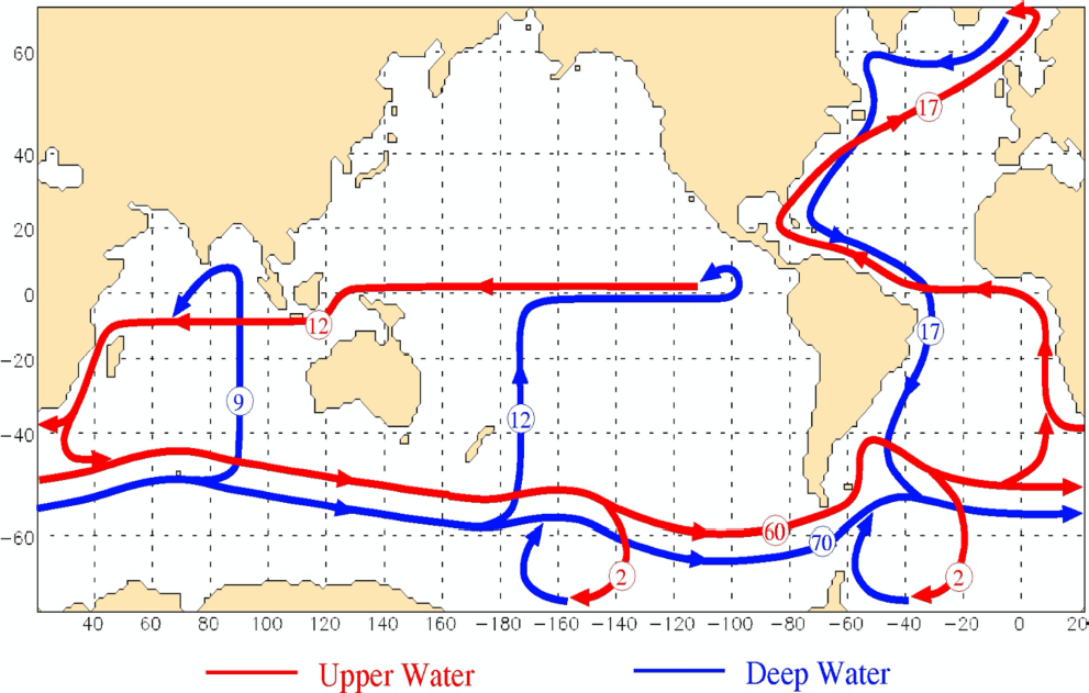
We wish to close by showing a product that illustrates ways in which isopycnic model output can be used to verify observation-based notions about the global thermohaline circulation. The stylized current threads pictured in Figure 4 were constructed by first diagnosing multi-year averages of diapycnal mass fluxes across a mid-depth isopycnal interface. This involved vertically summing up the divergence of the isopycnal mass flux above and below the chosen interface in each grid column, followed by use of Eqn. 5. Diapycnal fluxes of the same sign in contiguous geographic regions were subsequently summed up, resulting in regional totals of water mass conversion. Next, isopycnal mass flux components of the same sign were combined into bundles depicting regional totals of zonal and meridional horizontal mass flux. The bundles so obtained were subsequently simplified by removing intra-basin recirculation cells.

Figure 4
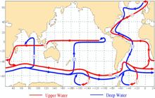
Simplified schematic of the “deep” global thermohaline circulation in the isopycnal ocean model of Sun & Bleck (2001), in a format inspired by Broecker (1991) and Schmitz (1995). Circled numbers represent transport in Sv (1 Sv = 10⁶ m ³ s ⁻¹ ). Reproduced from Sun & Bleck (2006a).

The threads shown in Figure 4 represent the end product of the above simplification process. They bear a strong quantitative relationship to observation-based illustrations by Broecker (1991) and Schmitz (1995), suggesting that isopycnic coordinate models are capable of arriving at a credible rendition of the global thermohaline-forced circulation. (Many details, such as the double reversal with depth of the meridional transport in the Atlantic mentioned earlier, obviously remain hidden in a two-layer breakdown.)

The particular model which Figure 4 is based on is the thermobarically active version of MICOM, a model choice motivated by the desire to maximize the purely isopycnic coordinate domain. Transports represent 100-yr averages from a multi-century model run driven by Coordinated Ocean-ice Reference Experiments (CORE) atmospheric forcing fields. More elaborate graphs of this type, based on a more detailed 4-layer breakdown of the world ocean mimicking Schmitz (1995), can be found in Sun & Bleck (2001).

ACKNOWLEDGMENTS

MICOM and HYCOM development has been supported over many years - in vaguely chronological order - by the following U.S. agencies: National Science Foundation, Office of Naval Research, Department of Energy, National Aeronautics and Space Administration, National Oceanic and Atmospheric Administration. Mainframe computer support in particular was provided over the years by NSF, DOE, NASA, and NOAA. The writing of this article was supported in part by the NOAA Cooperative Agreement with CIRES, NA17OAR4320101.

REFERENCES

• ADCROFT, A., ANDERSON, W., BALAJI, V., BLANTON, C., BUSHUK, M., DUFOUR, C. O., DUNNE, J. P., GRIFFIES, S. M., HALLBERG, R., HARRISON, M. J., HELD, I. M., JANSEN, M. F., JOHN, J. G., KRASTING, J. P., LANGENHORST, A. R., LEGG, S., LIANG, Z., MCHUGH, C., RADHAKRISHNAN, A., REICHL, B. G., ROSATI, T., SAMUELS, B. L., SHAO, A., STOUFFER, R., WINTON, M., WITTENBERG, A. T., XIANG, B., ZADEH, N. & ZHANG, R. 2019. The GFDL global ocean and sea ice model OM4.0: Model description and simulation features, J. Adv. Mod. Earth Syst. 11, 3167-3211. DOI: 10.1029/2019MS001726.
  » https://doi.org/10.1029/2019MS001726
• ADCROFT, A., HALLBERG, R. & HARRISON, M. 2008. A finite volume discretization of the pressure gradient force using analytic integration, Ocean Mod. 22, 106-113. DOI: 10.1016/J.OCEMOD.2008.02.001.
  » https://doi.org/10.1016/J.OCEMOD.2008.02.001
• ARBIC, B. K., ALFORD, M. H., ANSONG, J. K., BUIJSMAN, M. C., CIOTTI, R. B., FARRAR, J. T., HALLBERG, R. W., HENZE, C. E., HILL, C. N., LUECKE, C. A., MENEMENLIS, D., METZGER, E. J., MüLLER, M., NELSON, A. D., NELSON, B. C., NGODOCK, H. E., PONTE, R. M., RICHMAN, J. G., SAVAGE, A. C., SCOTT, R. B., SHRIVER, J. F., SIMMONS, H. L., SOUOPGUI, I., TIMKO, P. G., WALLCRAFT, A. J., ZAMUDIO, L. & ZHAO, Z. 2018. A primer on global internal tide and internal gravity wave continuum modeling in HYCOM and MITgcm, in E. Chassignet, A. Pascual, J. Tintoré & J. Verron (eds), New Frontiers in Operational Oceanography, GODAE OceanView, 307-392. DOI: 10.17125/gov2018.ch13.
  » https://doi.org/10.17125/gov2018.ch13
• ARBIC, B. K., WALLCRAFT, A. J. & METZGER, E. J. 2010. Concurrent simulation of the eddying general circulation and tides in a global ocean model, Ocean Mod. 32, 175-187. DOI: 10.1016/J.OCEMOD.2010.01.007.
  » https://doi.org/10.1016/J.OCEMOD.2010.01.007
• BARTON, N., METZGER, E. J., REYNOLDS, C. A., RUSTON, B., ROWLEY, C., SMEDSTAD, O. M., RIDOUT, J. A., WALLCRAFT, A., FROLOV, S., HOGAN, P., JANIGA, M. A., SHRIVER, J. F., MCLAY, J., THOPPIL, P., HUANG, A., CRAWFORD, W., WHITCOMB, T., BISHOP, C. H., ZAMUDIO, L. & PHELPS, M. 2021. The Navy’s earth system prediction capability: a new global coupled atmosphere-ocean-sea ice prediction system designed for daily to subseasonal forecasting, Earth and Space Sci. 8, 28pp. DOI: 10.1029/2020EA001199.
  » https://doi.org/10.1029/2020EA001199
• BENTSEN, M., BETHKE, I., DEBERNARD, J. B., IVERSEN, T., KIRKEVÅG, A., SELAND, O., DRANGE, H., ROELANDT, C., SEIERSTAD, I. A., HOOSE, C. & KRISTJANSSON, J. E. 2013. The Norwegian Earth System Model, NorESM1-M - Part 1: description and basic evaluation of the physical climate, Geosci. Mod. Dev. 6, 687-720. DOI: 10.5194/gmd-6-687-2013.
  » https://doi.org/10.5194/gmd-6-687-2013
• BENTSEN, M., DRANGE, H., FUREVIK, T. & ZHOU, T. 2004. Simulated variability of the Atlantic meridional overturning circulation, Climate Dyn. 22, 701-720. DOI: 10.1007/s00382004-0397-x.
  » https://doi.org/10.1007/s00382004-0397-x
• BLECK, R. 1978a. Finite difference equations in generalized vertical coordinates. Part I: Total energy conservation, Beitr. Phys. Atm. 51, 360-372.
• BLECK, R. 1978b. On the use of hybrid vertical coordinates in numerical weather prediction models, Mon. Wea. Rev. 106, 1233-1244. DOI: 10.1175/1520-0493(1978)106<1233:OTUOHV>2.0.CO;2.
  » https://doi.org/10.1175/1520-0493(1978)106<1233:OTUOHV>2.0.CO;2
• BLECK, R. 1984. Vertical coordinate transformation of vertically-discretized atmospheric fields, Mon. Wea. Rev. 112, 2535-2539. DOI: 10.1175/1520-0493(1984)112<2535:NAC>2.0.CO;2.
  » https://doi.org/10.1175/1520-0493(1984)112<2535:NAC>2.0.CO;2
• BLECK, R. 1990. Depiction of upper/lower vortex interaction associated with extratropical cyclogenesis, Mon. Wea. Rev. 118, 573-585. DOI: 10.1175/1520-0493(1990)118<0573:DOUVIA>2.0.CO;2.
  » https://doi.org/10.1175/1520-0493(1990)118<0573:DOUVIA>2.0.CO;2
• BLECK, R. 2002. An oceanic general circulation model framed in hybrid isopycnic-cartesian coordinates, Ocean Mod. 4, 55-88. DOI: 10.1016/S1463-5003(01)00012-9.
  » https://doi.org/10.1016/S1463-5003(01)00012-9
• BLECK, R. 2005. Uncertainties in climate prediction the ocean perspective, Science-Based Prediction for Complex Systems, Vol. 29, Los Alamos Science, Los Alamos Nat’l. Lab., 42-55.
• BLECK, R. 2006. On the use of hybrid vertical coordinates in ocean circulation modeling, in E. P. Chassignet & J. Verron (eds), Ocean weather forecasting, Springer, 109-126.
• BLECK, R., DEAN, S., O’KEEFE, M. & SAWDEY, A. 1995. A comparison of data-parallel and message-passing versions of the Miami Isopycnic Coordinate Ocean Model (MICOM), Paral. Comput. 21, 1695-1720. DOI: 10.1016/0167-8191(95)00043-3.
  » https://doi.org/10.1016/0167-8191(95)00043-3
• BLECK, R., HANSON, H. P., HU, D. & KRAUS, E. B. 1989. Mixed layer-thermocline interaction in a three-dimensional isopycnic coordinate model, J. Phys. Ocean. 19, 1417-1439. DOI: 10.1175/1520-0485(1989)019<1417:mltiia>2.0.co;2.
  » https://doi.org/10.1175/1520-0485(1989)019<1417:mltiia>2.0.co;2
• BLECK, R. & BOUDRA, D. B. 1981. Initial testing of a numerical ocean circulation model using a hybrid (quasiisopycnic) vertical coordinate, J. Phys. Ocean. 11, 755-770. DOI: 10.1175/15200485(1981)011<0755:ITOANO>2.0.CO;2.
  » https://doi.org/10.1175/15200485(1981)011<0755:ITOANO>2.0.CO;2
• BLECK, R. & BOUDRA, D. B. 1986. Wind-driven spin-up in eddy-resolving ocean models formulated in isopycnic and isobaric coordinates, J. Geophys. Res. 91C, 7611-7621. DOI: 10.1029/JC091IC06P07611.
  » https://doi.org/10.1029/JC091IC06P07611
• BLECK, R. & CHASSIGNET, E. 1994. Simulating the oceanic circulation with isopycniccoordinate models, in S. K. Majumdar (ed.), The Oceans: Physical-Chemical Dynamics and Human Impact, Pennsylvania Acad. of Sci., 17-39.
• BLECK, R. & SMITH, L. 1990. A wind-driven isopycnic coordinate model of the North and Equatorial Atlantic Ocean. 1. model development and supporting experiments, J. Geophys. Res. 95C, 3273-3285. DOI: 10.1029/jc095ic03p03273.
  » https://doi.org/10.1029/jc095ic03p03273
• BLECK, R., ROOTH, C., HU, D. & SMITH, L. T. 1992. Salinity-driven thermocline transients in a windand thermohaline-forced isopycnic coordinate model of the North Atlantic, J. Phys. Ocean. 12, 1486-1505. DOI: 10.1175/15200485(1992)022<1486:sdttia>2.0.co;2.
  » https://doi.org/10.1175/15200485(1992)022<1486:sdttia>2.0.co;2
• BLECK, R., SUN, S. & DEAN, S. 1997. Global ocean simulations with an isopycnic coordinate model, Some new directions in science on computers, World Scientific, 297-317.
• BLUMBERG, A. & MELLOR, G. L. 1987. A description of a three-dimensional coastal ocean circulation model, in N. S. Heaps (ed.), Three-dimensional coastal ocean models, Amer. Geophys. Union, 1-16. DOI: 10.1029/co004p0001.
  » https://doi.org/10.1029/co004p0001
• BOGUE, N. M., HUANG, R. X. & BRYAN, K. 1986. Verification experiments with an isopycnal coordinate ocean model, J. Phys. Ocean. 16, 985-990. DOI: 10.1175/15200485(1986)016<0985:vewaic>2.0.co;2.
  » https://doi.org/10.1175/15200485(1986)016<0985:vewaic>2.0.co;2
• BORIS, J. P. & BOOK, D. L. 1973. Flux-corrected transport. I. SHASTA, a fluid transport algorithm that works, J. Comput. Phys. 11, 38-69. DOI: 10.1016/0021-9991(73)90147-2.
  » https://doi.org/10.1016/0021-9991(73)90147-2
• BOZEC, A., LOZIER, M. S., CHASSIGNET, E. P. & HALLIWELL, G. R. 2011. On the variability of the Mediterranean outflow water in the North Atlantic from 1948 to 2006, J. Geophys. Res. 116, C09033. DOI: 10.1029/2011JC007191.
  » https://doi.org/10.1029/2011JC007191
• BRETHERTON, F. P. 1966. Critical layer instability in baroclinic flows, Quart. J. Roy. Met. Soc. 92, 325-334. DOI: 10.1002/qj.49709239302.
  » https://doi.org/10.1002/qj.49709239302
• BROECKER, W. S. 1991. The great ocean conveyor, Oceanography 4, 79-89. DOI: 10.1063/1.41925.
  » https://doi.org/10.1063/1.41925
• BROWN, K. T., SOUTHGATE, P. C., HEWAVITHARANE, C. A. & LAL, M. M. 2022. Saving the sea cucumbers: Using population genomic tools to inform fishery and conservation management of the Fijian sandfish holothuria (metriatyla) scabra, PLoS ONE 17, e0274245. DOI: 10.1371/journal.pone.0274245.
  » https://doi.org/10.1371/journal.pone.0274245
• BROWNING, G. L. & KREISS, H.-O. 1994. Splitting methods for problems with different timescales, Mon. Wea. Rev. 122, 2614-2622. DOI: 10.1175/1520-0493(1994)122<2614:smfpwd>2.0.co;2.
  » https://doi.org/10.1175/1520-0493(1994)122<2614:smfpwd>2.0.co;2
• BRYAN, K. 1959. A numerical method for the study of the circulation of the world ocean, J. Comput. Phys. 4, 347-376. DOI: 10.1016/0021-9991(69)90004-7.
  » https://doi.org/10.1016/0021-9991(69)90004-7
• BURGMAN, R. J., SCHOPF, P. S. & KIRTMAN, B. P. 2008. Decadal modulation of ENSO in a hybrid coupled model, J. Climate 21, 5482-5500. DOI: 10.1175/2008jcli1933.1.
  » https://doi.org/10.1175/2008jcli1933.1
• CHASSIGNET, E. P. & XU, X. 2017. Impact of horizontal resolution (1/12°to 1/50°) on Gulf Stream separation, penetration, and variability, J. Phys. Ocean. 47, 1999-2021. DOI: 10.1175/jpo-d-17-0031.1.
  » https://doi.org/10.1175/jpo-d-17-0031.1
• CHASSIGNET, E. P., HURLBURT, H. E., METZGER, E. J., SMEDSTAD, O. M., CUMMINGS, J. A., HALLIWELL, G. R., BLECK, R., BARAILLE, R., WALLCRAFT, A. J., LOZANO, C., TOLMAN, H. L., SRINIVASAN, A., HANKIN, S., CORNILLON, P., WEISBERG, R., BARTH, A., HE, R., WERNER, F. & WILKIN, J. 2009. US GODAE: global ocean prediction with the Hybrid Coordinate Ocean Model (HYCOM), Oceanography 22, 64-75. DOI: 10.5670/oceanog.2009.39.
  » https://doi.org/10.5670/oceanog.2009.39
• CHASSIGNET, E. P., HURLBURT, H. E., SMEDSTAD, O. M., HALLIWELL, G. R., HOGAN, P. J., WALLCRAFT, A. J., BARAILLE, R. & BLECK, R. 2007. The HYCOM (Hybrid Coordinate Ocean Model) data assimilative system, J. Mar. Syst. 65, 60-83. DOI: 10.1016/j.jmarsys.2005.09.016.
  » https://doi.org/10.1016/j.jmarsys.2005.09.016
• CHASSIGNET, E. P., SMITH, L. T., HALLIWELL, G. T. & BLECK, R. 2003. North Atlantic simulations with the Hybrid Coordinate Ocean Model (HYCOM): Impact of the vertical coordinate choice, reference pressure, and thermobaricity, J. Phys. Ocean. 33, 2504-2526. DOI: 10.1175/15200485(2003)033<2504:naswth>2.0.co;2.
  » https://doi.org/10.1175/15200485(2003)033<2504:naswth>2.0.co;2
• CHASSIGNET, E. P., YEAGER, S. G., FOXKEMPER, B., BOZEC, A., CASTRUCCIO, F., DANABASOGLU, G., HORVAT, C., KIM, W. M., KOLDUNOV, N., LI, Y., LIN, P., LIU, H., SEIN, D., SIDORENKO, D., WANG, Q., & XU, X. 2020. Impact of horizontal resolution on global ocean-sea-ice model simulations based on the experimental protocols of the Ocean Model Intercomparison Project phase 2 (OMIP-2), Geosci. Model Dev. 13, 4595-4637. DOI: 10.5194/gmd-13-4595-2020.
  » https://doi.org/10.5194/gmd-13-4595-2020
• CHASSIGNET, E., SMITH, L. T., BLECK, R. & BRYAN, F. O. 1996. A model comparison: Numerical simulations of the North and Equatorial Atlantic oceanic circulation in depth and isopycnic coordinates, J. Phys. Ocean. 26, 1849-1867. DOI: 10.1175/15200485(1996)026<1849:amcnso>2.0.co;2.
  » https://doi.org/10.1175/15200485(1996)026<1849:amcnso>2.0.co;2
• CHENG, W., BLECK, R. & ROOTH, C. 2004. Multi-decadal thermohaline variability in an oceanatmosphere general circulation model, Climate Dyn. 22, 573-590. DOI: 10.1007/s00382-004-0400-6.
  » https://doi.org/10.1007/s00382-004-0400-6
• CHENG, W. & RHINES, P. 2004. Response of the overturning circulation to high-latitude freshwater perturbations in the North Atlantic general circulation model, Climate Dyn. 22, 359-372. DOI: 10.1007/s00382-003-0385-6.
  » https://doi.org/10.1007/s00382-003-0385-6
• CHENG, W., MCPHADEN, M. J., ZHANG, D. & METZGER, E. J. 2007. Recent changes in the Pacific subtropical cells inferred from an eddy-resolving ocean circulation model, J. Phys. Ocean. 37, 1340-1356. DOI: 10.1175/JPO3051.1.
  » https://doi.org/10.1175/JPO3051.1
• CUMMINGS, J. A. 2005. Operational multivariate ocean data assimilation, Quart. J. Roy. Met. Soc. 131, 3583-3604. DOI: 10.1256/qj.05.105.
  » https://doi.org/10.1256/qj.05.105
• DANIELSEN, E. F. 1959. The laminar structure of the atmosphere and its relation to the concept of a tropopause, Arch. Meteor. Geophys. Bioklim. A11, 293-332. DOI: 10.1007/bf02247210.
  » https://doi.org/10.1007/bf02247210
• DE VERDIÈRE, A. C., HUCK, T., POGOSSIAN, S. & OLLITRAULT, M. 2018. Available potential energy in density coordinates, J. Phys. Ocean. 48, 1867-1883. DOI: 10.1175/JPO-D-17-0272.1.
  » https://doi.org/10.1175/JPO-D-17-0272.1
• DEVOS, M., VICHI, M. & RAUTENBACH, C. 2021. Simulating the coastal ocean circulation near the Cape Peninsula using a coupled numerical model, J. Mar. Sci. Eng. 9,359, 30pp. DOI: 10.3390/jmse9040359.
  » https://doi.org/10.3390/jmse9040359
• DRIJFHOUT, S. S. & HAZELEGER, W. 2001. Eddy mixing of potential vorticity versus thickness in an isopycnic ocean model, J. Phys. Ocean. 31, 481-505. DOI: 10.1175/15200485(2001)031<0481:EMOPVV>2.0.CO;2.
  » https://doi.org/10.1175/15200485(2001)031<0481:EMOPVV>2.0.CO;2
• DUKOWICZ, J. K. 2006. Structure of the barotropic mode in layered ocean models, Ocean Mod. 11, 49-68. DOI: 10.1016/j.ocemod.2004.11.005.
  » https://doi.org/10.1016/j.ocemod.2004.11.005
• DUKOWICZ, J. K. & GREATBATCH, R. J. 1999. The bolus velocity in the stochastic theory of ocean turbulent tracer transport, J. Phys. Ocean. 29, 2232-2239. DOI: 10.1175/15200485(1999)029<2232:TBVITS>2.0.CO;2.
  » https://doi.org/10.1175/15200485(1999)029<2232:TBVITS>2.0.CO;2
• DUTTON, J. A. 1976. The Ceaseless Winds, McGraw Hill, New York.
• EADY, E. T. 1949. Long waves and cyclone waves, Tellus 1, 33-52. DOI: 10.1111/j.21533490.1949.tb01265.x.
  » https://doi.org/10.1111/j.21533490.1949.tb01265.x
• FUREVIK, T., BENTSEN, M., DRANGE, H., KINDEM, I., KVAMSTØ, N. G. & SORTEBERG, A. 2003. Description and evaluation of the Bergen climate model: ARPEGE coupled with MICOM, Clim. Dyn. 21, 27-51. DOI: 10.1007/s00382-003-0317-5.
  » https://doi.org/10.1007/s00382-003-0317-5
• GABIOUX, M., DA COSTA, V. S., DE SOUZA, J. M. A. C., DE OLIVEIRA, B. F. & DE MORAES PAIVA, A. 2013. Modeling the South Atlantic Ocean from medium to high resolution, Rev. Brasil. Geofis. 31, 29-242. DOI: 10.22564/rbgf.v31i2.291.
  » https://doi.org/10.22564/rbgf.v31i2.291
• GASPAR, P. 1988. Modeling the seasonal cycle of the upper ocean, J. Phys. Ocean. 18, 161-180. DOI: 10.1175/15200485(1988)018<0161:mtscot>2.0.co;2.
  » https://doi.org/10.1175/15200485(1988)018<0161:mtscot>2.0.co;2
• GENT, P. R. & MCWILLIAMS, J. C. 1990. Isopycnal mixing in ocean circulation models, J. Phys. Ocean. 20, 150-155. DOI: 10.1175/15200485(1990)020<0150:IMIOCM>2.0.CO;2.
  » https://doi.org/10.1175/15200485(1990)020<0150:IMIOCM>2.0.CO;2
• GRIFFIES, S., ADCROFT, A. & HALLBERG, R. W. 2020. A primer on the vertical Lagrangianremap method in ocean models based on finite volume generalized vertical coordinates, J. Adv. Mod. Earth Syst. 12, 38pp. DOI: 10.1029/2019MS001954.
  » https://doi.org/10.1029/2019MS001954
• GRIFFIES, S., GNANADESIKAN, A., PACANOWSI, R. C., LARICHEV, V. D., DUKOWICZ, J. K. & SMITH, R. D. 1998. Isoneutral diffusion in a z-coordinate ocean model, J. Phys. Ocean. 28, 805-830. DOI: 10.1175/15200485(1998)028<0805:idiazc>2.0.co;2.
  » https://doi.org/10.1175/15200485(1998)028<0805:idiazc>2.0.co;2
• GRIFFIES, S. M., ADCROFT, A. J., BANKS, H., BÖNING, C. W., CHASSIGNET, E. P., DANABASOGLU, G., DANILOV, S., DELEERSNIJDER, E., DRANGE, H., ENGLAND, M., FOXKEMPER, B., GERDES, R., GNANADESIKAN, A., GREATBATCH, R. J., HALLBERG, R. W., HANERT, E., HARRISON, M. J., LEGG, S., LITTLE, C. M., MADEC, G., MARSLAND, S. J., NIKURASHIN, M., PIRANI, A., SIMMONS, H. L., SCHRÖTER, J., XI, B. L., SAMUELS TREGUIER, A.-M., TOGGWEILER, J. R., TSUJINO, H., VALLIS, G. K. & WHITE, L. 2010. Problems and prospects in largescale ocean circulation models, Proceedings, OceanObs’09: Sustained Ocean Observations and Information for Society, Venice, 21-25 Sep. 2009, ESA Publ. WPP-306,, Vol. 2, 22pp. DOI: 10.5270/OceanObs09.cwp.38.
  » https://doi.org/10.5270/OceanObs09.cwp.38
• HALLBERG, R. 1997. Stable split time stepping schemes for large-scale ocean modeling, J. Comput. Phys. 135, 54-65. DOI: 10.1006/jcph.1997.5734.
  » https://doi.org/10.1006/jcph.1997.5734
• HALLBERG, R. 2005. A thermobaric instability of Lagrangian vertical coordinate ocean models, Ocean Mod. 8, 279-300. DOI: 10.1016/j.ocemod.2004.01.001.
  » https://doi.org/10.1016/j.ocemod.2004.01.001
• HALLBERG, R. & GNANADESIKAN, A. 2006. The role of eddies in determining the structure and response of the wind-driven Southern Hemisphere overturning: Results from the Modeling Eddies in the Southern Ocean (MESO) project, J. Phys. Ocean. 36, 2232-2252. DOI: 10.1175/jpo2980.1.
  » https://doi.org/10.1175/jpo2980.1
• HALLBERG, R. & RHINES, P. 1996. Buoyancy-driven circulation in an ocean basin with isopycnals intersecting the sloping boundary, J. Phys. Ocean. 26, 913-940. DOI: 10.1175/15200485(1996)026<0913:bdciao>2.0.co;2.
  » https://doi.org/10.1175/15200485(1996)026<0913:bdciao>2.0.co;2
• HALLIWELL, G. R. 2004. Evaluation of vertical coordinate and vertical mixing algorithms in the HYbrid-Coordinate Ocean Model (HYCOM), Ocean Mod. 7, 285-322. DOI: 10.1016/j.ocemod.2003.10.002.
  » https://doi.org/10.1016/j.ocemod.2003.10.002
• HALO, I., BACKEBERG, B., PENVEN, P., ANSORGE, I., REASON, C. & ULLGREN, J. E. 2014. Eddy properties in the Mozambique Channel: A comparison between observations and two numerical ocean circulation models, Deep Sea Res. Part II 100, 38-53. DOI: 10.1016/j.dsr2.2013.10.015.
  » https://doi.org/10.1016/j.dsr2.2013.10.015
• HANSEN, C., KVALEBERG, E. & SAMUELSEN, A. 2010. Anticyclonic eddies in the Norwegian Sea; their generation, evolution and impact on primary production, Deep-Sea Res. I 57, 1079-1091. DOI: 10.1016/j.dsr.2010.05.013.
  » https://doi.org/10.1016/j.dsr.2010.05.013
• HAZA, A. C., ÖZGÖKMEN, T. M., GRIFFA, A., GARRAFFO, Z. D. & PITERBARG, L. 2012. Parameterization of particle transport at submesoscales in the Gulf Stream region using Lagrangian subgridscale models, Ocean Mod. 42, 31-49. DOI: 10.1016/j.ocemod.2011.11.005.
  » https://doi.org/10.1016/j.ocemod.2011.11.005
• HERBETTE, S., MOREL, Y. & ARHAN, M. 2003. Erosion of a surface vortex by a seamount, J. Phys. Ocean. 33, 1664-1679. DOI: 10.1175/2382.1.
  » https://doi.org/10.1175/2382.1
• HEWITT, D. E., SCHILLING, H. T., HANAMSETH, R., EVERETT, J. D., LI, J., ROUGHAN, M., JOHNSON, D. D., SUTHERS, I. M. & TAYLOR, M. D. 2022. Mesoscale oceanographic features drive divergent patterns in connectivity for co-occurring estuarine portunid crabs, Fish. Ocean. 31, 1-14. DOI: 10.1111/fog.12608.
  » https://doi.org/10.1111/fog.12608
• HIGDON, R. 2008. A comparison of two formulations of barotropic-baroclinic splitting for layered models of ocean circulation, Ocean Mod. 24, 29-45. DOI: 10.1016/j.ocemod.2008.05.006.
  » https://doi.org/10.1016/j.ocemod.2008.05.006
• HIRT, C. W., AMSDEN, A. A. & COOK, J. L. 1974. An arbitrary Lagrangian/Eulerian computing method for all flow speeds, J. Comput. Phys. 14, 227-253. DOI: 10.1016/0021-9991(74)90051-5.
  » https://doi.org/10.1016/0021-9991(74)90051-5
• HOLLAND, W. R. & LIN, L. B. 1975a. On the generation of mesoscale eddies and their contribution to the oceanic general circulation. I. a preliminary numerical experiment, J. Phys. Ocean. 5, 642-657. DOI: 10.1175/15200485(1975)005<0642:otgome>2.0.co;2.
  » https://doi.org/10.1175/15200485(1975)005<0642:otgome>2.0.co;2
• HOLLAND, W. R. & LIN, L. B. 1975b. On the generation of mesoscale eddies and their contribution to the oceanic general circulation. II. a parameter study, J. Phys. Ocean. 5, 658-669. DOI: 10.1175/15200485(1975)005<0658:otgome>2.0.co;2.
  » https://doi.org/10.1175/15200485(1975)005<0658:otgome>2.0.co;2
• HSU, Y.-J. G. & ARAKAWA, A. 1990. Numerical modeling of the atmosphere with an isentropic vertical coordinate, Mon. Wea. Rev. 118, 1933-1959. DOI: 10.1175/15200493(1990)118<1933:nmotaw>2.0.co;2.
  » https://doi.org/10.1175/15200493(1990)118<1933:nmotaw>2.0.co;2
• HU, D. & CHAO, Y. 1999. A global isopycnal OGCM: Validations using observed upperocean variabilities during 1992-93, Mon. Wea. Rev. 127, 706-725. DOI: 10.1175/15200493(1999)127<0706:AGIOVU>2.0.CO;2.
  » https://doi.org/10.1175/15200493(1999)127<0706:AGIOVU>2.0.CO;2
• HUANG, R. X. 1986. Numerical simulation of wind-driven circulation in a subtropical/subpolar basin, J. Phys. Ocean. 16, 1636-1650. DOI: 10.1175/1520-0485(1986)016<1636:nsowdc>2.0.co;2.
  » https://doi.org/10.1175/1520-0485(1986)016<1636:nsowdc>2.0.co;2
• HUANG, R. X. 1993. Real freshwater flux as a natural boundary condition for the salinity balance and thermohaline circulation forced by evaporation and precipitation, J. Phys. Ocean. 23, 2428-2446. DOI: 10.1175/15200485(1993)023<2428:rffaan>2.0.co;2.
  » https://doi.org/10.1175/15200485(1993)023<2428:rffaan>2.0.co;2
• HURLBURT, H., CHASSIGNET, E. P., CUMMINGS, J. A., KARA, A. B., METZGER, E. J., SHRIVER, J. F., SMEDSTAD, O. M., WALLCRAFT, A. J., & BARRON, C. N. 2008. Eddy-resolving global ocean prediction, in M. Hecht & H. Hasumi (eds), Ocean Modeling in an eddying regime, Geophys Monog. 177, Amer. Geophys. Union, Washington, DC, 353-381. DOI: 10.1029/177GM21.
  » https://doi.org/10.1029/177GM21
• HURLBURT, H. E. & THOMSON, J. D. 1976. A numerical model of the Somali Current, J. Phys. Ocean. 6, 646-664. DOI: 10.1175/15200485(1976)006<0646:anmots>2.0.co;2.
  » https://doi.org/10.1175/15200485(1976)006<0646:anmots>2.0.co;2
• HURLBURT, H. E. & THOMSON, J. D. 1980. A numerical study of Loop Current intrusions and eddy shedding, J. Phys. Ocean. 10, 1611-1651. DOI: 10.1175/15200485(1980)010<1611:ansolc>2.0.co;2.
  » https://doi.org/10.1175/15200485(1980)010<1611:ansolc>2.0.co;2
• HURLBURT, H. E., METZGER, E. J., SPRINTALL, J., RIEDLINGER, S. N., ARNONE, R. A., SHINODA, T. & XU., X. 2015. Circulation in the Philippine Archipelago simulated by 1/12° and 1/25° global HYCOM and EAS NCOM, Oceanography 24, 28-47. DOI: 10.5670/oceanog.2011.02.
  » https://doi.org/10.5670/oceanog.2011.02
• JACKETT, D. R. & MCDOUGALL, T. J. 1997. A neutral density variable for the world’s oceans, J. Phys. Ocean. 27, 237-263. DOI: 10.1175/1520-0485(1997)027<0237:andvft>2.0.co;2.
  » https://doi.org/10.1175/1520-0485(1997)027<0237:andvft>2.0.co;2
• JENSEN, T. G. 1991. Modeling the seasonal undercurrents in the Somali Current system, J. Geophys. Res. 96C, 22151-22167. DOI: 10.1029/91jc02383.
  » https://doi.org/10.1029/91jc02383
• JENSEN, T. G. 1993. Equatorial variability and resonance in a wind-driven Indian Ocean model, J. Geophys. Res. 98C, 22533-22552. DOI: 10.1029/93jc02565.
  » https://doi.org/10.1029/93jc02565
• JENSEN, T. G., WIJESEKERA, H. W., NYADJRO, E. S., THOPPIL, P. G., SHRIVER, J. F., SANDEEP, K. K. & PANT, V. 2016. Modeling salinity exchanges between the equatorial Indian Ocean and the Bay of Bengal, Oceanography 29, 92-101. DOI: 10.5670/oceanog.2016.42.
  » https://doi.org/10.5670/oceanog.2016.42
• JIA, Y., CALIL, P. H. R., CHASSIGNET, E. P., METZGER, E. J., POTEMRA, J. T., RICHARDS, K. J. & WALLCRAFT, A. J. 2011. Generation of mesoscale eddies in the lee of the Hawaiian Islands, J. Geophys. Res. Oceans 116, C11009. DOI: 10.1029/2011JC007305.
  » https://doi.org/10.1029/2011JC007305
• JOHNSON, D. & YUAN, Z. J. 1998. The development and initial tests of an atmospheric model based on a vertical coordinate with a smooth transition from terrain following to isentropic coordinates, Adv. Atmos. Sci. 15, 283-299. DOI: 10.1007/s00376-998-0001-0.
  » https://doi.org/10.1007/s00376-998-0001-0
• KARA, A. B., HURLBURT, H. E., BARRON, C. N., WALLCRAFT, A. J. & MWETZGER, E. J. 2010. Can an atmospherically forced ocean model accurately simulate sea surface temperature during ENSO events?, Tellus A 62, 48-61. DOI: 10.3402/tellusa.v62i1.15663.
  » https://doi.org/10.3402/tellusa.v62i1.15663
• KARA, A. B., WALLCRAFT, A. J., MARTIN, P. J. & CHASSIGNET, E. P. 2008. Performance of mixed layer models in simulating SST in the equatorial Pacific Ocean, J. Geophys. Res. Oceans 113, C02020. DOI: 10.1029/2007JC004250.
  » https://doi.org/10.1029/2007JC004250
• KASAHARA, A. 1974. Various vertical coordinate systems used for numerical weather prediction, Mon. Wea. Rev. 102, 509-522. DOI: 10.1175/1520-0493(1974)102<0509:VVCSUF>2.0.CO;2.
  » https://doi.org/10.1175/1520-0493(1974)102<0509:VVCSUF>2.0.CO;2
• KIM, H.-S., LOZANO, C., TALLAPRAGADA, V., IREDELL, D., SHEININ, D., TOLMAN, H. L., GERALD, V. M. & SIMS, J. 2014. Performance of ocean simulations in the coupled HWRF-HYCOM model, J. Atm. Ocean. Tech. 31, 545-559. DOI: 10.1175/JTECH-D-13-00013.1.
  » https://doi.org/10.1175/JTECH-D-13-00013.1
• KONOR, C. S. & ARAKAWA, A. 1997. Design of an atmospheric model based on a generalized vertical coordinate, Mon. Wea. Rev. 125, 1649-1673. DOI: 10.1175/15200493(1997)125<1649:doaamb>2.0.co;2.
  » https://doi.org/10.1175/15200493(1997)125<1649:doaamb>2.0.co;2
• KOURAFALOU, V. H., PENG, G., KANG, H., HOGAN, P. J., SMEDSTAD, O. M. & WEISBERG, R. H. 2009. Evaluation of global ocean data assimilation experiment products on South Florida nested simulations with the Hybrid Coordinate Ocean Model, Ocean Dyn. 59, 47-66. DOI: 10.1007/s10236-008-0160-7.
  » https://doi.org/10.1007/s10236-008-0160-7
• KRAUS, E. B., BLECK, R. & HANSON, H. P. 1988. The inclusion of a surface mixed layer in a large-scale circulation model, in J. N. B. Jamart (ed.), Small-Scale Turbulence and Mixing in the Ocean, Vol. 46, Elsevier Oceanography Series, 51-62. DOI: 10.1016/s04229894(08)70537-3.
  » https://doi.org/10.1016/s04229894(08)70537-3
• KRAUS, E. B. & TURNER, J. S. 1967. A one-dimensional model of the seasonal thermocline. Part II: the general theory and its consequences, Tellus 19, 1909-1924. DOI: 10.3402/tellusa.v19i1.9753.
  » https://doi.org/10.3402/tellusa.v19i1.9753
• LAZAR, A., MADEC, G. & DELECLUSE, P. 1999. The deep interior downwelling, the Veronis effect, and mesoscale tracer transport parameterizations in an OGCM, J. Phys. Ocean. 29, 2945-2961. DOI: 10.1175/15200485(1999)029<2945:tdidtv>2.0.co;2.
  » https://doi.org/10.1175/15200485(1999)029<2945:tdidtv>2.0.co;2
• LE HÉNAFF, M., KOURAFALOU, V. H., MOREL, Y. & SRINIVASAN, A. 2012. Simulating the dynamics and intensification of cyclonic Loop Current frontal eddies in the Gulf of Mexico, J. Geophys. Res. 117, C02034. DOI: 10.1029/2011JC007279.
  » https://doi.org/10.1029/2011JC007279
• LECLAIR, M. & MADEC, G. 2011. z-coordinate, an Arbitrary Lagrangian-Eulerian coordinate separating high and low frequency motions, Ocean Mod. 37, 139-152. DOI: 10.1016/j.ocemod.2011.02.001.
  » https://doi.org/10.1016/j.ocemod.2011.02.001
• LEGG, S., HALLBERG, R. & GIRTON, J. 2006. Comparison of entrainment in overflows simulated by z-coordinate, isopycnal and nonhydrostatic models, Ocean Mod. 11, 69-97. DOI: 10.1016/j.ocemod.2004.11.006.
  » https://doi.org/10.1016/j.ocemod.2004.11.006
• LIN, S.-J. 1997. A finite-volume integration method for computing pressure gradient forces in general coordinates, Quart. J. Roy. Met. Soc. 123, 1749-1762. DOI: 10.1002/qj.49712354214.
  » https://doi.org/10.1002/qj.49712354214
• LIN, S.-J. 2004. A vertically Lagrangian finite-volume dynamical core for global models, Mon. Wea. Rev. 132, 2293-2307. DOI: 10.1175/1520-0493(2004)132<2293:avlfdc>2.0.co;2.
  » https://doi.org/10.1175/1520-0493(2004)132<2293:avlfdc>2.0.co;2
• LORENZ, E. 1955. Available potential energy and the maintenance of the general circulation, Tellus 7, 157-167. DOI: 10.1111/j.21533490.1955.tb01148.x.
  » https://doi.org/10.1111/j.21533490.1955.tb01148.x
• LYNN, R. J. & REID, J. L. 1968. Characteristics and circulation of deep and abyssal waters, Deep Sea Res. 15, 577-598. DOI: 10.1016/0011-7471(68)90064-8.
  » https://doi.org/10.1016/0011-7471(68)90064-8
• MAHOWALD, N. M., PLUMB, R. A., RASCH, P. J., DEL CORRAL, J., SASSI, F. & HERES, W. 2002. Stratospheric transport in a threedimensional isentropic coordinate model, J. Geophys. Res. 107, D15, 4254. DOI: 10.1029/2001JD001313.
  » https://doi.org/10.1029/2001JD001313
• MCDOUGALL, T. J. 1987. Neutral surfaces, J. Phys. Ocean. 17, 1950-1964. DOI: 10.1175/15200485(1987)017<1950:ns>2.0.co;2.
  » https://doi.org/10.1175/15200485(1987)017<1950:ns>2.0.co;2
• MEGANN, A. P., NEW, A. L., BLAKER, A. T. & SINHA, B. 2010. The sensitivity of a coupled climate model to its ocean component, J. Climate 23, 5126-5150. DOI: 10.1175/2010jcli3394.1.
  » https://doi.org/10.1175/2010jcli3394.1
• MENSA, J. A., GARRAFFO, Z., GRIFFA, A., ÖZGÖKMEN, T. M., HAZA, A. & VENEZIANI, M. 2013. Seasonality of the submesoscale dynamics in the Gulf Stream region, Ocean Dyn. 63, 923-941. DOI: 10.1007/s10236-013-0633-1.
  » https://doi.org/10.1007/s10236-013-0633-1
• MESINGER, F., CHOU, S. C., GOMES, J. L., JOVIC, D., BASTOS, P., BUSTAMANTE, J. F., LAZIC, L., LYRA, A. A., MORELLI, S., RISTIC, I. & VELJOVIC, K. 2012. An upgraded version of the Eta model, Meteorol. Atmos. Phys. 116, 63-79. DOI: 10.1007/s00703-012-0182-z.
  » https://doi.org/10.1007/s00703-012-0182-z
• METZGER, E. J., SMEDSTAD, O. M., THOPPIL, P. G., HURLBURT, H. E., CUMMINGS, J. A., WALLCRAFT, A. J., ZAMUDIO, L., FRANKLIN, D. S., POSEY, P. G., PHELPS, M. W., HOGAN, P. J., BUB, F. L., & DEHAAN, C. J. 2014. US Navy operational global ocean and Arctic ice prediction systems, Oceanography 27, 32-43. DOI: 10.5670/oceanog.2014.66.
  » https://doi.org/10.5670/oceanog.2014.66
• MEZA-PADILLA, R., ENRIQUEZ, C., LIU, Y. & APPENDINI, C. M. 2019. Ocean circulation in the western Gulf of Mexico using self-organizing maps, J. Geophys. Res. Oceans 124, 4152- 4167. DOI: 10.1029/2018JC014377.
  » https://doi.org/10.1029/2018JC014377
• MIKHAILOVA, E. N. & SHAPIRO, N. B. 1993. Quasi-isopycnic layer model for large-scale ocean circulation, Phys. Oceanogr. 4, 251-261. DOI: 10.1007/bf02197624.
  » https://doi.org/10.1007/bf02197624
• MILLER, R. L. & COAUTHORS 2020. CMIP6 historical simulations (1850-2014) with GISSE2.1, J. Adv. Mod. Earth Syst. 13, DOI: 10.1029/2019MS002034.
  » https://doi.org/10.1029/2019MS002034
• MONTGOMERY, R. B. 1937. A suggested method for representing gradient flow in isentropic surfaces, Bull. Amer. Meteor. Soc. 18, 210-212. DOI: 10.1175/1520-0477-18.6-7.210.
  » https://doi.org/10.1175/1520-0477-18.6-7.210
• MONTGOMERY, R. B. 1938. Circulation in upper layers of southern North Atlantic deduced with use of isentropic analysis, Papers in Phys. Ocean. and Meteor., Vol. 6(2), MIT/Woods Hole, 1-55. DOI: 10.1575/1912/1093.
  » https://doi.org/10.1575/1912/1093
• NEW, A. L., BLECK, R., JIA, Y., MARSH, R., HUDDLESTON, M. & BARNARD, S. 1995. An isopycnic model study of the North Atlantic. Part 1: Model experiment, J. Phys. Ocean. 25, 2667-2699. DOI: 10.1175/15200485(1995)025<2667:aimsot>2.0.co;2.
  » https://doi.org/10.1175/15200485(1995)025<2667:aimsot>2.0.co;2
• NIILER, P. P. & KRAUS, E. B. 1977. One-dimensional models of the upper ocean, in E. B. Kraus (ed.), Modelling and prediction of the upper layers of the ocean, Pergamon, 143-172.
• OBERHUBER, J. M. 1993. Simulation of the Atlantic circulation with a coupled sea ice mixed layer isopycnal general circulation model. Part 1: Model description, J. Phys. Ocean. 23, 808-829. DOI: 10.1175/15200485(1993)023<0808:sotacw>2.0.co;2.
  » https://doi.org/10.1175/15200485(1993)023<0808:sotacw>2.0.co;2
• ORLANSKI, I. 1969. The influence of bottom topography on the stability of jets in a baroclinic fluid, J. Atmosph. Sci. 26, 1216-1232. DOI: 10.1175/1520-0469(1969)026<1216:tiobto>2.0.co;2.
  » https://doi.org/10.1175/1520-0469(1969)026<1216:tiobto>2.0.co;2
• OTTERÅ, O. H., BENTSEN, M., BETHKE, I. & KVAMSTØ, N. G. 2009. Simulated preindustrial climate in Bergen Climate Model (version 2): model description and large-scale circulation features, Geosci. Model Dev. 2, 197-212. DOI: 10.5194/gmd-2-197-2009.
  » https://doi.org/10.5194/gmd-2-197-2009
• PATA, P. R., YÑIGUEZ, A. T., DEAUNA, J. D. L., GUZMAN, A. B. D., JIMENEZ, C. R., ROSARIO, R. T. B.-D. & VILLANOY, C. L. 2021. Insights into the environmental conditions contributing to variability in the larval recruitment of the tropical sardine sardinella lemuru, Ecol. Mod. 451, 109570. DOI: 10.1016/j.ecolmodel.2021.109570.
  » https://doi.org/10.1016/j.ecolmodel.2021.109570
• PEDLOSKY, J. 1964. The stability of currents in the atmosphere and the ocean: Part I, J. Atmosph. Sci. 21, 201-219. DOI: 10.1175/15200469(1964)021<0201:tsocit>2.0.co;2.
  » https://doi.org/10.1175/15200469(1964)021<0201:tsocit>2.0.co;2
• PETERSEN, M. R., JACOBSEN, D. W., RINGLER, T. D., HECHT, M. W. & MALTRUD, M. E. 2015. Evaluation of the Arbitrary Lagrangian-Eulerian vertical coordinate method in the MPAS ocean model, Ocean Mod. 86, 93-113. DOI: 10.1016/j.ocemod.2014.12.004.
  » https://doi.org/10.1016/j.ocemod.2014.12.004
• REDI, M. H. 1982. Oceanic isopycnal mixing by coordinate rotation, J. Phys. Ocean. 12, 1154-1158. DOI: 10.1175/1520-0485(1982)012<1154:oimbcr>2.0.co;2.
  » https://doi.org/10.1175/1520-0485(1982)012<1154:oimbcr>2.0.co;2
• ROBERTS, K. E., GARRISON, L. P., ORTEGAORTIZ, J., HU, C., ZHANG, Y., SASSO, C. R., LAMONT, M. & HART, K. M. 2022. The influence of satellite-derived environmental and oceanographic parameters on marine turtle time at surface in the Gulf of Mexico, Remote Sens. 14, 4534. DOI: 10.3390/rs14184534.
  » https://doi.org/10.3390/rs14184534
• ROBERTS, M. J., MARSH, R., NEW, A. L. & WOOD, R. A. 1996. An intercomparison of a Bryan-Cox-type ocean model and an isopycnic ocean model. Part 1: The subtropical gyre and high-latitude processes, J. Phys. Ocean. 26, 1495-1527. DOI: 10.1175/15200485(1996)026<1495:aioabt>2.0.co;2.
  » https://doi.org/10.1175/15200485(1996)026<1495:aioabt>2.0.co;2
• ROMANOU, A., GREGG, W. W., ROMANSKI, J., KELLEY, M., BLECK, R., HEALY, R., NAZARENKO, L., RUSSELL, G., SCHMIDT, G. A., SUN, S. & TAUSNEV, N. 2013. Natural air-sea flux of CO2 in simulations of the NASAGISS climate model: Sensitivity to the physical ocean model formulation, Ocean Mod. 66, 26-44. DOI: 10.1016/j.ocemod.2013.01.008.
  » https://doi.org/10.1016/j.ocemod.2013.01.008
• ROSSBY, C.-G. & COLLABORATORS 1937. Isentropic analysis, Bull. Amer. Meteor. Soc. 18, 201-209. DOI: 10.1175/1520-0477-18.6-7.201.
  » https://doi.org/10.1175/1520-0477-18.6-7.201
• SCHMID, C., GARRAFFO, Z., JOHNS, E. & GARZOLI, S. L. 2003. Pathways and variability at intermediate depths in the tropical Atlantic, in G. J. Goni & P. Malanotte-Rizzoli (eds), Interhemispheric water exchange in the Atlantic Ocean, Vol. 68, Elsevier Oceanography Series, 233-268. DOI: 10.1016/s04229894(03)80149-6.
  » https://doi.org/10.1016/s04229894(03)80149-6
• SCHMIDT, G., KELLEY, M., NAZARENKO, L., RUEDY, R., RUSSELL, G., ALEINOV, I., BAUER, M., BAUER, S., BHAT, M., BLECK, R., CANUTO, V., CHEN, Y., CHENG, Y., CLUNE, T., GENIO, A. D., DE FAINCHTEIN, R., FALUVEGI, G., HANSEN, J., HEALY, R., KIANG, N., KOCH, D., LACIS, A., LEGRANDE, A., LERNER, J., LO, K., MATTHEWS, E., MENON, S., MILLER, R., OINAS, V., OLOSO, A., PERLWITZ, J., PUMA, M., PUTMAN, W., RIND, D., ROMANOU, A., SATO, M., SHINDELL, D., SUN, S., SYED, R., TAUSNEV, N., TSIGARIDIS, K., UNGER, N., VOULGARAKIS, A., YAO, M.-S., & ZHANG, J. 2014. Configuration and assessment of the GISS ModelE2 contributions to the CMIP5 archive, J. Adv. Mod. Earth Syst. 6, 141-184. DOI: 10.1002/2013MS000265.
  » https://doi.org/10.1002/2013MS000265
• SCHMITZ, W. J. 1995. On the interbasin-scale thermohaline circulation, Rev. Geophys. 33, 151-173. DOI: 10.1029/95rg00879.
  » https://doi.org/10.1029/95rg00879
• SCHOPF, P. S. & LOUGHE, A. 1995. A reduced-gravity isopycnal ocean model: hindcasts of El Niño, Mon. Wea. Rev. 123, 2839-2863. DOI: 10.1175/1520-0493(1995)123<2839:argiom>2.0.co;2.
  » https://doi.org/10.1175/1520-0493(1995)123<2839:argiom>2.0.co;2
• SHAO, A. E., ADCROFT, A., HALLBERG, R. & GRIFFIES, S. M. 2020. A general-coordinate, nonlocal neutral diffusion operator, J. Adv. Mod. Earth Syst. 12, 22pp. DOI: 10.1029/2019MS001992.
  » https://doi.org/10.1029/2019MS001992
• SHAY, L., JAIMES, B., BREWSTER, J., MEYERS, P., MCCASKILL, E., UHLHORN, E., MARKS, F., HALLIWELL, G., SMEDSTAD, O. & HOGAN, P. 2011. Airborne ocean surveys of the Loop Current complex from NOAA WP3D in support of the Deepwater Horizon oil spill, Monitoring and Modeling the Deepwater Horizon Oil Spill: A Record-Breaking Enterprise, Amer. Geophys. Union, 131-151. DOI: 10.1029/2011GM001101.
  » https://doi.org/10.1029/2011GM001101
• SHCHEPETKIN, A. F. & MCWILLIAMS, J. C. 2003. A method for computing horizontal pressuregradient force in an oceanic model with a nonaligned vertical coordinate, J. Geophys. Res. 108, C3, 3090. DOI: 10.1029/2001JC001047.
  » https://doi.org/10.1029/2001JC001047
• SMITH, L. T., BOUDRA, D. B. & BLECK, R. 1990. A wind-driven isopycnic coordinate model of the North and Equatorial Atlantic Ocean. II: The Atlantic basin experiments, J. Geophys. Res. 95, 13105-13128. DOI: 10.1029/jc095ic08p13105.
  » https://doi.org/10.1029/jc095ic08p13105
• SMOLARKIEWICZ, P. 1984. A fully multidimensional positive definite advection transport algorithm with small implicit diffusion, J. Comput. Phys. 54, 325-362. DOI: 10.1016/0021-9991(84)90121-9.
  » https://doi.org/10.1016/0021-9991(84)90121-9
• SOOKNANAN, A. & HOSEIN, P. 2022. Estimating the carbon content of oceans using satellite sensor data, J. Big Data 9:93, 18pp. DOI: 10.1186/s40537-022-00647-7.
  » https://doi.org/10.1186/s40537-022-00647-7
• SRINIVASAN, A., CHASSIGNET, E. P., BERTINO, L., BRANKART, J., BRASSEUR, P., CHIN, T. M., COUNILLON, F., CUMMINGS, J. A., MARIANO, A. J., SMEDSTAD, O. M. & THACKER, W. C. 2011. A comparison of sequential assimilation schemes for ocean prediction with the HYbrid Coordinate Ocean Model (HYCOM): twin experiments with static forecast error covariances, Ocean Mod. 37, 85-111. DOI: 10.1016/j.ocemod.2011.01.006.
  » https://doi.org/10.1016/j.ocemod.2011.01.006
• STANIFORTH, A. & THUBURN, J. 2012. Horizontal grids for global weather and climate prediction models: a review, Quart. J. Roy. Met. Soc. 138, 1-26. DOI: 10.1002/qj.958.
  » https://doi.org/10.1002/qj.958
• STARR, V. P. 1945. A quasi-lagrangian system of hydrodynamical equations, J. Meteor. 2, 227-237. DOI: 10.1175/15200469(1945)002<0227:aqlsoh>2.0.co;2.
  » https://doi.org/10.1175/15200469(1945)002<0227:aqlsoh>2.0.co;2
• SUN, S., BLECK, R., BENJAMIN, S. G., GREEN, B. W. & GRELL, G. A. 2018. Subseasonal forecasting with an icosahedral, vertically quasi-Lagrangian coupled model. Part I: Model overview and evaluation of systematic errors, Mon. Wea. Rev. 146, 1601-1617. DOI: 10.1175/mwr-d-18-0006.1.
  » https://doi.org/10.1175/mwr-d-18-0006.1
• SUN, S., BLECK, R. & CHASSIGNET, E. 1993. Layer outcropping in numerical models of stratified flows, J. Phys. Ocean. 23, 1877-1884. DOI: 10.1175/15200485(1993)023<1877:loinmo>2.0.co;2.
  » https://doi.org/10.1175/15200485(1993)023<1877:loinmo>2.0.co;2
• SUN, S., BLECK, R., ROOTH, C., DUKOWICZ, J., CHASSIGNET, E. & KILLWORTH, P. 1999. Inclusion of thermobaricity in isopycnic-coordinate ocean models, J. Phys. Ocean. 29, 2719-2729. DOI: 10.1175/15200485(1999)029<2719:iotiic>2.0.co;2.
  » https://doi.org/10.1175/15200485(1999)029<2719:iotiic>2.0.co;2
• SUN, S. & BLECK, R. 2001. Thermohaline circulation studies with an isopycnic coordinate ocean model, J. Phys. Ocean. 31, 2761-2782. DOI: 10.1175/15200485(2001)031<2761:tcswai>2.0.co;2.
  » https://doi.org/10.1175/15200485(2001)031<2761:tcswai>2.0.co;2
• SUN, S. & BLECK, R. 2006a. Geographic distribution of the diapycnal component of thermohaline circulations in coupled climate models, Ocean Mod. 15, 177-199. DOI: 10.1016/j.ocemod.2006.05.002.
  » https://doi.org/10.1016/j.ocemod.2006.05.002
• SUN, S. & BLECK, R. 2006b. Multi-century simulations with the coupled GISS-HYCOM climate model: control experiments, Climate Dyn. 26, 407-428. DOI: 10.1007/s00382-005-0091-7.
  » https://doi.org/10.1007/s00382-005-0091-7
• THOPPIL, P. G., FROLOV, S., ROWLEY, C. D., REYNOLDS, C. A., JACOBS, G. A., METZGER, E. J., HOGAN, P. J., BARTON, N., WALLCRAFT, A. J., SMEDSTAD, O. M. & SHRIVER, J. F. 2021. Ensemble forecasting greatly expands the prediction horizon for ocean mesoscale variability, Commun. Earth Environ. 2, 89. DOI: 10.1038/s43247-021-00151-5.
  » https://doi.org/10.1038/s43247-021-00151-5
• VERONIS, G. 1973. Model of world ocean circulation: I. wind-driven two layer, J. Marine Res. 31, 228-288.
• VIGAN, X., PROVOST, C., BLECK, R. & COURTIER, P. 2000. Sea surface velocities from sea surface temperature image sequences 1. method and validation using primitive equation model output, J. Geophys. Res. 105, C8, 19499-19524. DOI: 10.1029/2000jc900027.
  » https://doi.org/10.1029/2000jc900027
• WALLCRAFT, A. J., KARA, A. B., HURLBURT, H. E. & ROCHFORD, P. A. 2003. The NRL layered global ocean model (NLOM) with an embedded mixed layer submodel: formulation and tuning, J. Atm. Ocean. Tech. 20, 1601-1615. DOI: 10.1175/15200426(2003)020<1601:TNLGOM>2.0.CO;2.
  » https://doi.org/10.1175/15200426(2003)020<1601:TNLGOM>2.0.CO;2
• WEBSTER, S., THUBURN, J., HOSKINS, B. & RODWELL, M. 1999. Further development of a hybrid-isentropic GCM, Quart. J. Roy. Met. Soc. 125, 2305-2331. DOI: 10.1002/qj.49712555817.
  » https://doi.org/10.1002/qj.49712555817
• WELANDER, P. 1966. A two-layer frictional model of wind-driven motion in a rectangular ocean basin, Tellus 18, 54-62. DOI: 10.1111/j.21533490.1966.tb01443.x.
  » https://doi.org/10.1111/j.21533490.1966.tb01443.x
• WILLEBRAND, J., BARNIER, B., BØNING, C., DIETERICH, C., KILLWORTH, P. D., PROVOST, C. L., JIA, Y., MOLINES, J.-M. & NEW, A. L. 2001. Circulation characteristics in three eddy-permitting models of the North Atlantica, Prog.Oceanogr. 48, 123-161. DOI: 10.1016/S0079-6611(01)00003-9.
  » https://doi.org/10.1016/S0079-6611(01)00003-9
• WORTHINGTON, L. V. 1981. The water masses of the world ocean: some results of a finescale census, in B. A. Warren & C. Wunsch (eds), Evolution of Physical Oceanography, MIT Press, 42-69.
• XU, X., RHINES, P. B. & CHASSIGNET, E. P. 2016. Temperature-salinity structure of the North Atlantic circulation and associated heat and freshwater transports, J. Climate 29, 7723-7742. DOI: 10.1175/jcli-d-15-0798.1.
  » https://doi.org/10.1175/jcli-d-15-0798.1
• XU, X., RHINES, P. B. & CHASSIGNET, E. P. 2018. On mapping the diapycnal water mass transformation of the upper North Atlantic Ocean, J. Phys. Ocean. 48, 2233-2258. DOI: 10.1175/jpo-d-17-0223.1.
  » https://doi.org/10.1175/jpo-d-17-0223.1
• ZALESAK, S. 1979. Fully multidimensional flux-corrected transport algorithms for fluids, J. Comput. Phys. 31, 335-362. DOI: 10.1016/0021-9991(79)90051-2.
  » https://doi.org/10.1016/0021-9991(79)90051-2
• ZAMUDIO, L. & HOGAN, P. J. 2008. Nesting the Gulf of Mexico in Atlantic HYCOM: Oceanographic processes generated by hurricane Ivan, Ocean Mod. 21, 106-125. DOI: 10.1016/j.ocemod.2007.12.002.
  » https://doi.org/10.1016/j.ocemod.2007.12.002
• ZHANG, L. & XUE, Z. G. 2022. A numerical reassessment of the Gulf of Mexico carbon system in connection with the Mississippi River and global ocean, Biogeosci. 19, 4589-4618. DOI: 10.5194/bg-19-4589-2022.
  » https://doi.org/10.5194/bg-19-4589-2022
• ZHANG, Y. J., ATELJEVICH, E., YU, H.-C., WU, C. H. & YU, J. C. S. 2015. A new vertical coordinate system for a 3D unstructuredgrid model, Ocean Mod. 85, 16-31. DOI: 10.1016/j.ocemod.2014.10.003.
  » https://doi.org/10.1016/j.ocemod.2014.10.003
• ZHANG, Y., YUE, S., XU, K., ZHANG, Z., ZHOU, L., ZHANG, Y. & LÜ, G. 2023. Performance analysis of global HYCOM flow field using Argo profiles, Int. J. Digital Earth 16, 3536-3559. DOI: 10.1080/17538947.2023.2252407.
  » https://doi.org/10.1080/17538947.2023.2252407
• ZHU, Z. & SCHNEIDER, E. K. 1997. Improvement in stratosphere simulation with a hybrid θ − σ coordinate GCM, Quart. J. Roy. Met. Soc. 123, 2095-2113. DOI: 10.1256/smsqj.54314.
  » https://doi.org/10.1256/smsqj.54314
• ZHU, Z., THUBURN, J., HOSKINS, B. J. & HAYNES, P. H. 1992. A vertical finite-difference scheme based on a hybrid σ−θ−p coordinate, Mon. Wea. Rev. 120, 851-862. DOI: 10.1175/15200493(1992)120<0851:avfdsb>2.0.co;2.
  » https://doi.org/10.1175/15200493(1992)120<0851:avfdsb>2.0.co;2

• 1
  In a personal letter written to one of us in the early 1970s, Montgomery pointed out that oceanographers did not make this mistake.
• 2
  HYCOM is an offshoot of MICOM, to be formally introduced in the following section.

• DATA AVAILABILITY STATEMENT
  This review is based on previously published information and does not include new data.
• SUPPLEMENTAL MATERIAL
  The article has no supplementa material.

Edited by

• Editor:
  Rubens Lopes

Data availability

This review is based on previously published information and does not include new data.

Publication Dates

• Publication in this collection
  18 Aug 2025
• Date of issue
  2025

History

• Received
  27 Feb 2025
• Accepted
  04 June 2025