An improved CS - Transformer for fault diagnosis of rotating machinery bearings under strong noise conditions

Abstract

To address the issues of poor noise resistance and the lack of mechanistic analysis in the classification and diagnosis of fault vibration signals collected by sensors using existing deep learning models, this paper proposes a Transformer-based fault diagnosis model incorporating squared convolution under strong noise conditions, namely CS-Transformer. This model enhances the local feature representation of fault vibration signals through wide convolution kernels and squaring operations, improves the robustness of global features by leveraging global average pooling, and employs a single-layer Transformer encoder to uncover the correlations among global features, thereby further focusing on key fault features. Fault diagnosis experiments were conducted based on the CWRU and Paderborn bearing datasets. When the signal-to-noise ratio is -6 dB, the noise resistance of the model exceeds 91%, significantly outperforming other comparable models. This validates the superior classification performance and generalization ability of this model for bearing faults of varying degrees under strong noise conditions. Moreover, the analysis of the visualized envelope spectrum further confirms that this model can effectively enhance the target fault frequency and suppress the noise.

Keywords:
Strong noise vibration signal; Squared convolution; Transformer; Mechanism analysis; Fault diagnosis

Graphical Abstract

1 INTRODUCTION

In industrial manufacturing, failures of bearings in rotating machinery are among the primary causes of equipment shutdowns and economic losses (Randall and Antoni 2011). Research shows that approximately 40% to 70% of mechanical failures result from bearing issues. When a bearing fails, abnormal mechanical vibrations are generated and propagate outward in the form of vibration signals. These abnormal vibrations not only accelerate the wear of equipment components and reduce the operating accuracy of the equipment but also expand the scope of the failure impact. Since vibration signals contain rich fault characteristics, vibration signal analysis has become the core means for diagnosing bearing faults (Lee. 2021; Miao et al. 2023; Yang et al. 2022). Therefore, it is both urgent and necessary to explore advanced and effective rolling bearing fault diagnosis technologies to keep pace with the rapid development of smart manufacturing (Wu et al. 2020; Zhang et al. 2022).

To address the limitations of traditional signal processing methods, intelligent diagnostic techniques have gradually emerged as a research focus. Traditional methods depend on manually extracting features from vibration signals in both the time and frequency domains (e.g., Fourier transform (Wu et al. 2022) and wavelet transform ((Cheng et al. 2021)), yet suffer from inherent drawbacks such as subjective feature selection and weak generalization capability (Assaad et al. 2014; Upadhyay and Chourasiya 2022; Yu et al. 2018). Although machine learning methods (e.g., Backpropagation Neural Networks (Li et al. 2020) and support vector machines ((Widodo and Yang 2007)) have improved diagnostic efficiency through pattern classification, their shallow architectures struggle to handle nonlinear features under complex operating conditions ( Chen et al. 2020; Lu et al. 2017). With the advancement of deep learning technologies, owing to their proficiency in end - to - end feature extraction, one - dimensional convolutional neural networks (1D - CNN) have attracted considerable attention (Liu et al. 2024). For instance, Ince et al. (2016). pioneered the application of 1D-CNN to motor fault diagnosis by directly processing raw current signals, achieving 97% classification accuracy. Numerous researchers have drawn inspiration from this approach and applied it to the processing of raw time-series vibration data. Eren et al. (2019) developed a compact adaptive 1D-CNN that directly utilizes raw vibration data as input, achieving competitive classification performance with minimal computational effort. Huang et al. (2022) proposed a multi-scale CNN incorporating channel attention mechanisms for rolling bearing fault diagnosis. However, in noisy environments, sole reliance on local features proves inadequate for effectively obtaining fault characteristics from faint vibration signals, while both generalization capability and robustness are significantly diminished.

Regarding the problem of noise interference, researchers have explored various fault diagnosis models with noise resistance. Zhang et al. (2017) proposed a wide and deep convolutional neural network (WDCNN), which employs wide convolutional kernels (64x1) in the first layer to dampen high-frequency noise, while subsequent layers utilize smaller kernels to extract local details, demonstrating excellent performance in strong noise environments. Chen et al. (2021) integrated multi-scale CNN with LSTM (MCNNLSTM), using LSTM to capture temporal dependencies and identifying fault features in non-stationary signals under noisy conditions. Qiao et al. (2019) designed an Adaptive Weighted Multi-scale CNN (AWMSCNN) that introduces an attention mechanism, dynamically adjusting the weights of multi-scale features, significantly enhancing the feature discrimination ability in noisy environments. Liao et al. (2023) proposed a secondary neuron enhancement network with a similar attention mechanism, capable of effectively classifying noisy bearing signals. To fully utilize the attention mechanism, some scholars have gradually applied Transformer to the field of rotating machinery fault diagnosis. Compared with other models, it has strong global feature extraction and long-distance modeling capabilities (Booyse et al. 2020; Ding et al. 2022; Ni et al. 2024). For example, Fang et al. (2022) constructed CLFormer, a bearing fault diagnosis framework that incorporates multi - scale convolution and linear self - attention. This framework enables fault diagnosis with small samples under weak noise conditions.

Despite advancements in noise robustness and feature learning achieved by the aforementioned methods, the convolution process in CNN typically employs activation functions to enhance model generalization. However, this operation, while improving generalization capability, inevitably introduces fault-irrelevant features that adversely affect the efficacy of fault diagnosis. Furthermore, as noise intensity increases, the model's accuracy drops precipitously, and the extracted features generally lack interpretable mechanistic insights. To address these challenges, this paper presents an end-to-end fault diagnosis model that combines the Transformer structure with squared convolution (CS-Transformer). For the vibration signals collected by sensors, this model integrates the local features obtained through the Convolutional Neural Network (CNN) with the global information captured from various subspaces via the multi-head parallel attention mechanism of the Transformer, so as to enhance the noise resistance and interpretability of the model.

The main work of this paper is as follows:

1. Model Construction: This work introduces squared convolution, global average pooling (GAP), and Transformer architecture to innovatively construct the CS-Transformer model for strong noise fault diagnosis.

2. Strategy Validation and Analysis: Based on the publicly available CWRU and Paderborn datasets, the effectiveness of the proposed strategies is validated, along with interpretability analysis of the model's decision-making process.

3. Comparative Experimental Study: Comparison experiments with the advanced models are carried out by visualizing classification results and frequency - domain features learned by the model, demonstrating superior performance in noisy environments.

The structure of this paper is as follows: In Section 2, the CS-Transformer network framework proposed for noise-vibration signals is introduced, and the main innovative ideas of the work are elaborated thoroughly; In Section 3, through ablation experiments, the efficacy of various improvement strategies presented in this paper is tested, and the model's anti-noise performance, reliability and interpretability are analyzed through comparative experiments with other models; In Section 4, the main work of this paper is summarized.

2 PROPOSED APPROACH

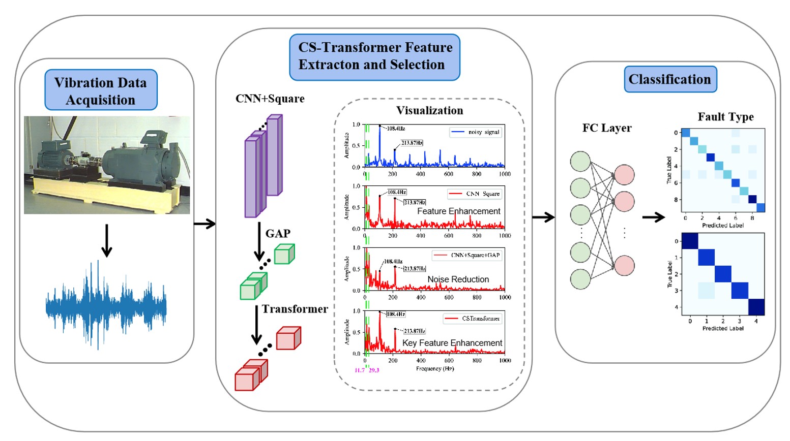
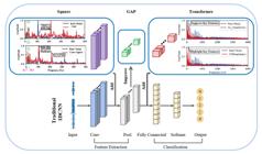
The proposed CS-Transformer framework is illustrated in Figure 1. Based on the traditional one-dimensional convolution neural network (1D CNN), the framework incorporates the following key improvements: Local Feature Enhancement Strategy, Global Feature Aggregation Strategy, and Key Feature Learning Strategy.

Figure 1
Key improvement strategies in the CS-Transformer overall architecture.

2.1 Local Feature Enhancement Strategy (CNN + Square)

While Convolutional Neural Network adaptively learn frequency-domain features of vibration signals (Li et al. 2021; Pang et al. 2024), power spectrum analysis (squared operation) is more commonly used in engineering than amplitude spectrum analysis due to its ability to highlight dominant frequency components and enhance noise resistance. Inspired by this, the proposed approach removes the activation function in conventional 1D CNN and introduces a squared operation to amplify the principal components of features extracted by a single-layer wide convolution, thereby improving feature discriminability in noisy environments.

During the feature extraction process, the convolution operation, through its fixed-sized convolution Layers, captures local features while retaining certain spatial information. Specifically, by sliding the convolution Layers over the input data, the convolution operation can traverse various positions of the data, thereby extracting rich local features (Jiang et al. 2019). In this study, the original 1×$n$ vibration signals will be directly input into the convolution layer. This convolution layer is equipped with $C$ number of wide convolution Layers of length $K$, which can extract features from the data from different perspectives and effectively enhance the spatial modeling ability of the model. To further enhance local features, after the convolution operation, a square operation is introduced to the output results to highlight the principal frequency features of the signal. Compared with traditional activation functions such as ReLU (Rectified Linear Unit) or Softsign, it is more interpretable.

The calculation formula for one-dimensional convolution is:

$y_{ij}={\displaystyle \sum _{k=0}^{K-1}{x}_{i+k}}{\omega }_{jk}+b_j,j=\mathrm{1,2,...,}C$ (1)

If ReLU is used as the activation function, then the output is:

$y_{ij}{}^{\text{relu}}=\max \left(\mathrm{0,}{\displaystyle \sum _{k=0}^{K-1}{x}_{i+k}}.{\omega }_{jk}+b_j\right)$ (2)

If Softsign is used as the activation function, then the output is:

$$y_{ij}^{\text{softsign}}=\frac{{\displaystyle \sum _{k=0}^{K-1}{x}_{i+k}}{\omega }_{jk}+b_j}{1+\left|{\displaystyle \sum _{k=0}^{K-1}{x}_{i+k}}{\omega }_{jk}+b_j\right|}$$ (3)

In this paper, if the result of a one-dimensional convolution is squared, the output is:

$y_{ij}{}^2={\displaystyle \sum _{k=0}^{K-1}{x}_{i+k}^2}{\omega }_{jk}^2+2{\displaystyle \sum _{k=0}^{K-1}{\displaystyle \sum _{m=k+1}^{K-1}{x}_{i+k}{x}_{i+m}}}{\omega }_{jk}{\omega }_{jm}+2b_j{\displaystyle \sum _{k=0}^{K-1}{x}_{i+k}}{\omega }_{jk}+b_j^2$ (4)

Where $x_{i+k}$denotes the value at the k-th position after the i-th position.${\omega }_{jk}$ denotes the weight at the $k$-th position of the $j$-th convolution, $b_j$ represents the corresponding bias term, and $y_{ij}$ corresponds to the output after the squared operation.

Compared with one-dimensional convolution, which performs weighted summation on the signal, squared convolution enhances local features by introducing autocorrelation terms ${\displaystyle \sum _{k=0}^{K-1}{x}_{i+k}^2}{\omega }_{jk}^2$. Meanwhile, cross-correlation terms $2{\displaystyle \sum _{k=0}^{K-1}{\displaystyle \sum _{m=k+1}^{K-1}{x}_{i+k}{x}_{i+m}}}{\omega }_{jk}{\omega }_{jm}$ leverage the cross-association of features at different time points to capture the influence of features at other moments on the current feature, thereby amplifying the target features.

In addition, the primary role of the activation function is to convert the linear weighted sum of a neuron into a nonlinear output, thereby enabling the network to fit more complex and diverse data structures. ReLU and Softsign, as two representative activation functions, correspond to “efficient sparsity” and “smooth boundedness” in nonlinear mapping, respectively. ReLU achieves efficient and sparse feature representation by simply retaining positive values while setting negative values to zero. In contrast, Softsign smoothly compresses inputs into the range (−1, 1), providing bounded features and thus contributing to more stable training. However, the squaring operation strengthens key features through autocorrelation and cross-correlation terms. This approach not only avoids the feature loss seen in ReLU due to zeroing negative values, but also differs from compression of Softsign by amplifying the differences between features, thereby highlighting important features more efficiently.

2.2. Global Feature Aggregation Strategy (GAP)

Pooling operations reduce feature dimensionality through pooling layers while preserving critical information and suppressing local noise (Huang et al. 2019; Li et al. 2022). This study further introduces global average pooling to diminish the reliance of the model on local details and boost the robustness of global features against noise interference.

Global average pooling is implemented for the features extracted by convolution, which strengthens the model's attention on broader feature patterns. This helps improve the model's generalization capability and ensures its computational efficiency. The output feature dimension of the convolution is $y\in R^{T\text{×}C}$, where $T$ represents the sequence length and $C$ is the number of convolution kernels. The global average pooling process is as follows:

$z_j=\frac{1}{T}{\displaystyle \sum _{i=1}^T{y}_{ij}},j=\mathrm{1,2,...,}C$ (5)

Where $z_j$ represents the global average value output by the $j$-th convolution kernel, and the dimension of the final global feature vector $z$ is $R^C$.

2.3. Key Feature Learning Strategy (Single-layer Transformer Encoder)

The self-attention mechanism in Transformer captures long-range dependencies and focuses on key features through dynamic weight allocation (Vaswani et al. 2017). This implies that in high-noise scenarios, the self-attention mechanism can amplify target signals via global contextual information, addressing the vulnerability of Convolutional Neural Networks (CNN) to noise arising from their reliance on local features (Fang et al. 2022). Building on the two aforementioned optimization strategies, this study leverages the self-attention mechanism in the Transformer encoder to integrate global contextual information, enabling efficient fault diagnosis in strong noise environments. As shown in Figure 2, the Transformer encoder architecture is composed of: (a) Multi-Head Attention Mechanism, (b) Residual Connections, (c) Feed-Forward Neural Network (FFN), and (d) Normalization.

Figure 2
Structure diagram of the Transformer encoder layer, (a) Multi-Head Attention Mechanism, (b) Residual Connection, (c) FFN, (d) Normalization.

The self-attention mechanism of the Transformer encoder can conduct deep interaction and fusion among global feature vectors. It can mine the correlations hidden in global features by adaptively learning the weight relationships among different features. The input vector is $z=\left[z_1,z_2\mathrm{,...,}{z}_C\right]\in R^C$. Firstly, it is transformed through a linear transformation to generate Query ($Q$), Key ($K$) and Value ($V$):

$$\left\{\begin{array}{c}Q=z{W}_Q\\ K=z{W}_K\\ V=z{W}_V\end{array}\right.,\begin{array}{cc}& W_Q,W_K,W_V\in R^{C\times d_k}\end{array}$$ (6)

Here, $d_k$ represents the attention dimension, and $W_Q,W_K,W_V$ denotes the learnable parameters.

Calculate the attention weights:

$A=\mathrm{softmax}\left(\frac{Q{K}^T}{\sqrt{d_k}}\right)$ (7)

The attention output is:

$z^{\text{'}}=AV$ (8)

Where $A\in R^{C\times C}$ represents the attention weight matrix, and $z^{\text{'}}\in R^{C\times d_k}$is the updated global feature.

3 EXPERIMENTAL VERIFICATION AND RESULT ANALYSIS

In this section, two types of experiments will be conducted to validate the effectiveness and generalization capacity of the proposed model. Firstly, an ablation experiment will be conducted by gradually removing or replacing the key components in the model to evaluate the contribution of each part to the overall performance, thereby revealing the rationality of the model design and the effectiveness of the feature extraction ability. Secondly, a performance comparison experiment will be carried out to compare the performance with various advanced models that are currently available, especially in terms of accuracy, robustness, and classification efficiency under different noise environments, in order to comprehensively illustrate the benefits of the proposed model for bearing fault diagnosis.

The experiments will be conducted on a Windows 10 operating system and implemented in Python 3.8 using the PyTorch framework. Hardware acceleration was provided by an NVIDIA RTX 3060 GPU with CUDA 11.3, supporting both model training and inference. All experiments were conducted in strict accordance with the principle of independent replication. Each experimental setup was repeated five times, and the average results were computed to effectively control random errors and ensure the reproducibility and reliability of the findings.

3.1. Experimental Preparation

3.1.1. Experimental Dataset

The experiments employ bearing datasets from Case Western Reserve University (CWRU) and Paderborn University, which collectively encompass diverse fault types and damage severity levels. These datasets offer comprehensive data foundations for analyzing vibration signatures under varying operational conditions.

(1) Case Western Reserve University (CWRU) Bearing Dataset

The data employed for the experiments in this study came from the publicly available Case Western Reserve University (CWRU) Bearing Data Center dataset. The research focuses on faulty bearings operating under 0 horsepower load with defect diameters of 0.1778mm, 0.3556mm, and 0.5334mm, a rotational speed of 1797r/min, and a sampling frequency of 12kHz. The selected fault locations include Ball Fault, Inner Race Fault, and Outer Race Fault at the 6 o'clock direction. Figure 3 illustrates time-domain and frequency-domain plots of randomly sampled signals under four operational states. Specific bearing conditions, fault diameters, and class labels are detailed in Table 1.

Figure 3
Sample signals from the CWRU dataset used in experiments, (a) Normal, (b) Inner, (c) Ball, (d) Outer .

Table 1
Bearing States and Label Settings for the CWRU Dataset

Bearing Condition	Fault Diameter (mm)	Label
Normal	—	0
Inner Race Fault	0.18	1
Ball Fault	0.18	2
Outer Race Fault	0.18	3
Inner Race Fault	0.36	4
Ball Fault	0.36	5
Outer Race Fault	0.36	6
Inner Race Fault	0.54	7
Ball Fault	0.54	8
Outer Race Fault	0. 54	9

For each fault condition, the experimental bearings generate 102,400 data points. These are segmented into 4,096 data points per segment using a sliding window approach with a 50% overlap ratio, yielding 50 samples per class. The dataset is then divided into 70% training, 10% validation, and 20% testing subsets through random stratified sampling.

(2) Paderborn University Bearing Dataset

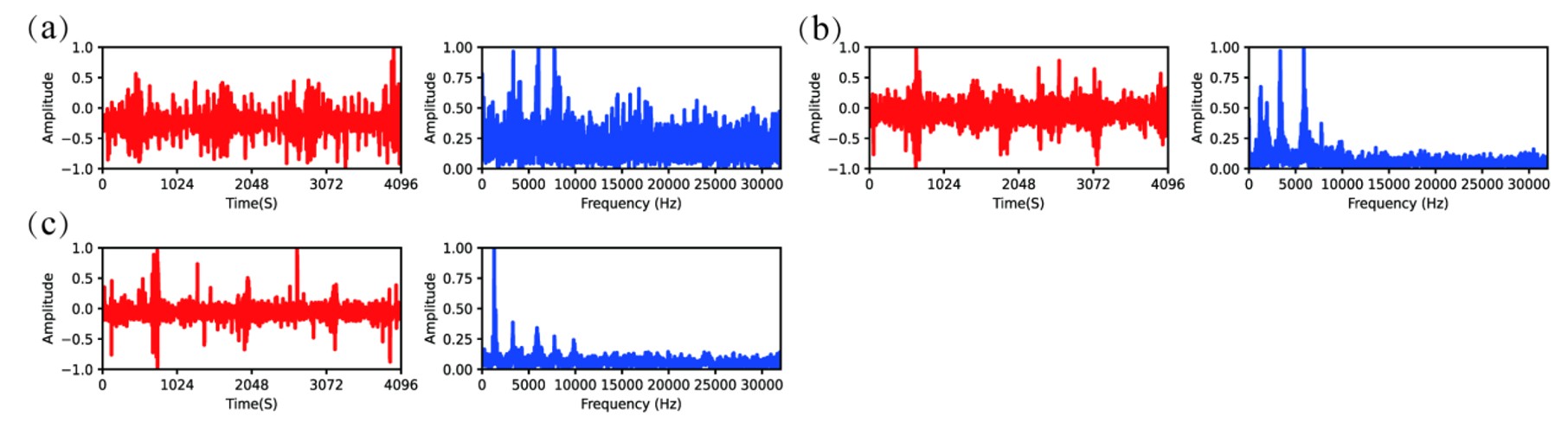
This dataset from Paderborn University in 2016 was provided by Lessmeier et al. (2016). The data sources are categorized into two experimental types: artificially induced damage and real-world operational damage, each containing three bearing states: healthy, inner race fault, and outer race fault. Figure 4 presents time-domain and frequency-domain plots of randomly sampled signals under these three states.

Figure 4
Sample signals from the Paderborn dataset used in experiments(a) Normal (b) Outer (c) Inner.

The study focuses on the vibration signals of bearings under artificial damage conditions, under a 0.7 Nm load torque (M) and bearing radial force (F) of 1000 N, and a rotational speed of 1,500 r/min. The severity of the damage is classified into two levels: level 1 represents minor damage, while level 2 indicates the most severe damage. The sampling frequency is 64 kHz. Specific bearing states, damage levels, and class labels are listed in Table 2. For each fault category, 50 samples are extracted, each consisting of 4096 data points. Sample quantities are augmented using a sliding window approach with a 50% overlap ratio. The dataset is partitioned into 70% training, 10% validation, and 20% testing subsets following stratified random sampling.

Table 2
Bearing Conditions and Label Settings for the Paderborn Dataset

Bearing Condition	Damage Severity	Label
Normal/K001	—	0
Outer Race Fault/KA07	1	1
Inner Race Fault/Ki05	1	2
Outer Race Fault/KA08	2	3
Inner Race Fault/Ki07	2	4

3.1.2. Network Structure Optimization and Parameter Setting

This section will discuss how to select an appropriate network architecture to meet the specific requirements of a task, as well as how to effectively configure model parameters to enhance training effectiveness and generalization performance of the model.

(1) Network Structure Optimization

This experiment focuses on the parameter optimization of the diagnostic model. Based on the CWRU dataset, it deeply explores the impact of different parameter settings on the model's accuracy, aiming to find the optimal parameter combination of the model under noise-free and strong noise (-6db) conditions.

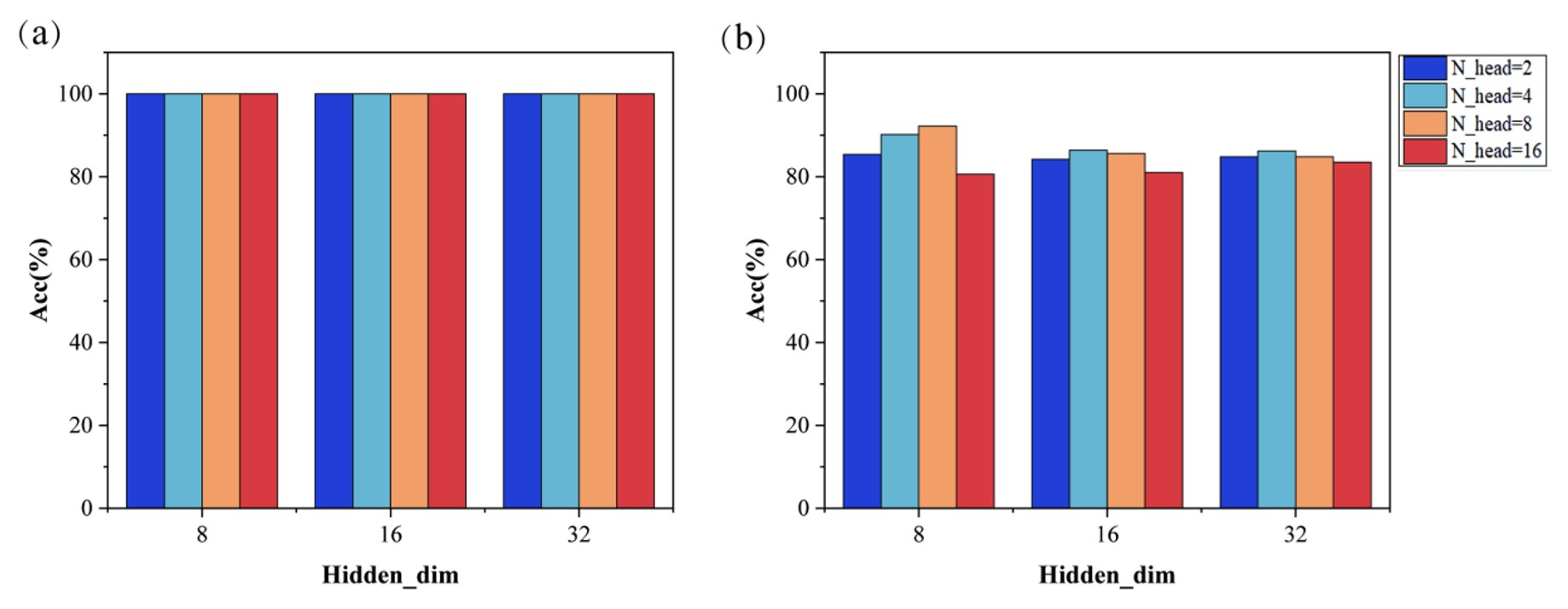
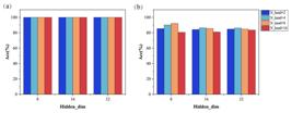
Figure 5 shows the classification accuracy of the model based on the CWRU dataset under the same convolution Layer size (256) and encoder layer number, with different hidden layer dimensions (Hidden_dim = 8, 16, 32) and different numbers of attention heads (N_head = 2, 4, 8, 16).

Figure 5
Experimental diagram of parameter optimization under different conditions based on the CWRU dataset (a) Original signal, (b) Noisy signal.

Figure (a) shows the results in the noise-free environment, as the dimension of the hidden layer increases, the classification accuracy remains at a relatively high level and is almost unaffected by the number of attention heads. This indicates that under the noise-free condition, the model has a relatively small dependence on different attentions and hidden layer dimensions.

Figure (b) reflects the influence of model structure parameters on accuracy in the presence of noise. When the dimension of the hidden layer is small (Hidden_dim = 8), the accuracy increases significantly with the increase in the number of attention heads. However, when the dimension of the hidden layer increases to 16 and 32, this improvement trend tends to flatten out or even decrease.

The optimal parameters of the model network structure at this time are: Kernel_size = 256, Transformer_Encoder_Layer = 1, Hidden_dim = 2, N_head = 8.

(2) Network structure parameter setting

The configuration parameters setting of the bearing fault diagnosis model proposed in this paper is shown in Table 3.

Table 3
Model configuration details

Number of Network Layers	Structure Name	Detailed Parameters
		Input	Kernel size	Layer number	Act	Hidden_dim	N_head	Output
0	Input Layer	1×4096	/	/	/	/	/	1×4096
1	Convolution Layer	1×4096	256	16	/	/	/	16×3843
2	Square Layer	16×3843	/	/	/	/	/	16×3843
3	GAP Layer	16×3843	/	/	/	/	/	16×1
4	Encoder Layer	1×16	/	/	/	8	8	1×16
5	FC Layer	1×16	/	/	/	/	/	16×10

The training parameters for the diagnostic model are presented in Table 4. The Adam optimizer was employed for training the model, with cross-entropy serving as the loss function. Experimental settings included batch size of 32, training epochs of 120, learning rate of 0.007, weight decay of 1e-3, and dropout of 0.3.

Table 4
Model Training Parameters

Optimizer	Loss function	Batch-size	Number of epochs	Learning Rate	Weight-decay	Dropout
Adam	Cross entropy	32	120	0.007	1e-3	0.3

(3) Signal Sampling Length

Vibration signals contain abundant fault-related characteristics. Selecting an appropriate signal sampling length is crucial for ensuring that samples accurately reflect the original signal. In essence, the sampling length is determined by the minimum time needed to obtain the lowest - frequency component in the signal for analysis.

In rolling bearings, the cage fault frequency usually represents the lowest fault frequency (e.g., 11.93 Hz in CWRU datasets). For CWRU cage faults, the calculated signal length is approximately 1006 samples (12,000 ÷ 11.93 ≈ 1006), and multiplying by 4 gives 4024 (with 12 kHz as the sampling frequency). To guarantee complete data cycles and eliminate edge effects, the experimental data length is set to 4096. This setting ensures that signal samples include over two full cage fault cycles.

3.2. Experiment on the Effectiveness of Improved Strategies

To prove the validity of the improved strategies, controlled variable experiments were conducted based on the CWRU bearing dataset.

3.2.1. Single Strategy Effectiveness Verification Experiment

(1) Validation Experiment on the Effectiveness of Local Feature Enhancement Strategy

In order to precisely extract the principal features of the signal, the proposed strategy introduces a squaring operation after the traditional convolution layer. Through visualization analysis of the output features of the convolution, this approach is compared with conventional nonlinear activation functions (e.g., ReLU or Softsign) to verify the advantages of the squaring operation in enhancing local feature representation and highlighting critical frequency information.

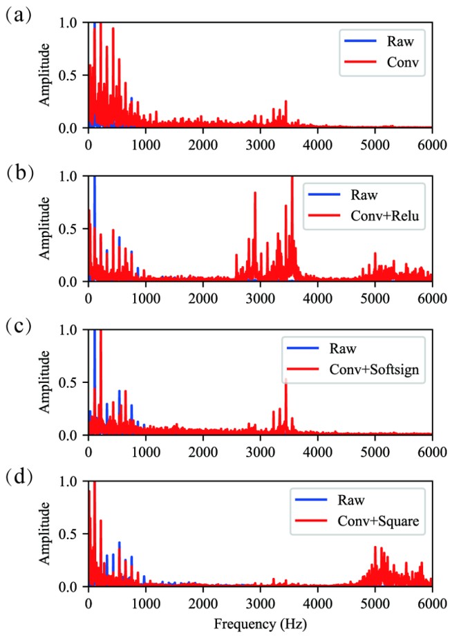
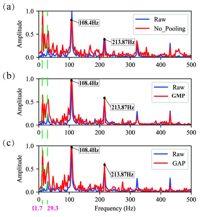
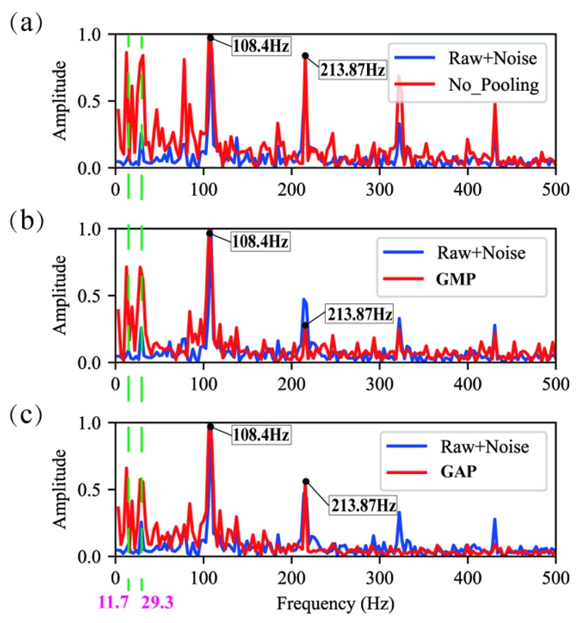
Experimental results indicate that this strategy effectively highlights the primary frequency components of the signal, while also enhancing the interpretability of the model. Figures 6 and 7 illustrate the envelope spectra of signals extracted by convolutional layers with different activation functions (including ReLU, Softsign, and Square) under both original and noisy signals (red lines). The envelope spectra of the original signal and noisy signal are represented by the blue line. Among these, 108.4 Hz represents the outer race fault characteristic frequency, 213.87 Hz is its second harmonic, and other low frequencies (such as 11.7 Hz and 29.3 Hz, corresponding to cage fault and harmonics, respectively) are marked with green dashed lines. The first convolutional layer includes either convolution and squaring operation or convolution and activation function in this section.

Figure 6
Envelope spectra of convolution layer output signals under different activation functions (original signals)

Figure 7
Envelope spectra of convolution layer output signals under different activation functions (noisy signals)

It can be observed that, compared to other activation functions, the square operation demonstrates a stronger ability to highlight low frequencies (11.7 Hz and 29.3 Hz) and the fault characteristic frequency (108.4 Hz), while minimizing the risk of feature frequency confusion and effectively suppressing noise. This result indicates that the local feature extraction strategy, which performs receptive field sliding sampling through convolutional kernels and combines the square operation to optimize outer race fault characteristic frequencies, significantly enhances feature extraction capability.

Figures 8 and 9 respectively present the full signal envelope diagrams extracted by convolution layers utilizing different activation functions (including ReLU, Softsign, and Square) under original signals and noisy signals.

Figure 8
The full envelope spectrum of convolution layer output signals under different activation functions (original signals).

Figure 9
The full envelope spectrum of convolution layer output signals under different activation functions (noisy signals).

It can be observed that regardless of the original or noisy signals, convolution layers with different activation strategies all learned non-fault high-frequency features, whereas bearing defects typically induce low-frequency impact excitations. In contrast, the squaring operation in noisy signals significantly suppresses background noise and non-fault high-frequency features, clearly characterizing the outer race fault characteristic frequency and demonstrating strong target feature extraction capabilities.

(2) Validation Experiment on the Effectiveness of Global Feature Aggregation Strategy

For vibration-based diagnostics, signal features often exhibit prominent global characteristics. Effective capture of these global patterns is critical for improving diagnostic accuracy. However, directly extracting raw or local features may lead to the loss of critical global information while increasing sensitivity to noise. To address this challenge, a global feature aggregation strategy was designed. This approach integrates global responses of the signal through pooling operations, enhancing key features while mitigating noise interference.

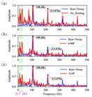
Figures 10 and 11 respectively present the envelope spectra extracted by the first convolutional layer of each strategy (red), under both original and noisy signal conditions. The first convolutional layer includes convolution and squaring operation in this section.

Figure 10
The learned envelope spectra of the first convolution layer under different pooling strategies (original signals).

Figure 11
The learned envelope spectra of the first convolution layer under different pooling strategies (noisy signals).

No Pooling: For the original signal, the fault characteristic frequency 108.4 Hz is not significantly prominent compared to other frequencies, resulting in a relatively flat response. This can lead to insufficient emphasis on key fault frequencies in diagnostic tasks and a lack of feature saliency. For noisy signals, the amplitude of 108.4 Hz in the spectrum is too close to its second harmonic (213.87 Hz) and low frequencies (11.7 Hz and 29.3 Hz), which can easily cause feature confusion.

Global Max Pooling (GMP): It effectively extracts the most prominent fault characteristic frequency (108.4 Hz) from the spectrum. Whether for original and noisy signals, the key fault frequency components are significantly enhanced after applying global max pooling; however, the noise suppression effect remains insufficient.

Global Average Pooling (GAP): For the original signals, the fault characteristic frequency at 108.4 Hz is prominently highlighted, while its harmonic at 213.87 Hz is also clearly represented, and other non-characteristic frequencies are effectively suppressed. For noise-added signals, GAP enhances the features while avoiding noise amplification, resulting in overall features that are smoother and more orderly. Compared to the original signal, the envelope spectrum processed by GAP is noticeably smoother, demonstrating a stronger capability to suppress background noise.

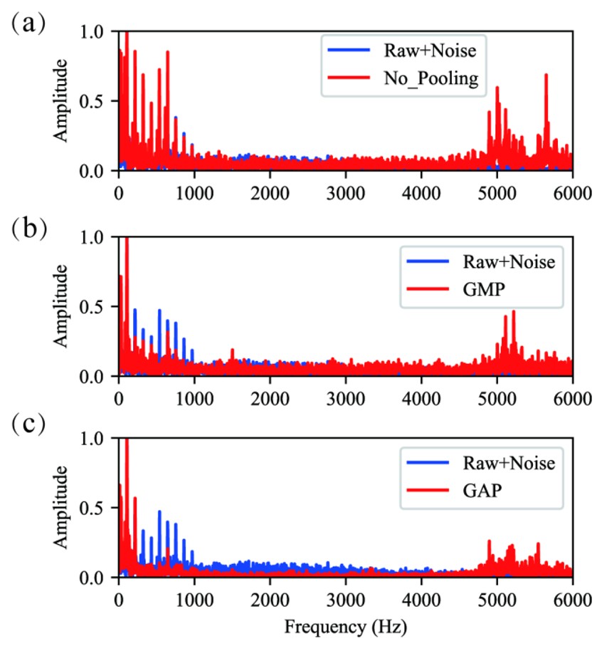
Figures 12 and 13 respectively present the complete envelope diagrams of the signals extracted from the first convolution layer using different pooling strategies, under both original and noisy signal conditions.

Figure 12
The complete envelope spectra learned by the first convolution layer under different pooling strategies (original signals).

Figure 13
The complete envelope spectra learned by the first convolution layer under different pooling strategies (noisy signals).

The figures reveal that convolution layers with different pooling strategies all learn non-fault high-frequency features, yet global average pooling significantly suppresses both non-fault high-frequency features and background noise in noisy signals, making it easier to capture critical characteristic frequencies.

(3) Validation Experiment on the Effectiveness of Key Feature Learning Strategy

This strategy employs the multi-head attention mechanism of the Transformer encoder to deeply interact and fuse global features extracted by diverse convolution kernels. It adaptively learns the weight relationships between features pooled from 16 convolution kernels, enhancing the model's global feature representation capability. By effectively mining latent feature correlations, it achieves precise extraction of critical fault-related features.

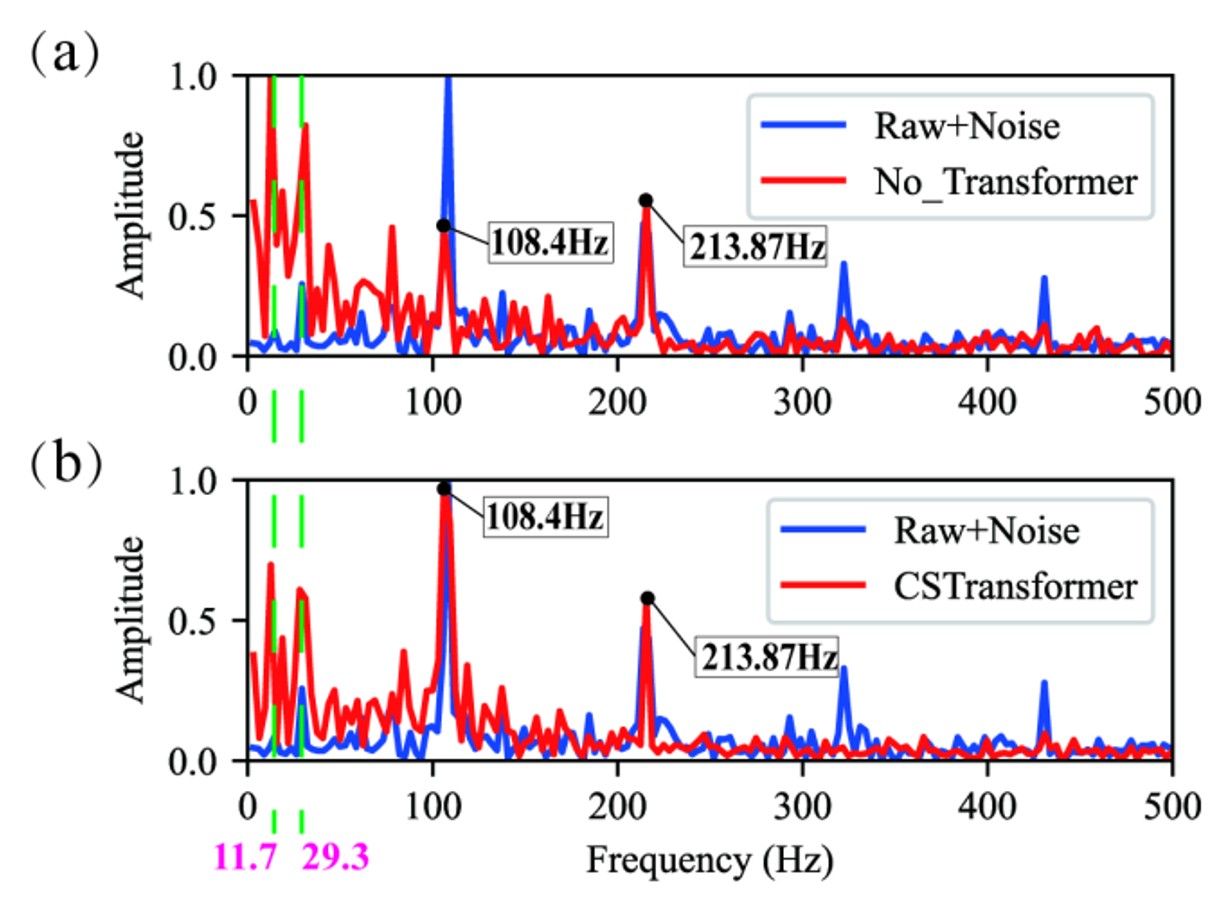
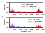
Figures 14 and 15 illustrate the changes in the learned envelope spectra of first convolution layer after integrating the Transformer encoder layer. The first convolutional layer includes convolution and squaring operation in this section.

Figure 14
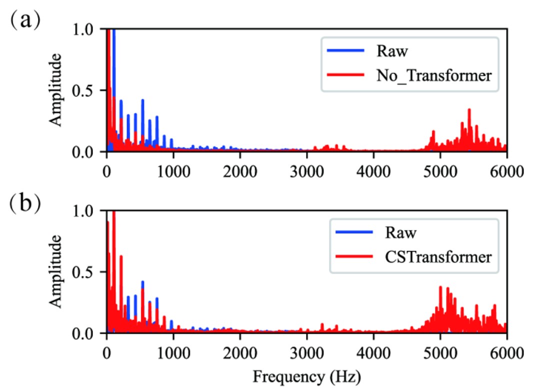
Comparison of the envelope spectra of signals learned by the first convolution layer before and after integrating Transformer (original signals).

Figure 15
Comparison of the envelope spectra of signals learned by the first convolution layer before and after integrating Transformer (noisy signals).

For the original signals, after removing the Transformer encoder layer from the model in subfigure (a), its ability to capture the fault frequency of 108.4 Hz is relatively weak, and the amplitude captured is significantly lower than that of the original signal. In subfigure (b), compared with the original signal (blue line), CS-Transformer (red line) at 108.4 Hz is more prominent in terms of feature frequency. In the presence of noise, after removing the Transformer encoder layer from the model in subfigure (a), CS-Transformer's ability to capture 108.4 Hz significantly decreases, and it is also significantly weaker compared to the original noisy signal. This indicates that the model without Transformer has weakened feature extraction ability in the presence of noise. In subfigure (b), CS-Transformer has a significantly stronger learning effect on 108.4 Hz, and the amplitude is similar to or even enhanced compared to the original noisy signal. The non-feature frequencies are suppressed, and the fault frequency is more prominent.

Figures 16 and 17 respectively present the complete envelope spectra of signals extracted by the first convolution layer before and after integrating Transformer encoder layers into the model, under both original and noisy signal conditions.

Figure 16
Comparison of the envelope spectra of signals learned by the first convolution layer before and after integrating Transformer (original signals).

Figure 17
Comparison of the envelope spectra of signals learned by the first convolution layer before and after integrating Transformer (noisy signals).

As shown in the figures, both before and after integrating the Transformer encoder layer, the convolution layer learned non-fault-related high-frequency features. However, under noisy signal conditions, CS-Transformer demonstrates superior performance in suppressing these non-fault-related high-frequency features and background noise, thereby more prominently highlighting the critical characteristic frequencies.

In conclusion, the Transformer encoder layer significantly enhances the model's ability to extract fault features, especially in the presence of noise, it shows stronger anti-noise performance.

3.2.2. Experiment on the Effectiveness of Combined Strategies.

This section validates the effectiveness and interpretability of CS-Transformer from two perspectives: the impact on classification performance and feature extraction mechanisms.

(1) Effectiveness Analysis Based on Classification Results

A comparison of the feature extraction performance of different combined strategies is conducted. The proposed strategies include: Local Feature Enhancement Strategy (A: CNN+Square), Global Feature Aggregation Strategy (B: GAP), and Key Feature Learning Strategy (C: Transformer Encoder Layer).

The proposed combination (A + B + C) exhibits significant advantages in diagnostic performance under low signal - to - noise ratio conditions (SNR = -6). Its comprehensive metrics far exceed those of other combinations, as shown in Table 5.

Table 5
Diagnostic Accuracy of Models under Different Combinations (SNR = -6)

Combination Strategy	Accuracy(%)	Precision(%)	Recall(%)	F1-score(%)	Parameters	Time (s)
A	30.0	37.0	30.0	30.0	4112	9
C	36.0	37.0	40.0	35.0	5746	292
A+B	89.2	89.2	89.2	89.2	4282	9
A+C	25.4	22.8	25.8	23.4	5714	266
A+C+B	49.2	46.4	51.0	48.0	5714	266
A+B+C	91.6	92.6	91.6	91.6	5714	16

First, in terms of diagnostic performance, the combination A + B + C achieves an accuracy of 91.6%, significantly outperforming all comparative methods. The performance of using A or C alone is relatively low. While the A + B combination shows a notable improvement (with an accuracy of 89.2%), it still falls short of the final performance of A + B + C. This indicates that the inclusion of module C further enhances the feature extraction capability, achieving a higher diagnostic accuracy through collaborative optimization of multiple modules.

Secondly, regarding parameter count and running time, the A + B + C combination strikes a balance between performance and computational efficiency. Although its parameter count is slightly higher than the A and A + B combinations (4112 and 4828, respectively), it reduces the redundant parameters compared to the less effective combinations A + C + B and the single module C, contributing to model lightweighting. Additionally, its running time is 16 seconds, considerably lower than that of the single module C and other more complex combinations, indicating that A + B + C not only improves diagnostic accuracy but also enhances computational efficiency.

(2) Clustering Effectiveness Analysis Based on t-SNE

Figure 18 makes use of t-SNE to transform high-dimensional data into a low-dimensional representation, while preserving the relative positional relationships between data points as much as possible. This systematically evaluates the clustering performance of each combined model.

Figure 18
The t-SNE clustering results of each combined model, (a) A, (b) C, (c) A+B, (d) A+C, (e) A+C+B, and (f) A+B+C.

It can be observed that the clustering distribution of data points varies significantly across the different subfigure. In subfigure (f), data points of the same class are relatively clustered, forming a distinct cluster, which indicates that the CS-Transformer demonstrates better clustering performance on these data compared to other models. Therefore, the combination of Local Feature Enhancement Strategy (A), Global Feature Aggregation Strategy (B), and Key Feature Learning Strategy (C) in A + B + C results in a significant enhancement of the model's diagnostic capabilities.

(3) Effectiveness Analysis Based on Feature Extraction Mechanism

By investigating the envelope spectra of the output signals from the first convolution layer under different combination strategies, the effectiveness of CS-Transformer in feature extraction is analyzed.

Figures 19 and 20 show the comparisons of envelope spectra of first convolution layer extracted by each combination strategy for inner ring and outer ring fault samples, respectively, under the same noise conditions. The envelope spectra of the original signal are represented by the blue line. Here, 162.19 Hz is the inner race fault frequency; 108.4 Hz is the outer race fault frequency; and 213.87 Hz is its second harmonic. Other low frequencies, marked by green dashed lines (11.7 Hz and 29.3 Hz), correspond to cage fault and their harmonics. The first convolutional layer includes convolution and squaring operation in this section.

Figure 19
Learned envelope spectra of the first convolution layer for different combinations on noisy signals (inner).

Figure 20
Learned envelope spectra of the first convolution layer for different combinations on noisy signals (outer).

As shown in Figure 19, Combination A does not produce a significant peak at the characteristic frequency of 162.19 Hz, resulting in an overall relatively flat response. Combination A+B, while suppressing some noise, shows overly dense and closely-spaced low-frequency features in the 0-200 Hz range, which can lead to feature confusion. Combination A+C exhibits a relatively flat response and shows poor suppression of non-characteristic frequencies, failing to highlight the 162.19 Hz frequency. Combination A+C+B improves the extraction of the characteristic frequency but still exhibits noticeable fluctuations at non-characteristic frequencies. In comparison to the above strategies, Combination A+B+C (subfigure (e)) performs the best, producing a relatively prominent peak at the characteristic frequency of 162.19 Hz. Meanwhile, interference and background noise in the non-characteristic frequency regions are significantly suppressed, reducing the likelihood of feature confusion and demonstrating strong feature extraction and noise suppression capabilities.

From Figure 20, Combination A fails to sufficiently enhance the characteristic frequency of 108.4 Hz, resulting in a relatively flat performance. Combination A+B achieves some noise suppression, but the amplitude of the characteristic frequency is significantly lower than that of the original signal. Combination A+C also shows a relatively flat response; although it enhances the characteristic frequency of 108.4 Hz and its second harmonic, the amplitudes of the two frequencies are too close, making it difficult to highlight the characteristic frequency and thus affecting fault diagnosis accuracy. Combination A+C+B demonstrates a feature extraction capability similar to that of Combination A+C, which may lead to misidentification of fault features. Compared with the above strategies, Combination A+B+C (subfigure (e)) still performs the best, achieving significantly superior extraction of the characteristic frequency and suppression of non-characteristic frequencies, which facilitates more accurate fault classification.

In summary, Combination A + B + C achieves precise extraction of characteristic frequencies and effective suppression of background noise, resulting in the best feature extraction performance and overall outstanding capabilities.

3.3. Comparative Experiment on Model Diagnostic Performance

For assessing the efficacy of various models in diagnosing bearing failures, a testing framework with noisy fault data was designed to comprehensively evaluate the models' robustness against noise. Gaussian white noise at five different levels (10 dB, 4 dB, 0 dB, -4 dB, and -6 dB for the signal-to-noise ratio) was incorporated into the dataset. Under the same experimental conditions, 1D CNN (Chen et al. 2020), ELCNN (Pang et al. 2024), CNNLSTM (Khorram et al. 2021), and WDCNN (Zhang et al. 2017) were selected as comparative models for testing.

3.3.1. Comparison Experiment Based on the CWRU Dataset

This experiment conducts performance comparison tests of models using the CWRU dataset.

(1) Evaluation of Different Models' Classification Accuracy Under Noise-Free Conditions

In this experiment, the CS-Transformer is compared with other models under noise-free conditions using the CWRU dataset to validate the classification performance. The classification results are shown in Table 6.

Table 6
Comparison of classification performance of different models for the original signals

	1D CNN	ELCNN	WDCNN	CNNLSTM	CS-Transformer
ACC (%)	84.8	99.0	85.0	100.0	100.0
Pre (%)	84.0	99.0	85.0	100.0	100.0
Recall (%)	85.2	99.0	84.6	100.0	100.0
F1 (%)	84.8	99.0	84.8	100.0	100.0
Time (s)	24	7	20	43	16

For the original signals, the experimental outcomes from the CWRU dataset suggest that both ELCNN and CNNLSTM models perform well across various classification metrics, although their classification performance and computational efficiency are slightly inferior to that of the CS-Transformer. In contrast, the classification performance of both 1D CNN and WDCNN is relatively poor. In conclusion, the CS-Transformer achieves 100% in all classification metrics while maintaining superior operational efficiency.

(2) Evaluation of Different Models' Classification Accuracy Under Different SNR

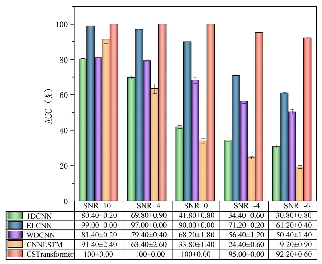
This experiment compares the classification accuracy of the CS-Transformer with other models across various signal-to-noise ratio (SNR) levels using samples from the CWRU dataset. Figure 21 visually illustrates the noise resistance performance of different models in various noise environments.

Figure 21
Performance Comparison of Different Models Under Varying Signal-to-Noise Ratios.

From Figure 21, the CS-Transformer maintains high accuracy consistently, significantly exceeding that of other models in the low SNR range (e.g., -6 dB to 0 dB). As the SNR rises, the CS-Transformer maintains a high level of accuracy.

(3) Comparison of Confusion Matrices for Diagnostic Results of Different Models at the Same SNR

Figure 22 displays diagnostic outcomes via confusion matrices, comparing models at at an equal signal - to - noise ratio (SNR=-6).

Figure 22
Classification confusion matrices under the same SNR for different models, (a) 1DCNN, (b) ELCNN, (c) WDCNN, (d) CNNLSTM, (e) CS-Transformer.

It can be seen from the figures that the CS-Transformer model exhibits stronger classification performance under high noise conditions, accurately identifying multiple fault types. In contrast, other models demonstrate poorer classification performance in low signal-to-noise ratio environments, particularly showing significant confusion for certain categories, with CNNLSTM performing the worst.

(4) Visualization of convolution Output Envelope Spectrum for Different Models at the SNR

Figures 23 and 24 illustrate the comparison between the envelope spectra extracted by the first convolution layer of each model under both original and noisy signals, respectively. The envelope spectra of the original signal are represented by the blue line. The outer race fault's characteristic frequency is denoted by 108.4 Hz, and 213.87 Hz represents its second harmonic. The first convolutional layer of the CS-Transformer includes convolution and squaring operation, while the first convolutional layer of the contrast model includes convolution and the corresponding activation function in this section.

Figure 23
Learned envelope spectra of the first convolution layer across different models (original signals).

Figure 24
Learned envelope spectra of the first convolution layer across different models (noisy signals).

For the original signals, the 1DCNN、 ELCNN、 CNNLSTM can enhance 108.4 Hz, but its ability to capture the second harmonic feature is constrained. WDCNN does not effectively highlight the 108.4 Hz frequency, captures high-frequency non-characteristic frequencies. In contrast, the CS-Transformer excels in highlighting both the characteristic frequency and the harmonic while effectively enhancing low-frequency features (11.7 Hz and 29.3 Hz).

In a noisy environment, noise robustness becomes critical. Both 1DCNN and ELCNN demonstrate poor performance in extracting low-frequency features (11.7 Hz and 29.3 Hz). WDCNN does not effectively highlight the 108.4 Hz frequency, while CNNLSTM, although capable of enhancing the 108.4 Hz frequency, suppresses the 213.87 Hz frequency and has limited capacity for extracting low-frequency features. In contrast, CS-Transformer exhibits superior performance, accurately enhancing features at the fault characteristic frequency, its harmonic, and low frequencies, while significantly mitigating the effects of noise.

By visualizing the frequency domain features extracted by the convolution of different models at the same SNR, it is patently clear that the CS - Transformer exhibits superior noise resilience, with accuracy markedly higher than that of other models. This confirms its superiority and interpretability in fault diagnosis tasks. Furthermore, the CS-Transformer outperforms the original signal in extracting features from noisy signals, showcasing enhanced robustness and reliability.

3.3.2. Performance Comparison Experiments Based on the Paderborn Dataset

To validate the generalization of the models, further experiments were conducted on the Paderborn dataset.

(1) Evaluation of Different Models' Classification Accuracy Under Noise-Free Conditions

This experiment compares the CS-Transformer with other models based on the Paderborn dataset in a noise-free environment to assess the generalization of the models. The classification results are shown in Table 7.

Table 7
Comparison of classification performance of different models for the original signals(Paderborn dataset)

	1D CNN	ELCNN	WDCNN	CNNLSTM	CS-Transformer
ACC (%)	88.8	92.0	92.0	44.0	100.0
Pre (%)	90.2	92.0	92.4	42.0	100.0
Recall (%)	88.8	92.0	91.0	44.0	100.0
F1 (%)	88.2	92.0	92.2	42.0	100.0
Time (s)	16	7	20	37	16

For the original signals, experimental results based on the Paderborn dataset indicate that the classification metrics of the ELCNN and WDCNN models slightly lag behind those of the CS-Transformer across various categories. The 1DCNN demonstrates the next-best classification capability, while the CNNLSTM exhibits the poorest classification performance. In contrast, the CS-Transformer still achieves 100% across all classification metrics, maintaining high operational efficiency.

(2) Evaluation of Different Models' Classification Accuracy Under Different SNR

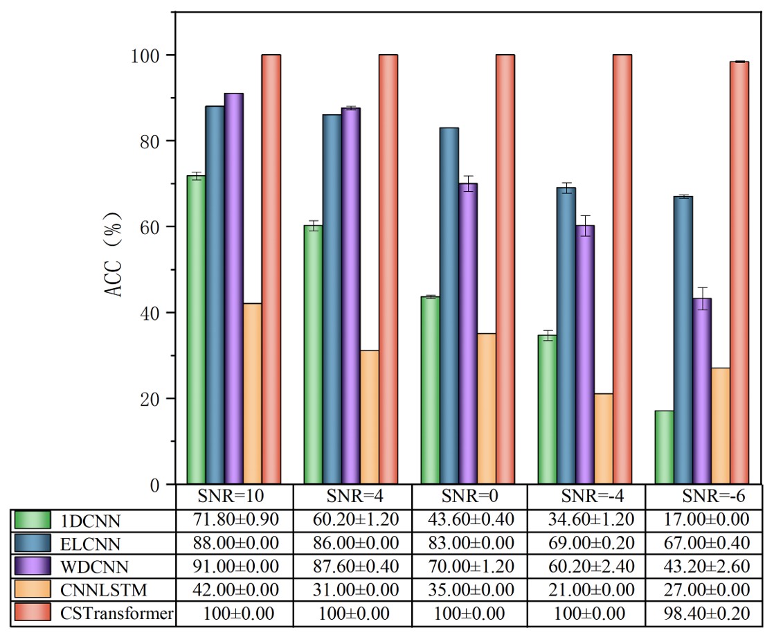
This experiment compares the classification accuracy of the CS-Transformer with other models on samples from the Paderborn dataset under varying signal-to-noise ratios, as illustrated in Figure 25.

Figure 25
Performance Comparison of Various Models Under Varying Signal-to-Noise Ratios.

As illustrated in the figure, the classification accuracy of all models improves with increasing SNR, but performance disparities are pronounced. CS-Transformer demonstrates consistently superior classification performance across all SNR levels, maintaining stability even in low SNR environments. Notably, its accuracy significantly surpasses other models under low SNR conditions, underscoring its exceptional noise robustness.

(3) Comparison of Confusion Matrices of Diagnostic Results for Various Models at the identical SNR

Figure 26 displays diagnostic outcomes via confusion matrices, comparing models at consistent SNR.

Figure 26
Classification confusion matrices of different models, (a) 1D CNN, (b) ELCNN, (c) WDCNN, (d) CNNLSTM, (e) CS-Transformer.

Based on the confusion matrix, the CS-Transformer excels at classification within the Paderborn dataset. The ELCNN exhibits suboptimal but relatively good classification performance, correctly classifying most categories while still showing slight misclassifications in some categories. The CNNLSTM and WDCNN models demonstrate more pronounced misclassification issues. The 1DCNN performs the worst, struggling to effectively accomplish the fault classification task.

(4) Visualization of Convolution Layer Output Envelope Spectra of Different Models at the same SNR

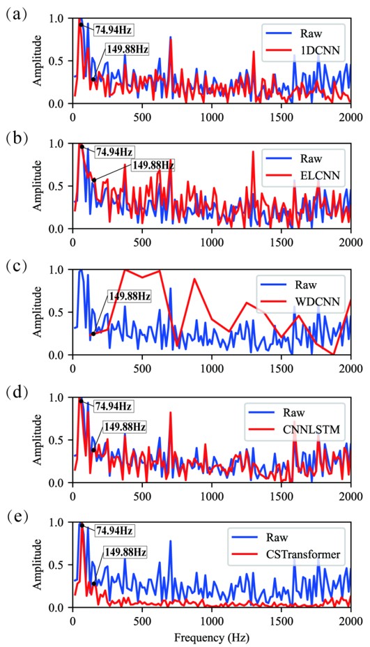
Figures 27 and 28 illustrate the comparison between the envelope spectra extracted by the first convolution layer of each model, under both original and noisy signals, respectively. The envelope spectra of the original signal are represented by the blue line. Here,the outer race fault's characteristic frequency is denoted by 74.94 Hz, while 149.88 Hz corresponds to its second harmonic frequency. The first convolutional layer of the CS-Transformer includes convolution and squaring operation, while the first convolutional layer of the contrast model includes convolution and the corresponding activation function in this section.

Figure 27
Envelope spectra learned by the first convolution layer across different models (Original signal).

Figure 28
Envelope spectra learned by the first convolution layer across different models (Noisy signal).

From the figures, it can be observed that 1DCNN, ELCNN, WDCNN, and CNNLSTM amplify non-characteristic frequencies without significantly highlighting the characteristic frequency of 74.94 Hz. This indicates a limited ability to extract fault features, which may lead to confusion in fault characteristic identification. In contrast, the CS-Transformer shows prominent peaks at 74.94 Hz and 149.88 Hz, maintaining good feature extraction capabilities even under strong noise conditions.

Experimental validation reveals that the CS-Transformer model demonstrates significant generalization advantages in mechanical fault diagnosis tasks. This model not only effectively extracts fault features from the Case Western Reserve University (CWRU) bearing dataset but also exhibits stable classification performance on the Paderborn Bearing Dataset. It continues to maintain good robustness, even in highly noisy environments.

4. CONCLUSIONS

To address the limitations of existing intelligent fault diagnosis models in the classification and diagnosis of fault vibration signals collected from sensors, particularly regarding noise immunity and insufficient interpretability, this paper innovatively proposes a squared convolution-based Transformer fault diagnosis model, CS-Transformer. Empirical evaluation and comparative analysis using the public CWRU and Paderborn datasets validate the proposed model, yielding the following conclusions:

1. The proposed squared convolution strategy strategically emphasizes the model's learned feature frequencies. Conventional convolution layers employ activation functions such as ReLU and Softsign, which enhance generalization but discard partial features while capturing non-characteristic high-frequency components, thereby reducing classification performance. In contrast, the squared convolution leverages power spectral properties to amplify classification-relevant feature frequencies while suppressing non-characteristic high-frequency noise.

2. The proposed CNN+GAP strategy integrates the global features of the signals. Traditional CNN architectures utilize average/max pooling for dimensionality reduction, inevitably losing fine-grained details. Global Average Pooling (GAP), however, effectively aggregates spatial information across the entire feature map, enhancing the model's ability to capture holistic patterns and improving classification accuracy.

3. The introduced Transformer strategy uncovers the relationships hidden within the global features. The self-attention mechanism of the Transformer encoder enables deep interaction and fusion among global feature vectors, allowing the model to adaptively learn weights that are beneficial for classification, thereby enhancing its noise robustness.

In conclusion, the CS-Transformer model demonstrates superior performance in high-noise bearing fault diagnosis tasks, presenting a more reliable and efficient methodology for rotating machinery fault diagnosis.

Acknowledgements

We would like to express our sincere gratitude to the National Natural Science Foundation of China, which provided support for this research project under the grant number 51705531.

• Data Availability:
  Research data is available in the body of the article

References

• Assaad, B., Eltabach, M., & Antoni, J. (2014). Vibration based condition monitoring of a multistage epicyclic gearbox in lifting cranes. Mechanical Systems and Signal Processing, 42(1–2), 351-367.
• Booyse, W., Wilke, D. N., & Heyns, S. (2020). Deep digital twins for detection, diagnostics and prognostics. Mechanical Systems and Signal Processing, 140, 106612.
• Chen, C. C., Liu, Z., Yang, G., Wu, C. C., & Ye, Q. (2020). An improved fault diagnosis using 1d-convolutional neural network model. Electronics, 10(1), 59.
• Chen, X., Zhang, B., & Gao, D. (2021). Bearing fault diagnosis base on multi-scale CNN and LSTM model. Journal of Intelligent Manufacturing, 32(4), 971-987.
• Chen, Z., Cen, J., & Xiong, J. (2020). Rolling bearing fault diagnosis using time-frequency analysis and deep transfer convolutional neural network. IEEE Access, 8, 150248-150261.
• Cheng, Y., Lin, M., Wu, J., Zhu, H., & Shao, X. (2021). Intelligent fault diagnosis of rotating machinery based on continuous wavelet transform-local binary convolutional neural network. Knowledge-Based Systems, 216, 106796.
• Ding, Y., Jia, M., Miao, Q., & Cao, Y. (2022). A novel time-frequency transformer based on self-attention mechanism and its application in fault diagnosis of rolling bearings. Mechanical Systems and Signal Processing, 168, 108616.
• Eren, L., Ince, T., & Kiranyaz, S. (2019). A generic intelligent bearing fault diagnosis system using compact adaptive 1D CNN classifier. Journal of Signal Processing Systems, 91(2), 179-189.
• Fang, H., Deng, J., Bai, Y., Feng, B., Li, S., Shao, S., & Chen, D. (2022). CLFormer: A lightweight transformer based on convolutional embedding and linear self-attention with strong robustness for bearing fault diagnosis under limited sample conditions. IEEE Transactions on Instrumentation and Measurement, 71, 1-8.
• Huang, W., Cheng, J., Yang, Y., & Guo, G. (2019). An improved deep convolutional neural network with multi-scale information for bearing fault diagnosis. Neurocomputing, 359, 77-92.
• Huang, Y. J., Liao, A. H., Hu, D. Y., Shi, W., & Zheng, S. B. (2022). Multi-scale convolutional network with channel attention mechanism for rolling bearing fault diagnosis. Measurement, 203, 111935.
• Ince, T., Kiranyaz, S., Eren, L., Askar, M., & Gabbouj, M. (2016). Real-time motor fault detection by 1-D convolutional neural networks. IEEE Transactions on Industrial Electronics, 63(11), 7067-7075.
• Jiang, G., He, H., Yan, J., & Xie, P. (2019). Multiscale convolutional neural networks for fault diagnosis of wind turbine gearbox. IEEE Transactions on Industrial Electronics, 66(4), 3196-3207.
• Khorram, A., Khalooei, M., & Rezghi, M. (2021). End-to-end CNN + LSTM deep learning approach for bearing fault diagnosis. Applied Intelligence, 51(2), 736-751.
• Lee, J.-H. (2021). Enhancement of decomposed spectral coherence using sparse nonnegative matrix factorization. Mechanical Systems and Signal Processing, 157, 107747.
• Lessmeier, C., Kimotho, J. K., Zimmer, D., & Sextro, W. (2016, July). Condition monitoring of bearing damage in electromechanical drive systems by using motor current signals of electric motors: A benchmark data set for data-driven classification. In PHM society European conference (Vol. 3, No. 1).
• Li, J., Yao, X., Wang, X., Yu, Q., & Zhang, Y. (2020). Multiscale local features learning based on BP neural network for rolling bearing intelligent fault diagnosis. Measurement, 153, 107419.
• Li, W., Shang, Z., Qian, S., Zhang, B., Zhang, J., & Gao, M. (2022). A novel intelligent fault diagnosis method of rotating machinery based on signal-to-image mapping and deep gabor convolutional adaptive pooling network. Expert Systems with Applications, 205, 117716.
• Li, X., Zheng, J., Li, M., Ma, W., & Hu, Y. (2021). Frequency-domain fusing convolutional neural network: A unified architecture improving effect of domain adaptation for fault diagnosis. Sensors, 21(2), 450.
• Liao, J. X., Dong, H. C., Sun, Z. Q., Sun, J., Zhang, S., & Fan, F. L. (2023). Attention-embedded quadratic network (qttention) for effective and interpretable bearing fault diagnosis. IEEE Transactions on Instrumentation and Measurement, 72, 1-13.
• Liu, D., Cui, L., & Cheng, W. (2024). A review on deep learning in planetary gearbox health state recognition: Methods, applications, and dataset publication. Measurement Science and Technology, 35(1), 012002.
• Lu, C., Wang, Z., & Zhou, B. (2017). Intelligent fault diagnosis of rolling bearing using hierarchical convolutional network based health state classification. Advanced Engineering Informatics, 32, 139-151.
• Miao, Y., Zhang, B., Li, C., Lin, J., & Zhang, D. (2023). Feature mode decomposition: New decomposition theory for rotating machinery fault diagnosis. IEEE Transactions on Industrial Electronics, 70(2), 1949-1960.
• Ni, Q., Ji, J. C., Feng, K., Zhang, Y., Lin, D., & Zheng, J. (2024). Data-driven bearing health management using a novel multi-scale fused feature and gated recurrent unit. Reliability Engineering & System Safety, 242, 109753.
• Pang, P., Tang, J., Luo, J., Chen, M., Yuan, H., & Jiang, L. (2024). An explainable and lightweight improved 1-D CNN model for vibration signals of rotating machinery. IEEE Sensors Journal, 24(5), 6976-6997.
• Qiao, H., Wang, T., Wang, P., Zhang, L., & Xu, M. (2019). An adaptive weighted multiscale convolutional neural network for rotating machinery fault diagnosis under variable operating conditions. IEEE Access, 7, 118954-118964.
• Randall, R. B., & Antoni, J. (2011). Rolling element bearing diagnostics—A tutorial. Mechanical Systems and Signal Processing, 25(2), 485-520.
• Upadhyay, N., & Chourasiya, S. K. (2022). Extreme learning machine and ensemble techniques for classification of rolling element bearing defects. Life Cycle Reliability and Safety Engineering, 11(2), 189-201.
• Vaswani, A., Shazeer, N., Parmar, N., Uszkoreit, J., Jones, L., Gomez, A. N., Kaiser, Ł., & Polosukhin, I. (2017). Attention is all you need. Advances in Neural Information Processing Systems (Vol. 30).
• Widodo, A., & Yang, B. S. (2007). Support vector machine in machine condition monitoring and fault diagnosis. Mechanical systems and signal processing, 21(6), 2560-2574.
• Wu, H., Ma, X., & Wen, C. (2022). Multilevel fine fault diagnosis method for motors based on feature extraction of fractional fourier transform. Sensors, 22(4), 1310.
• Wu, J., Zhao, Z., Sun, C., Yan, R., & Chen, X. (2020). Few-shot transfer learning for intelligent fault diagnosis of machine. Measurement, 166, 108202.
• Yang, R., Zhang, Z., & Chen, Y. (2022). Analysis of vibration signals for a ball bearing-rotor system with raceway local defects and rotor eccentricity. Mechanism and Machine Theory, 169, 104594.
• Yu, X., Dong, F., Ding, E., Wu, S., & Fan, C. (2018). Rolling bearing fault diagnosis using modified LFDA and EMD with sensitive feature selection. IEEE Access, 6, 3715-3730.
• Zhang, B., Miao, Y., Lin, J., & Li, H. (2022). Weighted envelope spectrum based on the spectral coherence for bearing diagnosis. ISA Transactions, 123, 398-412.
• Zhang, W., Peng, G., Li, C., Chen, Y., & Zhang, Z. (2017). A new deep learning model for fault diagnosis with good anti-noise and domain adaptation ability on raw vibration signals. Sensors, 17(2), 425.

Edited by

• Editor:
  Rogério José Marczak

Data availability

Research data is available in the body of the article

Publication Dates

• Publication in this collection
  15 Sept 2025
• Date of issue
  2025

History

• Received
  28 Apr 2025
• Reviewed
  30 June 2025
• Accepted
  07 July 2025
• Published
  08 July 2025