Generation and Analysis of Fractional Bessel-Gauss Beams Matrices via Holographic Techniques

Abstract

This work presents the generation and analysis of beam matrices and Bessel-Gauss beams, integer and fractional, using holographic techniques. Experimental optical beam generation was performed using computer-generated holograms (CGHs) and spatial light modulators (SLMs). Also, a digital holographic interferometry technique was also used to characterize the intensity and phase profiles of these beams. The theoretical and experimental results are in agreement and show how the Bessel-Gauss beams, integer and fractional, propagate along the optical axis, in addition to the transverse intensity and phase profiles. In addition, Bessel- Gauss beam matrices were generated experimentally with results that were consistent with the theoretical simulation. These results are very promising, with excellent possibilities to expand the applications of these beams and matrices in different areas, such as optical manipulation, optical metrology, optical communications, and quantum information, among others.

Index Terms
Computational holography; Integer and fractional beams; Matrices beams; Spatial light modulators.

I. INTRODUCTION

The study of non-diffracting waves in optical physics led to the creation and improvement of beams considered special, as they maintain their intensity pattern during their propagation. Nondiffracting beams are special waves that are resistant to diffraction and maintain their shape and intensity along the propagation axis. From the Helmholtz equation, a set of exact solutions describe non-diffracting waves through the cartesian, circular-cylindrical, elliptical-cylindrical and paraboliccylindrical coordinate systems. Among the most studied beams are the Bessel, Mathieus, Parabolical, Laguerre-Gauss and Airy beams, but not only that, the superposition of these beams can also produce structured light beams with interesting properties [¹]-[⁷].

The Bessel-Gauss (BG) optical beam is another type of beam with non-diffracting properties of great technological interest [⁸], [⁹]. Cheng et al., derived an analytical expression containing informationfor a maritime communication system based on orbital angular momentum (OAM) with a BG beam without diffraction effects [¹⁰]. Acevedo et al. investigated, analytically and experimentally, that a BG optical vortex beam can control the spatial density of microscopic-sized particles by applying optical manipulation of colloidal systems [⁹]. Jabczynski investigated BG beams with a segmented conical wavefront, their characteristic shape, caustic stretching, and also redistribution of the power density for the same configuration [⁸].

On the other hand, the holographic technique is a powerful technique to reconstruct the intensityand phase of wavefront [¹¹]-[¹³] and is very useful to study the most diverse types of optical beams, allowing the generation and consequently characterization of these beams with high precision and reliability. Numerous works using holographic techniques for generating and characterizing optical beams can be found in the literature, among them, non-diffracting optical beams, beams with orbital angular momentum (OAM), or simply, optical vortex [⁵], [⁷], [¹⁴]-[¹⁹].

This holographic technique consists of an interferometric-diffractive process in which it is possible to record an interference pattern generated by two beams of light, object and reference, in a material medium (holographic recording medium), thus constructing a hologram that carries all the intensityand phase information of these optical beams. The reconstruction of the hologram can be done using light diffracted from the previously generated hologram, making it possible to obtain 3D images of the object under study [¹³], [²⁰]. The image reconstructed by the hologram carries the depth perspective,as well as the intensity and phase information of the object beam [⁵], [¹¹], [¹²], [²⁰].

Unlike the work presented in [²¹], [²²], where non-diffractive beam arrays were theoretically constructed and their intensity patterns experimentally generated. In this work, in addition to being experimentally generated, the beams were experimentally characterized in intensity and phase using holographic techniques. It was also proposed to fractionate the optical beams of BG, that is, to break the phase and intensity, to study and characterize the beams to offer a better qualitative and quantitative description [²³], [²⁴]. Another proposal of this work is to generate several optical beams in the formof matrices using a single computer-generated hologram (CGH) and analyze their behavior along the beam propagation axis, as well as their intensity and phase characteristics [⁵], [⁷], [¹⁹], [²⁵], [²⁶].

In summary, in this work we demonstrate the generation and analysis of Bessel-Gauss beams, both integer and fractional, via holographic techniques. In addition, Bessel-Gauss beam matrices can be generated and characterized experimentally using these same techniques. These results are quite promising, with excellent possibilities to expand the applications of these beams and matrices in different areas, such as optical manipulation, optical metrology, optical communications and quantum information, among others [⁴], [⁵], [²⁵]-[²⁸].

II. BESSEL-GAUSS BEAMS

Bessel-Gauss optical beams are promising non-diffractive optical beams for several applicationsand can be described as follows. Initially, considering a cylindrical coordinate system, the expression describing the BG beam in the initial plane (z = 0) and giving us a good idea of its transverse profileis given as [²⁹]-[³³]:

(1) $$E(\rho ,\phi ,z=0)=J_n(\alpha \rho )e^{in\phi }{e}^{-{\rho }^2/{\omega }_0^2},$$

where we can observe that, α = ksinθ₀ = (2π/λ)sinθ₀ is the scale factor, where θ₀ = tan^-1(k_r/k_z) ≈ 4 × 10^-3 (radians) [³⁴], is the angle of the conical wave that forms the Bessel beam, ω₀ is the width of the Gaussian beam, and finally, J_n(x) is the Bessel function of order n [²⁹]-[³³].

However, if we consider its propagation for any value of z, the complex amplitude of Eq. 1 takesthe following form [³³]:

(2) $$E(\rho ,\phi ,z)=q^{-1}(z)\exp (ikz-\frac{i{\alpha }^{2}z}{2kq(z)})\exp (-\frac{{\rho }^2}{{\omega }_0^{2}q(z)}+in\phi )J_n\left(\frac{\alpha \rho }{q(z)}\right).$$

where q^-1(z) = 1 + iz/z₀, where z₀ = kω²/2 is the Rayleigh range.

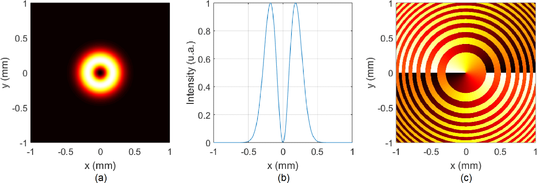
The transverse intensity profile (a and b) and the phase map (c) can be seen in Fig. 1.

Fig. 1
BG beam with TC n = 1., intensity (a and b) and phase map (c) normalized, according to the Eq. 1.

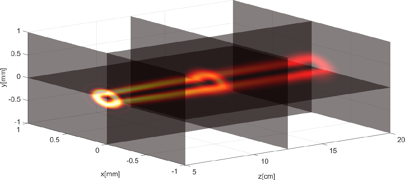
We can see that Fig. 2 shows the displacement of the profile along the z-axis from a certain point, arbitrarily defined.

Fig. 2
Propagation of BG beams with TC n = 1, considering an arbitrary starting point, according to the Eq. 2.

A. Fractional BG Beams

The possibility of dividing the beam’s wavefront into equally spaced parts emerged as an opportunity to utilize the properties of a single optical beam in applications that were previously exclusively restricted to laser behavior. Dividing, or fractionating, a beam or even an optical vortex has become a subject of great scientific study and with great technological applications [³⁵], [³⁶].

In recent years, several techniques have been studied, both in the theoretical field, that is, in the application of mathematical tools that perform beam fractionation, and in the experimental field, in the development of practical techniques to carry out this fractionation. In the first methods to perform the fractionation of these beams, it was common to obtain these beams by defining a fractional (noninteger) value of (n). It was observed that this definition did not provide a description that satisfies the Helmholtz equation or, equivalently, the Maxwell equations [³⁵], [³⁷]. Therefore, an inverse Fourier transform [³⁵] in terms of the order (n) of the beams can be used to obtain the fractional beams. However, there is not only one way to obtain this fractionation, using a Fourier series [³⁶], it is possible to divide the beam into several parts.

In this work, to obtain these fractional BG beams (FBG), we use an inverse Fourier transform in terms of the order (n) of the beams, given by [³⁵], [³⁸].

(3) $$E_{FBG}(r,\theta )=\sum _{l=-\mathrm{\infty }}^{\mathrm{\infty }}{i}^{(n-l)}\frac{\mathrm{sen}[\pi (l-n)]}{\pi (l-n)}{E}_{BG},$$

where l is an arbitrary real number.

The intensity behavior and phase map of an optical beam that has undergone fractionation into 4 parts can be seen in Fig. 3 (a-b) and Fig. 3 (c), respectively. This break in intensity and phase that occurs in the beam allows a new degree of freedom in applications of the same optical beam with the same intensity characteristics [³⁶], [³⁹].

Fig. 3
Characteristics of fractional BG beams with TC n = 3.9, for normalized intensity (a-b) and phase map (c).

It is observed that when the optical beam undergoes this type of fractionation, the wavefront of this beam presents a phase discontinuity, in addition to a low-intensity jump/gap in the laser beam. This phase jump causes a difference of an integer multiple of 2πn [³⁵], in addition to presenting a drop in intensity in the form of a sectioned opening, which characterizes the fractionation of the beam [³⁵], [³⁶].

In the following, we present the generation and analysis process, the experimental results, and the discussion of the transverse and longitudinal intensity and phase properties of these fractionated BG beams using holographic techniques.

III. COMPUTATIONAL HOLOGRAPHIC TECHNIQUES

The holographic technique is a powerful technique for reconstructing the intensity and phase of wavefronts [¹¹]-[¹³], [²⁰], [⁴⁰]. Using computational holographic techniques, it is possible to generate and characterize optical beams with high-quality and experimental precision, particularly non-diffractive optical beams [⁵], [⁷], [¹⁹], [⁴¹], [⁴²].

A. Computer-generated holograms (CGH)

The generation of computer-generated holograms (CGH) is calculated using numerical and computational methods and contains all beam information, which is subsequently implemented in spatial light modulators (SLM) [⁵], [⁷], [¹⁶]-[¹⁹], [⁴¹].

Holographic techniques are widely used in this experimental generation, as they allow individual control of each CGH pixel in real time, in addition to having high quality and experimental fidelity in the reconstruction of the signal sent to the SLM [⁷], [¹⁹], [²¹], [⁴¹], [⁴²].

The CGH is obtained through an amplitude transmission function, varying the reflection coefficient of the SLM based on the following amplitude function [⁷], [⁴²]:

(4) $$H(x,y)=\frac{1}{2}\{\beta (x,y)+\alpha (x,y)\cos [\varphi (x,y)-2\pi (\xi x+\eta y)]\},$$

where β(x, y) = [1 + α²(x, y)]/2, is used to reduce the influence of the beam’s central spectrum, (ξ, η) is the spatial frequency of the reference plane wave, α(x, y) and ϕ(x, y) are the amplitude and phase of the complex beam field [⁷], [¹⁹], [⁴²].

B. Digital Holography

The basic principle of digital holography is the same as that of computer-generated holography, discussed in the previous section. It also consists of two processes: recording and reconstruction process. However, in the recording process in digital holography, the resulting hologram, called a digital hologram, is optical and stored electronically using a CCD (Charged Coupled Device) camera. In the reconstruction process, the digitally stored hologram is numerically reconstructed by a reference plane wave that effectively simulates the reference wave used in the recording process. In this case, the virtual image appears in the position of the original object and the real image is formed, but in the opposite direction of the CCD. For the reconstruction of digital holograms, we consider that the diffraction of a light wave by the aperture or hologram at distance d along the wave propagation direction can be quantitatively described by the Fresnel-Kirchhoff integral [¹⁵], [²⁰]

(5) $$\mathrm{\Gamma }({\xi }^{\prime },{\eta }^{\prime })=\frac{1}{\lambda }{\int }_{-\mathrm{\infty }}^{\mathrm{\infty }}{\int }_{-\mathrm{\infty }}^{\mathrm{\infty }}t(x,y)E_r(x,y)\frac{\exp (-i\frac{2\pi }{\lambda }{\rho }^{\prime })}{{\rho }^{\prime }}dxdy,$$

where t(x, y) is the hologram function ρ^′the distance from a point in the hologram plane to a point in the reconstruction plane. λ is the wavelength used in diffraction, Γ ξ^′ , η^′is the diffracted field in the observation plane, and ρ^′is the distance between a point on the hologram plane and a point on the reconstruction plane, which is given by

(6) $${\rho }^{\prime }=\sqrt{(x-\xi {)}^2+(y-\eta {)}^2+d^2}.$$

The Eq. 5 is the basis of the numerical reconstruction of the hologram, due to which the reconstructed wave field Γ ξ^′ , η^′is a complex function, and both intensity and phase can be calculated. The main advantage of digital holography is that it allows both the optical reconstruction of holograms (using optical beam modulation devices such as SLM, for example [²⁰]) and their numerical reconstruction [⁵], [⁷], [²⁰], [⁴¹].

The computational reconstruction of digital holograms can be done using the angular spectrum method, where A(k_ξ, k_η, z = 0) is the angular spectrum of the obtained hologram. The angular spectrum is defined as the Fourier transform of the digital hologram, i.e.

(7) $$A(k_{\xi },k_{\eta },z=0)=\iint \mathrm{\Gamma }(\xi ,\eta ,z=0)\exp [-i(k_{\xi }\xi +k_{\eta }\eta )]d\xi d\eta ,$$

where k_ξ and k_η are the spatial frequencies of ξ and η, respectively. To calculate the angular spectrum of the beam in z, we must multiply the angular spectrum z = 0 by the factor exp(ik_zz), where $k_z=\sqrt{k^2-k_{\xi }^2-k_{\eta }^2}$. At z = d we have,

(8) $$A(k_{\xi },k_{\eta },z=d)=A(k_{\xi },k_{\eta },z=0)\exp \left(i{k}_{z}d\right).$$

Through the inverse Fourier transform, the field corresponding to this plane is given by,

(9) $$\mathrm{\Gamma }(\xi ,\eta ,d)=\iint A(k_{\xi },k_{\eta },0)\exp \left(i{k}_{z}d\right)\exp \left[i(k_{\xi }\xi +k_{\eta }\eta )\right]d{k}_{\xi }d{k}_{\eta }.$$

The equation 9 results in a matrix of complex numbers and it is possible to determine the amplitude and phase of the object wave using the expressions [⁵], [⁷], [²⁰], [⁴¹];

(10) $$I(\xi ,\eta ,d)=|\mathrm{\Gamma }(\xi ,\eta ,d){|}^2,$$

and,

(11) $$\phi (\xi ,\eta )=\arctan \left[\frac{\mathrm{Im}[\mathrm{\Gamma }(\xi ,\eta ,d)]}{\mathrm{Re}[\mathrm{\Gamma }(\xi ,\eta ,d)]}\right].$$

where φ (ξ, η) is the phase of the object wave.

Thus, it is possible to computationally reconstruct the digital holograms (DH) of the beam using the angular spectrum method using a Fourier transform of the DH [⁵], [⁷], [⁴³]. To compare the experimental results, MatLab software was used to perform simulations, generate CGHs and analyze the optical beam.

C. Experimental setup

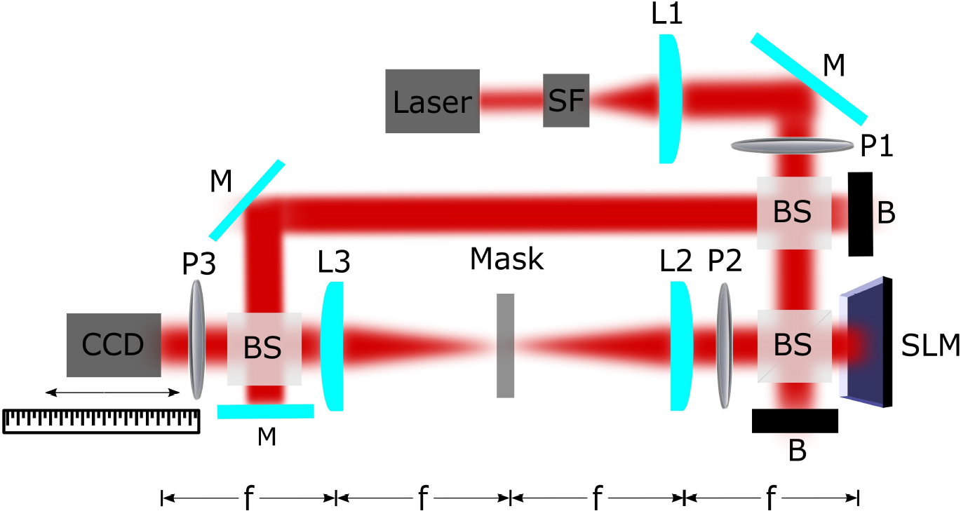
The holographic optical setup is shown in Fig. 4. A He-Ne laser (632.8 nm and 15 mW of Melles Griot power), spatial filter (SF), lenses L1, L2, L3, mirrors (M) and beam splitters (BS) were used. polarizers (P1, P2, P3), a 1280×960 pixel USB CCD camera, model DMK 41BU02.H, from The ImagingSource, with size pixel 4.65 µm [¹³], [¹⁹].

Fig. 4
Configuration of the optical system for holographic technique and interferometric technique; where, lenses (L1, L2, L3), polarizers (P1, P2, P3), beam splitter (BS), spatial filter (SF), mirrors (M), Blocker (B), CCD is the camera, spatiallight modulator (SLM).

An SLM is used to reconstruct the optical beam, allowing greater flexibility in manipulating the system [⁵], [⁷], [²⁰]. The LETO modulator (SLM), from Holoeye Photonics, has a screen resolution of 1920×1080, and a pixel size of 6.4 µm. The display of this modulator allows for the reconstruction of the beam due to the diffraction of light that occurs in the holographic grating of the CGH implemented in the SLM.

Furthermore, this setup is comprised of a 4f Fourier system, which contains two lenses, L2 and L3, at a focal distance of 150 mm, a circular aperture ID (mask), used to identify and choose the first order of diffraction that contains the hologram information.

The digital holography (DH) technique was also used in this work to analyze and characterize the generated optical beams. In this way, an arm with the digital holographic interferometer configuration [⁵], [⁷], [⁴³] was coupled to the beam generation apparatus to obtain holographic interferogram, digital hologram (DH), for analysis of the generated beams. The digital holograms captured in the setup are computationally analyzed using the angular spectrum method already described in the references [⁵], [⁷], [²⁰].

IV. RESULTS

A. Experimental generation of single BG beam

In the hologram generation process (CGH), Eq. 1 and Eq. 4 were used. The wave reference plane was defined with frequency values η = ξ = ∆p/5, where ∆p = 1/δp is the bandwidth, and δp = 6.4 µm corresponds to the size of each individual pixel of the SLM.

For all simulations performed in this work, as well as the experimental results, the values of n = 1 (for integer order BG beams), ω₀ = 256µm, and λ = 632.8 nm were considered. Based on all parameters adopted according to the SLM and also the optical configuration described in Fig. 4. The first results are presented in Fig. 5, where the simulated intensity and phase map can be visualized in Fig. 5 (a and b), and the experimental results obtained through digital holography (DH), intensity and phase map, in Fig. 5 (c and d), respectively.

Fig. 5
Normalized theoretical intensity and phase map (a and b) of BG beams with n = 1, and experimental (c and d), according to CCD parameters.

The experimental intensity observed in Fig. 5 (c) corresponds satisfactorily to what was exposed in the theoretical simulation, showing the formation of the BG beam ring with zero intensity in the center. The phase map obtained experimentally and presented in Fig. 5 (d), is also clearly visible.

The propagation profile of the BG beam along the z-axis, obtained through the arrangement described in Fig. 4 and using the CGH constructed using Eq. 4, is presented in Fig. 6, where Fig. 6 (a) represents the experimental transverse intensity and Fig. 6 (b) the propagation profile. It can be observed that through this experimental arrangement it is possible to obtain a beam propagation of approximately 20 cm, corresponding well to what was simulated and presented in Fig. 2. It is important to mention that every centimeter, a point of displacement, and intensity distribution is captured by the CCD camera.

Fig. 6
Experimentally obtained transverse intensity profile (a) and the propagation (b) at z = 20 cm with n = 1.

In other words, these initial results agree with what was predicted for this beam considering n = 1 and simulated in Fig. 2, where the initial intensity is high, but as the beam propagates on the z axis,the beam loses intensity. Despite this loss of intensity, this beam travels a long distance compared to other optical beams, such as optical vortex generated by other methods.

This first analysis of theoretical and experimental results is in accordance with the predictions described in the literature, presenting satisfactory results. Additionally, the results show that the digital holographic technique is an efficient and applicable technique for this type of analysis of optical beams and vortex.

B. Experimental generation of fractional BG beam

In order to characterize the behavior of the fractionated BG beams, the same method described previously was employed. In this case, considering the fractionation of the beam into distinct parts, the beam was broken into 1, 3, 7 and 9 equally spaced parts.

It is presented in Fig. 7 (a) and (b) the transverse intensity and phase map fractionated with TCn = 0.9 and n = 2.9, while Fig. 7 (c) and (d) presents the experimental transverse intensity and phase map fractionated, respectively. It is possible to observe that in all cases the holographic technique presents satisfactory results in the experimental results of fractional intensity and phase, corresponding to what was theoretically predicted in the computational simulations.

Fig. 7
Normalized intensity and phase map, theoretical (a-b) and experimental (c-d), in according to CCD parameters, for the fractional BG beams with TC n = 0.9 and n = 2.9.

The degree of complexity of the simulated phase maps is much higher compared to that of singlebeam BG, since they are characterized by an asymmetric phase break and are difficult to obtain experimentally.

Despite all the complexity involving phase maps, the DH technique managed to provide good experimental results in relation to fractional beams, presenting phase break in accordance with the theoretical simulation.

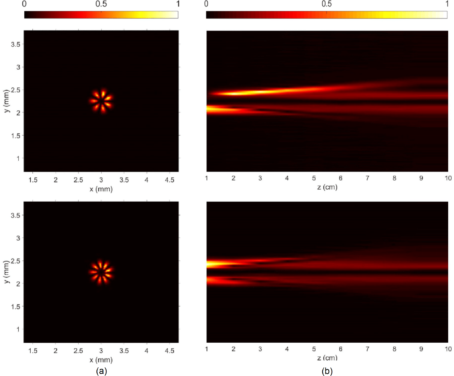
The experimental results of the intensity and longitudinal propagation profile, with TC n = 0.9 and n = 2.9, can be observed in Fig. 8 (a) and (b), respectively.

Fig. 8
BG beam intensity (a) and propagation profile (b) along the z axis, fractionated with TC n = 0.9 and n = 2.9

It is possible to observe that as the fractionation of the beam increases, the lower its intensity willbe; thus, it can be said that its propagation is smaller along the z axis.

The fractional beams observed in Fig. 8 (b) present good experimental results, being well defined and clearly describing the beam displacement.

Furthermore, in order to observe the behavior of this beam in larger fractions, the beam was divided into n = 6.9 and n = 8.9. Thus, in Fig. 9 we present the simulated theoretical results (a-b) and the respective experimental results (c-d) of the phase map and intensity BG beams.

Fig. 9
Normalized intensity and phase map, theoretical (a-b) and experimental (c-d), for the fractional BG beams with TC n = 6.9 and n = 8.9.

We can observe that the greater the fractionation of the beams, the greater the phase break, and the more complex it will be to obtain.

The intensity profiles are in good agreement with the simulations, although the beam dividing lines are narrower compared to the simulation, this is due to the intensity of the laser light applied to generate the beam, as well as the camera resolution and alignment of the beams, in addition to optoelectronic instruments used in holographic interferometry.

The phase maps were analyzed one by one and the best results, presented in Fig. 7 and 9, showthe complexity of working with beams divided into orders greater than 5 parts,due to the asymmetric break in the phase map and also the difficulty in making adjustments to the optical system to obtain these results.

Although its intensity at z = 0 is the same, as the fractionation increases, we observe that the observational quality of the beam decreases, as can be seen in Fig. 10 (a) and (b). Therefore, for practical applications, fractional BG beams of 1 to 5 are more recommended, as they present better experimental propagation results and the intensity and phase profiles are clearly identifiable.

Fig. 10
BG beam intensity (a) and propagation profile (b) along the z axis, fractionated with TC n = 6.9 and n = 8.9.

C. Experimental generation of BG matrices (BGM)

There are many theoretical and experimental works in the literature that investigate the superposition of optical beams or matrices, as presented in references [⁶], [²²], [³²], [⁴⁴], [⁴⁵]. In this present work, we extend this approach to explore the ability to store information about the many BG beams using only one CGH, that is, we create arrays of optical beams and analyze their behavior along the propagation axis, characterizing their intensity, phase map, and displacement profile. Intensity (a-b) and phase map (c) can be seen in Fig. 11 with TC n = 1.

Fig. 11
Normalized intensity (a-b) and phase map (c) for the integer BG beams with TC n = 1.

This approach to BG beams makes it possible to use several optical beams at once without using other experimental apparatus, allowing for increased practical applications in various areas of knowledge, such as optical manipulation, communication systems, or biological physics, as not just a single beam is used, but rather a combination of several beams equally spaced apart.

However, this combination of beams forms a matrix, and its experimental generation will dependon the parameters of the available experimental instruments. Thus, for practical demonstration, in this work 2x2 and 3x3 matrices of the integer BG beams, and 2x2, 3x3 fractionated into 2 and 3 parts were generated in order to compare the integer and fractionated matrices. The Fig. 12 shows the displacement of the simulated BG beam with TC n = 1 along the z axis from a given point, arbitrarily defined.

Fig. 12
Displacement of the simulated BG beam along the z with TC n = 1.

The first simulated (a-b) and experimental (c-d) results of the BG beam matrices can be seen in Fig. 13.

Fig. 13
Normalized intensity and phase map, theoretical (a-b), and experimental (c-d), according to CCD parameters, for the entire BG beams with TC n = 1.

It is possible to observe that the intensity obtained in the experimental result presents a more intense beam ring located in the lower left corner in all matrices; on the other hand, in the upper right corner we observe low light intensity in the beam ring.

This inequality observed in the beam intensity occurs because of the positioning of the experimental apparatus that directs the reference light to the light beam that forms the matrix; in other words, it can be said that this is the result presented by the holographic experimental configuration.

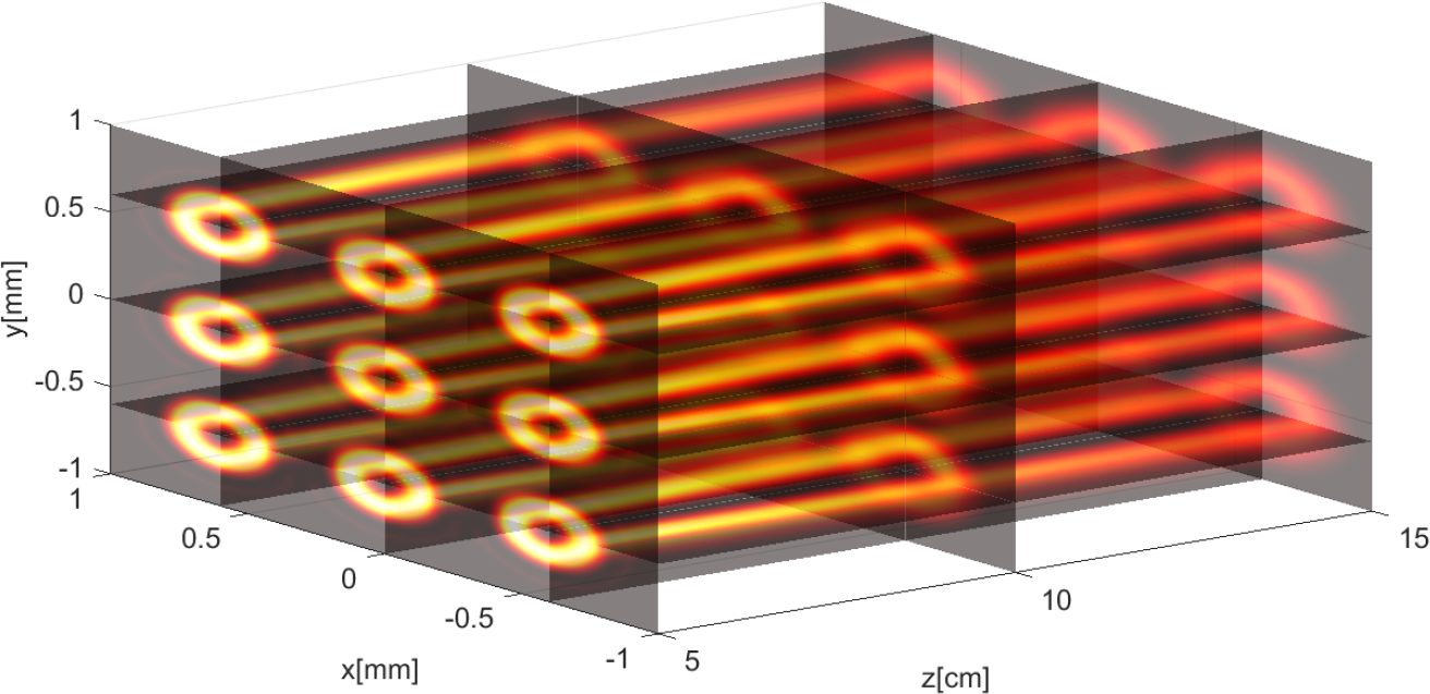
An analysis of the displacement of the BG beam along the z axis was also carried out, as can beseen in Fig. 14, with the transverse intensity (a) and propagation profile (b). This beam propagates more than 20 cm, as shown in Fig. 6 for a single beam.

Fig. 14
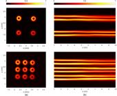
Intensity (a) and propagation profile (b) of the entire BGM beams with TC n = 1 along the z axis at 10 cm.

The experimental intensity results (Fig. 13) are very similar to the simulated theoretical results, with no major beam interference observed that could modify or harm the final result. With regard to the phase results, it is observed that there is also no interference in the field of each beam that could harm the final phase result.

These properties of these beams are extremely interesting and important because, unlike other types of beams where interference effects arise when grouped into matrices, BG beams have shown promise when considering applications with beam matrices.

Regarding the displacement d of the BG beam along the z axis ((Fig. 14), it is observed that the beam loses intensity and presents a small divergence, impairing its propagation over long distances. Therefore, the propagation distance was defined at 10 cm for a perfect visualization of the displacement. The integer BG beams have good beam spacing and their shape does not change at this predefined distance. Furthermore, it is possible to increase the number of beams contained in a single CGH by changing the diameter of the beam so that relevant information such as intensity, phase, and even beam shape is not lost.

D. Experimental generation of fractional BG matrices (BGM)

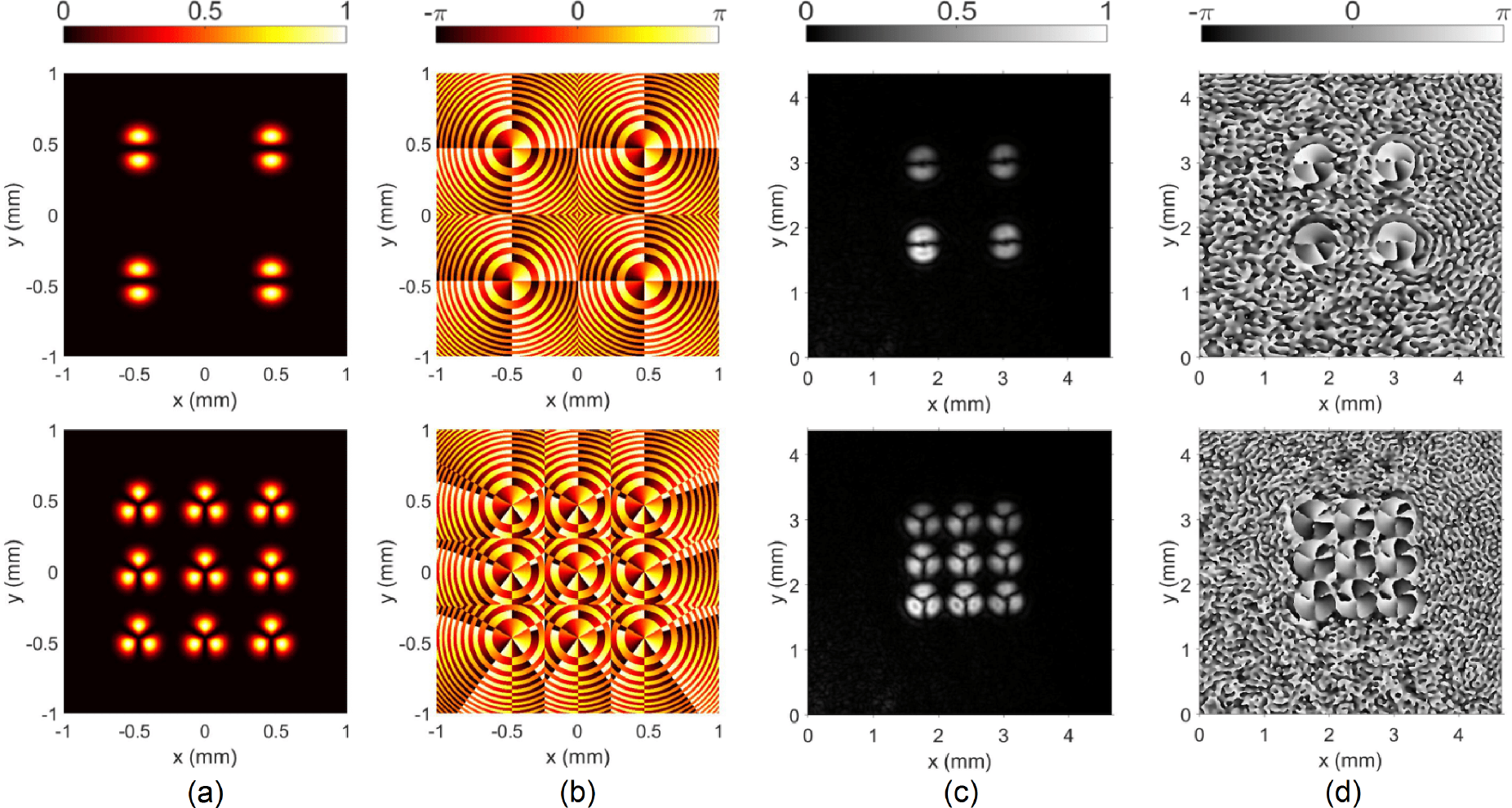
The matrices (2x2 and 3x3) of the fractionated BG beams can be seen in Fig. 15, where some experimental results were selected.

Fig. 15
Normalized intensity and phase map, theoretical (a-b), and experimental (c-d), according to CCD parameters, for fractional BG beams matrices considering 2x2 with TC n = 1.9, and 3x3 with TC n = 2.9.

In Fig. 15 we have the theoretical simulated (a-b) results and also the experimental (c-d) results of the beams divided into 2 and 3 parts, that is, TC n = 1.9 and n = 2.9. We can observe that the theoretical and experimental intensities are clearly distinguishable from each other. Furthermore, proximity of the beams in the 3x3 matrix did not result in interference from the individual fields of each fractionated beam.

The complexity of theoretical phase maps already presupposes that the results of experimental phase maps will be more complex and difficult to obtain perfectly. Although the simulated beams are spatially well separated, the experimental results present very close beams; this is due to the reconstruction of the beam by the holographic interferometry system used to generate the intensity and phase profiles.

A more complex matrix system can be realized with 4x4 or 5x5 matrices; however, the greaterthe number of beams in an optical array, the more complex it will be to obtain phase maps. The experimental results presented satisfactorily correspond to what was theoretically predicted for these matrices.

In order to visualize the best propagation of the fractionated BG beams, it was defined that the displacement distance of the beams would be observed in up to 8 cm, as for higher fractions, the visualization of the beam is compromised. The results of the phase map and beam propagation for larger fractionation do not present satisfactory results. Furthermore, by changing the size of the fractional beam radius, it is also possible to obtain more beams within the matrix, up to the limit of the CCD display resolution.

The intensity and longitudinal propagation profiles were generated for these matrices, as can be seen in Fig. 16 (a) and (b), respectively.

Fig. 16
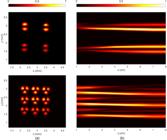
Intensity (a) and propagation profile (b) of the fractional beam matrices considering 2x2 with TC n = 1.9, and 3x3 with TC n = 2.9.

V. CONCLUSIONS

In this work, we present the generation and characterization of integer and fractional Bessel-Gauss beams, as well as integer and fractional BG beam matrices, via holographic techniques. The noveltyof this work lies in the generation of fractional Bessel-Gauss beams, both in the form of a single beam and in the form of matrices, using a computational holographic technique (holograms generated by a computer coupled to a SLM), and, mainly, their characterization using a digital holographic interferometry technique (digital holography with the angular spectrum method) that allows experimentally obtaining a digital hologram and computationally calculating the beam phase distribution. These results for these beams are extremely interesting because, unlike other types of beams where interference effects arise when grouped in matrices, in BG beams these effects are minimal; thus, they have shown to be promising when considering applications with beam matrices. It was observed that the greater the division of the fractional BG beam, the lower its propagation in the optical axis, maintaining its nondiffracting properties in relation to the behavior of an integer BG beam. The experimental results ofall the beams analyzed in this work agree with those predicted in the literature, enabling more precise applications in physical or biological systems, such as optical tweezers or communication systems, and other systems of great scientific and technological interest.

ACKNOWLEDGMENTS

The authors acknowledge financial support from UFABC, CAPES, FAPESP (grant 16/19131-6) and CNPq (grant 302070/2017-6).

REFERENCES

• ^[1] J. J. J. M. Durnin, J. J. Miceli Jr, and J. H. Eberly, “Diffraction-free beams,” Physical review letters, vol. 58, no. 15,pp. 1499-1501, 1987.
• ^[2] L. Allen, M. W. Beijersbergen, R. J. C. Spreeuw, and J. P. Woerdman, “Orbital angular momentum of light and the transformation of laguerre-gaussian laser modes,” Physical review A, vol. 45, no. 11, pp. 8185-8189, 1992.
• ^[3] G. A. Siviloglou, J. Broky, A. Dogariu, and D. N. Christodoulides, “Observation of accelerating airy beams,” Phyical Review Letters, vol. 36, pp. 1760-1765, 2007.
• ^[4] H. E. Hernández-Figueroa, M. Zamboni-Rached, and E. Recami, Localized waves John Wiley & Sons, 2007, vol. 194.
• ^[5] I. S. V. Yepes, T. A. Vieira, R. A. B. Suarez, S. R. C. Fernandez, and M. R. R. Gesualdi, “Phase and intensity analysis of non-diffracting beams via digital holography,” Optics Communications, vol. 437, pp. 121-127, 2019.
• ^[6] M. Zamboni-Rached, “Stationary optical wave fields with arbitrary longitudinal shape by superposing equal frequency bessel beams: Frozen waves,” Optics Express, vol. 12, no. 17, pp. 4001-4006, 2004.
• ^[7] R. A. B. Suarez, A. A. R. Neves, and M. R. R. Gesualdi, “Generation and characterization of an array of airy-vortex beams,” Optics Communications, vol. 458, p. 124846, 2020.
• ^[8] J. K. Jabczyn´ski, “Bessel-gauss coherently combined beams,” Optics Express, vol. 32, no. 6, pp. 10 068-10 076, 2024.
• ^[9] C. H. Acevedo, R. Wu, J. K. Miller, E. G. Johnson, and A. Dogariu, “Colloidal density control with bessel-gauss beams,” Scientific Reports, vol. 11, no. 1, p. 12284, 2021.
• ^[10] M. Cheng, L. Guo, J. Li, and Y. Zhang, “Channel capacity of the oam-based free-space optical communication links with bessel-gauss beams in turbulent ocean,” IEEE Photonics Journal, vol. 8, no. 1, pp. 1-11, 2016.
• ^[11] P.Hariharan, Optical Holography: Principles, techniques and applications, 2nd ed. New York, NY: Cambridge University Press, 1996.
• ^[12] S. A. Benton and V. M. Bove Jr, Holographic imaging, 1st ed. Hoboken, NJ: John Wiley & Sons, 2008.
• ^[13] M. R. R. Gesualdi, “Simplified algorithms of computational holograms: I - for generation of the 3d images,” Revista Brasileira de Ensino de Física, vol. 45, p. e20220244, 2023.
• ^[14] J. M. Webster, “Holographic metrology: some examples of imaging in medicine and non-destructive inspection,” The Imaging Science Journal, vol. 54, no. 2, pp. 80-85, 2006.
• ^[15] U. Schnars and W. Jueptner, Digital Holography: Digital Hologram Recording, Numerical Reconstruction, and Related Techniques, 1st ed. Berlin, GE: Springer, 2005.
• ^[16] C. H. J. Schmitz, K. Uhrig, J. P. Spatz, and J. E. Curtis, “Tuning the orbital angular momentum in optical vortex beams,” Optics express, vol. 14, no. 15, pp. 6604-6612, 2006.
• ^[17] L. Zhu, M. Tang, H. Li, Y. Tai, and X. Li, “Optical vortex lattice: an exploitation of orbital angular momentum,” Nanophotonics, vol. 10, no. 9, pp. 2487-2496, 2021.
• ^[18] Y. Zhang, X. Yang, and J. Gao, “Orbital angular momentum transformation of optical vortex with aluminum metasurfaces,” Scientific Reports, vol. 9, no. 1, pp. 1-9, 2019.
• ^[19] T. A. Vieira, M. Zamboni-Rached, and M. R. R. Gesualdi, “Modeling the spatial shape of nondiffracting beams: Experimental generation of frozen waves via holographic method,” Optics Communications, vol. 315, pp. 374-380, 2014.
• ^[20] I. S. V. Yepes and M. R. R. Gesualdi, “Dynamic digital holography for recording and reconstruction of 3d imagesusing optoelectronic devices,” Journal of Microwaves, Optoelectronics and Electromagnetic Applications, vol. 16, pp. 801-815, 2017.
• ^[21] R. A. B. Suarez, T. A. Vieira, I. S. Yepes, and M. R. R. Gesualdi, “Photorefractive and computational holography inthe experimental generation of airy beams,” Optics Communications, vol. 366, pp. 291-300, 2016.
• ^[22] J. A. V. Mendonça, M. Zamboni-Rached, L. A. Ambrosio, and C. H. d. S. Santos, “Arrays of spatially structured nondiffracting optical beams,” Applied optics, vol. 59, no. 2, pp. 346-353, 2020.
• ^[23] Y. Chen, T. Wang, Y. Ren, Z. Fang, G. Ding, L. He, R. Lu, and K. Huang, “Generalized perfect optical vortices along arbitrary trajectories,” Journal of Physics D: Applied Physics, vol. 54, no. 21, p. 214001, 2021.
• ^[24] P. Li, Y. Zhang, S. Liu, C. Ma, L. Han, H. Cheng, and J. Zhao, “Generation of perfect vectorial vortex beams,” Optics letters, vol. 41, no. 10, pp. 2205-2208, 2016.
• ^[25] M. J. Padgett, J. Molloy, and D. McGloin, Optical Tweezers: methods and applications Boca Raton, FL: CRC press, 2010.
• ^[26] J. Arlt, V. Garcés-Chávez, W. Sibbett, and K. Dholakia, “Optical micromanipulation using a bessel light beam,” Optics communications, vol. 197, no. 4-6, pp. 239-245, 2001.
• ^[27] R. A. B. Suarez, L. A. Ambrosio, A. A. R. Neves, M. Zamboni-Rached, and M. R. R. Gesualdi, “Experimental optical trapping with frozen waves,” Optics Letters, vol. 45, no. 9, pp. 2514-2517, 2020.
• ^[28] R. A. B. Suarez, A. A. R. Neves, and M. R. R. Gesualdi, “Optical trapping with higher-order frozen waves,” Journal of the Optical Society of America B, vol. 40, no. 3, pp. 631-636, 2023.
• ^[29] N. A. Carvajal, C. H. Acevedo, Y. Torres Moreno, et al., “Generation of perfect optical vortices by using a transmission liquid crystal spatial light modulator,” International Journal of Optics, vol. 2017, p. 6852019, 2017.
• ^[30] C. Yang, Y. Lan, X. Jiang, H. Long, J. Hou, and S. Chen, “Beam-holding property analysis of the perfect optical vortex beam transmitting in atmospheric turbulence,” Optics Communications, vol. 472, p. 125879, 2020.
• ^[31] Y. Liu, Y. Ke, J. Zhou, Y. Liu, H. Luo, S. Wen, and D. Fan, “Generation of perfect vortex and vector beams based on pancharatnam-berry phase elements,” Scientific reports, vol. 7, no. 1, p. 44096, 2017.
• ^[32] F. Gori, G. Guattari, and C. Padovani, “Bessel-gauss beams,” Optics communications, vol. 64, no. 6, pp. 491-495, 1987.
• ^[33] V. V. Kotlyar, A. A. Kovalev, and A. P. Porfirev, Vortex laser beams, C. Press, Ed. Boca Raton, Fl: CRC Press, 2018.
• ^[34] M. Anguiano-Morales, M. M. Méndez-Otero, M. D. Iturbe-Castillo, and S. Chávez-Cerda, “Conical dynamics of bessel beams,” Optical Engineering, vol. 46, no. 7, pp. 078 001-078 001, 2007.
• ^[35] H. Zhang, J. Zeng, X. Lu, Z. Wang, C. Zhao, and Y. Cai, “Review on fractional vortex beam,” Nanophotonics, vol. 11, no. 2, pp. 241-273, 2022.
• ^[36] M. Berry, “Optical vortices evolving from helicoidal integer and fractional phase steps,” Journal of Optics A: Pure and Applied Optics, vol. 6, no. 2, p. 259, 2004.
• ^[37] V. V. Kotlyar, A. A. Kovalev, and A. P. Porfirev, “Calculation of fractional orbital angular momentum of superpositions of optical vortices by intensity moments,” Optics express, vol. 27, no. 8, pp. 11 236-11 251, 2019.
• ^[38] C. López-Mariscal, D. Burnham, D. Rudd, D. McGloin, and J. C. Gutiérrez-Vega, “Phase dynamics of continuous topological upconversion in vortex beams,” Optics Express, vol. 16, no. 15, pp. 11 411-11 422, 2008.
• ^[39] J. B. Götte, K. O’Holleran, D. Preece, F. Flossmann, S. Franke-Arnold, S. M. Barnett, and M. J. Padgett, “Light beams with fractional orbital angular momentum and their vortex structure,” Optics express, vol. 16, no. 2, pp. 993-1006, 2008.
• ^[40] A. D. Stein, Z. Wang, and J. S. Leigh Jr, “Computer-generated holograms: A simplified ray-tracing approach,” Computers in Physics, vol. 6, no. 4, pp. 389-392, 1992.
• ^[41] T. A. Vieira, I. S. V. Yepes, R. A. B. Suarez, M. R. R. Gesualdi, and M. Zamboni-Rached, “Optical generation of non-diffracting beams via photorefractive holography,” Applied Physics B, vol. 123, no. 4, pp. 1-10, 2017.
• ^[42] M. R. R. Gesualdi, “Simplified algorithms of computational holograms: II - for generation of the optical beams and vortices,” Revista Brasileira de Ensino de Física, vol. 45, p. e20220248, 2023.
• ^[43] S. Stuerwald, Digital holographic methods Berkeley, CA.: Springer, 2018.
• ^[44] S. H. Tao, W. M. Lee, and X. Yuan, “Experimental study of holographic generation of fractional bessel beams,” Applied optics, vol. 43, no. 1, pp. 122-126, 2004.
• ^[45] S. H. Tao and X. Yuan, “Self-reconstruction property of fractional bessel beams,” JOSA A, vol. 21, no. 7, pp. 1192-1197, 2004.

Publication Dates

• Publication in this collection
  19 May 2025
• Date of issue
  2025

History

• Received
  11 July 2024
• Reviewed
  20 Sept 2024
• Accepted
  24 Mar 2025