Determination of Thermal Process Kinetics by Artificial Neural Networks: A Review Considering Isothermal and Non-Isothermal TG and DSC Data

Abstract

The integration of artificial neural networks (ANNs) with thermal analysis techniques, such as thermogravimetry (TG) and differential scanning calorimetry (DSC), presents great potential to accurately determine kinetics of thermal processes and thermal behavior. This review examines the application of ANNs, including Multilayer Perceptron (MLP) and Hopfield Neural networks (HNN), to analyze both isothermal and non-isothermal TG and DSC data. These networks provide robust tools for predicting thermal behavior, determining kinetic parameters, and modeling complex reaction mechanisms, significantly improving accuracy when compared to traditional methods. The review highlights advances in ANN-based methodologies, including the ability to integrate multiple kinetic models and manage noisy experimental data, thereby offering new insights into thermal decomposition and reaction kinetics. Moreover, the use of HNN in distributed activation energy models (DAEM) is explored, indicating their potential in understanding heterogeneous systems. This study emphasizes the transformative potential of ANNs for improving kinetic studies, suggesting future directions to explore machine learning in material characterization and thermal process optimization.

Keywords:
artificial neural networks; thermal analysis; thermogravimetry; differential scanning calorimetry; kinetics; machine learning

^1.

Introduction

Nowadays, the world is experiencing a new industrial revolution characterized by Artificial Intelligence’s (AI) development and improvement.¹,² Among the various branches of AI, machine learning (ML) stands out, since it can identify patterns in data sets to predict results without relying on pre-programmed instructions.³

Artificial Neural Networks (ANNs) are a type of machine learning algorithm modeled to resemble the biological neural networks found in the brain.⁴ A specific type, called Multilayer Perceptron Neural (MLP) Network, presents a structure consisting of interconnected nodes or artificial neurons arranged in layers that can be trained to perform various tasks. Each node in an ANN receives one or more inputs, performs a calculation, and passes the result on to the next layer of nodes. Nodes in the first layer receive input data, while nodes in the last layer produce the final output of the network.

ANNs have been successfully applied to pattern recognition,⁵ image and speech recognition,⁶,⁷ natural language processing,⁸ automatic control,⁹ financial forecasting¹⁰ among several other applications. They have revolutionized many fields by providing new ways to analyze and understand complex data, and they continue to be an active area of research in machine learning and artificial intelligence.

Thermal analysis is a set of techniques that aims to measure physical properties of a substance and/or its reaction products as a function of time or temperature, when this sample is subjected to a controlled temperature program and under a specified atmosphere.¹¹ This paper will focus on discussing the application of thermogravimetry (TG) and differential scanning calorimetry (DSC), techniques in which the measured physical phenomenon is the variation of mass and heat flux of the sample, respectively, as a function of temperature and/or time.

ANNs can be categorized into three types, based on interpretability: white-box, gray-box, and black-box models.¹²,¹³ White-box models use explicit physical equations. In thermal analysis, an example is the use of kinetic theories applied to extract parameters, such as the triplet kinetic parameters (activation energy, E_a, pre-exponential factor, A, and reaction model), from DSC or TGA data. These models are fully interpretable but struggle with complex, multi-step reactions.¹⁴ Examples of this approach include traditional isoconversional or model-fitting methods.¹⁵,¹⁶ Black-box models are purely data-driven, in which the ANNs model learns input-output patterns without using physical laws.¹⁷,¹⁸ They handle noise and nonlinearity well but lack mechanistic insight and may fail outside their training range.¹⁴

The gray-box model combines both white-box and black-box models. This network architecture integrates traditional modeling with ANNs by optimizing an unknown aspect of the process.² This type of model aims to achieve a balance between interpretability and flexibility but requires high reliability in the parameters and datasets during the training step.

In the last decades, studies¹⁹-²³ have proposed the application of neural networks to determine the values of activation energy, pre-exponential factor, and mechanism. In thermal decomposition processes, the mechanisms are generally complex and not well understood. In addition, to accurately describe the overall process, it is required to assume a combination of several models, constructing the mechanism as a combination of competing, independent, or consecutive steps.²⁴,²⁵

Determining kinetic parameters from experimental data is considered an ill-conditioned inverse problem, which means it may have more than one possible solution.²⁶ The decision about the right (or coherent) solution must be taken together with experimental researchers. It is not an exclusive mathematical issue, from which the best solution is selected by only considering the minimal residual error.

In contrast to thermodynamic quantities, no reference value for E_a can be found in the literature. Consequently, an ANN trained using wrong parameters (or patterns) may fail to learn and correlate correct values in patterns, even if it achieves low adjustment errors during the training step. This step of verifying the parameters can be executed using external methodologies, such as isoconversional analysis for non-isothermal data and Arrhenius analysis for isothermal data.²⁷-²⁹ Also, the experimental conditions must be carefully considered in the ANN thermal behavior prediction,³⁰ as certain materials can present a significant change in the kinetic mechanism depending on the isothermal or non-isothermal process.

Works as the one proposed by Conesa et al.²⁰ simulate data with known kinetic parameters to train the neural network model. This approach is intended to overcome the lack of reference values for E_a. However, there are some points one should be aware of. Taking for example some of the values these authors²⁰ have used for generating the data: the pre-exponential factor k_ref = 5 × 10¹² and E_a/R = 10000. These values yield the product 5e^–10000. However, the same factor in the differential equation to be solved could be achieved by selecting k_ref = 6 × 10¹² and E_a/R = 10000 + ln(6/5). Considering that ln(6/5) ca. 0.18, the change in exponent would be minimal. Thus, one would have certainty only about the rate constant and the model predictions may be biased by the parameter selection. This raises the question: what parameters should be used for simulating the training data? Should all possible combinations be used? If so, how to evaluate the predictions made by the ANN model?

This paper will cover the use of artificial neural networks in two techniques of thermal analysis: TG and DSC. The first works using ANNs were Sbirrazzuoli et al.²³,³¹ for DSC data, Sebastião et al.¹⁹ for isothermal thermogravimetry and Conesa et al.²⁰ for thermogravimetry dynamic data. The objective is to review the leading applications in the field over time and the improvement due to the use of AI for deepening the knowledge in thermal analysis.

^2.

Methodology

^2.1.

Machine learning

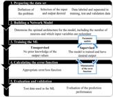
For the successful development of machine learning, it is necessary to have a solid knowledge about the addressed problem and use reliable experimental data, since it is necessary to interpret the results acquired from a good experimental adjustment. These algorithms can be developed in five general steps, as shown in Figure 1.

Figure 1
General steps of ML development.

The choice of the most appropriate machine learning algorithm depends on different factors such as, the physical characteristic of the problem, the number of variables, the mathematical model that best fit the experimental data, among others.³² In thermal analysis, neural networks are commonly applied to investigate thermal behavior, thermal stability and the kinetics of the thermal processes, whether to simulate experimental data or to recover properties.

^2.2.

Neural networks

The artificial neural network (ANN) is a powerful mathematical tool based on the biological communication model, used to solve linear and non-linear problems in various areas of science and has the artificial neuron as its processing unit.³³ These units are arranged in parallel layers, in one or more layers (multilayer perceptron neural network - MLP) or fully interconnected in a recurrent neural network (Hopfield neural network). Neurons communicate unidirectionally through synaptic connections, with their associated weights being adjusted systematically using the steepest descent algorithm, which updates the weights in the direction opposite to the gradient of the error function. The weights optimization process characterizes the training step of the usual neural networks.

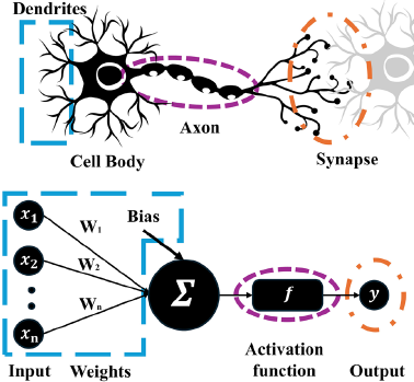
Figure 2 shows a comparison between an artificial neuron and a biological neuron. In a biological neuron, dendrites receive signals from other neurons through synapses. The incoming signal is processed in the soma (cell body) and then sent through the axon, which forms a synapse with the next neuron. In the artificial model, the input layer values act as the external signal, while the synapse is represented by the weights. The processing of this signal, i.e., the summation of the weighted values and the application of an activation function, f, represents the processing that occurs in the cell body. Finally, this processed signal is transmitted to the next set of neurons through synapses, characterized by the next set of weights in the ANN architecture.

Figure 2
Comparison between artificial and biological neurons (adapted from reference 4).

The ANN model was first proposed in 1943 by the neurophysiologist Warren Sturgis McCulloch and the mathematician Walter Harry Pitts Junior.³⁴ In their model, the input data, x_m, together with the synaptic weights w_km are linearly combined by the additive function, equation 1, also considering the bias, b_k. The state of the neurons, u_k, is processed by the activation function f, generating the output y_k, equation 2.⁴

(1)$$u_k=\left({\displaystyle \sum _{j=0}^m{w}_{kj}{x}_j}\right)$$

(2)$$y_k=f(u_k+b_k)$$

The term b_k in equation 2 is the bias, a set of positive or negative external parameters specific to each neuron, designed to increase or decrease the effect of the activation function. The activation function f in equation 2 can assume several mathematical functions depending on the problem. The activation functions used can be monotonically increasing, such as sigmoid or hyperbolic tangent.³⁵

From the literature, in thermal analysis it is observed that Multilayer Perceptron (MLP) network is the most applied to isothermal and non-isothermal TG data and the Hopfield network (HNN) in DSC data. Thus, these two ANN will be discussed in the next sections.

^2.3.

Multilayer Perceptron (MLP) Neural Network

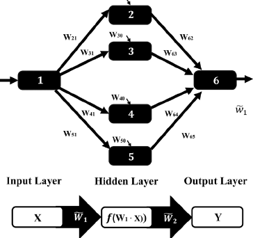
The MLP is a type of network containing successive layers of neurons, enabling it to efficiently tackle complex problems by learning hierarchical representations. Figure 3 schematizes an MLP network with three consecutive layers: the input, one hidden and the output layer.

Figure 3
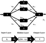
General Multilayer Perceptron Neural Network schematic architecture (adapted from reference 36).

The input data, which can be either experimental data or parameters, is fed into the input layer, as shown in Figure 3, which is commonly activated by a linear function. The information is then transferred to the neurons in the second layer, which are generally activated by a nonlinear activation function, such as tan h(x) or sigmoidal = 1/1 + exp(–xt), depending on the problem. This layer is called hidden or intermediate layer and contains a single or multiple set of neurons. The response of the MLP is determined by the state of the neurons in the output layer, usually calculated as the linear combination of the neuron signals from the previous layer.

The backpropagation algorithm is widely used for supervised training of MLP networks and was proposed in 1986 by Rumelhart and Chauvin³⁷,³⁸ This method is based on the Widrow-Hoff rule or delta rule, which minimizes the error in the output layer by updating the weights of the connections of the previous layers. For this reason, the activation functions used must be continuous and differentiable. The error function, E, to be minimized and the change of network connection weights, Δw_ji, are shown in equations 3 and 4, respectively,⁴

(3)$$E=\frac{1}{2}{\displaystyle \sum _{j=0}^k{(d_i-y_i)}^2}$$

(4)$$\Delta w_{ji}=-\eta \frac{\partial E}{\partial w_{ji}}$$

where k is the number of output neurons in the network, d_i is the desired output and y_i is the output calculated by the network at time t, Δw_ji is the weight change of the connection between neurons i and j, η is the learning rate. When the error function shown in equation 3 represents a minimum value, this will be the acceptable network response.

^2.4.

Hopfield Neural Network

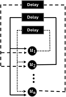
A Hopfield neural network (HNN) is a recurrent single-layer network where all logic units are interconnected. The neurons are connected by a weight factor, Tij,³⁹ between neurons i and j. The neuron state, u_i, is determined by the weighted sum of all neurons connected to it, as well as by external impulses, I_i, represented in equation 5. Figure 4 schematizes a Hopfield network.⁴⁰

Figure 4
General Hopfield Neural Network Architecture (adapted from reference 4).

The neuron state is calculated by the contributions of all other neurons connected to it through a weighted sum of their inputs, as shown in equation 5. However, this contribution is only propagated if the activation function f_j is applied. During the learning time, τ, the information provided to the network is propagated and to maintain the stability of the network and avoid positive feedback, the diagonal elements of the symmetric matrix T_ij are null.⁴¹

(5)$${\mu }_i\frac{d{u}_i(\tau )}{d\tau }=-u_i(\tau )+{\displaystyle \sum _{j=1}^n\left[T_{ij}{\text{f}}_{\text{j}}\left({\text{u}}_{\text{j}}\left(\tau \right)\right)+{\text{I}}_{\text{i}}\left(\tau \right)\right]}$$

In which the factor I_i(τ) represents an external stimulus to the neuron and f_j(u_j(τ) represents the activated state of the neuron. The energy function associated with each state of the network is given by equation 6.

(6)$$E=\frac{1}{2}{\displaystyle \sum _{j=1}^m{e}_j^2}=\frac{1}{2}{\displaystyle \sum _{j=1}^m{\left(C_{cal,j}-C_{\exp ,j}\right)}^2}$$

In which e_j is the difference between C_calc,j, the calculated property and C_exp,j is the experimental property, m is the number of experimental data. A set of differential equations, similar to the Hopfield differential equation 5,⁴² is established by imposing $$\frac{dE}{d\tau }<0$$. The error function expressed by equation 6 can be developed as,⁴³

(7)$$\frac{dE}{d\tau }={\displaystyle \sum _{i=1}^n{\displaystyle \sum _{j=1}^m\left(e_j\frac{\partial (C_{calc,j})}{\partial f_1}\frac{\partial f_i}{\partial u_i}\right)}=\overrightarrow{\nabla }E.\frac{\overrightarrow{df}}{d\tau }<0}$$

Where time-dependence of the neuron state is highlighted. Since $$\frac{dE}{d\tau }>0$$ the condition of minimizing the error function is satisfied if $$\frac{d{u}_i}{d\tau }=-\frac{\partial E}{\partial f}$$ or²⁶

(8)$$\frac{d{u}_i}{d\tau }=-{\displaystyle \sum _{j=1}^m\left(\frac{\partial {(C_{calc})}_j}{\partial f_i}{e}_j\right)}$$

Which validates the minimization of the error function because

(9)$$\frac{dE}{d\tau }=-{\displaystyle \sum _{j=1}^n\left(\frac{\partial f_i}{\partial u_i}{\left(\frac{\partial u_i}{\partial \tau }\right)}^2\right)<0}$$

It is important to note that the HNN error function is a monotonically decreasing function, i.e., the neuron states will converge to the nearest stable point, where $$\frac{d{u}_i}{d\tau }=0$$. Consequently, the initial conditions used when solving these equations will influence the accuracy of the solution. Therefore, having a solid understanding of the underlying chemistry and physics of the problem is crucial.

The integration of equation 8 is commonly performed by numerical methods, as for example the fourth-order Runge-Kutta method.

^3.

Thermal Analysis

Thermal analysis can be used in a wide range of applications in chemistry and engineering,²⁷ such as characterization of materials,⁴⁴,⁴⁵ determination of thermal stability,⁴⁶,⁴⁷ investigation of kinetic mechanisms in thermal decomposition processes,⁴⁸ pyrolysis⁴⁹ and determination of adsorption parameters.⁵⁰

The temperature control of the experiments can be set as isothermal, T = const, or non-isothermal, T = T(t). Usually, the non-isothermal condition is programmed by linear heating rate, β = dT/dt = const, called dynamic condition.¹⁶ This review will focus on thermogravimetry (TG) using isothermal and non-isothermal experiments and differential scanning calorimetry (DSC) with dynamic data.

For kinetic study, experimental data, i.e., mass loss for TG and heat flux for DSC, is converted to degree of conversion, α, which is adopted in the general kinetic equation¹⁵

(10)$$\frac{d\alpha }{dt}=k(T)f(\alpha )$$

in which

(11)$$\alpha =\frac{m_0-m_i}{m_0-m_f}(TG)or\alpha \frac{{\text{H}}_i}{\Delta \text{H}}(DSC)$$

with m₀, the initial mass, m(t), mass along the process, m_f, final mass for TG. And H_i as the partial area calculated at time i and ∆H as the total area of the DSC signal. The rate constant, k(T), is usually given by the Arrhenius equation,²⁹

(12)$$k(T)=A\exp \left(-\frac{Ea}{RT}\right)$$

with A being the pre-exponential factor (usually in s^-1 or min^-1), E_a, the activation energy (usually in kJ mol^-l) and R, the universal gas constant (8.314 J K^-1 mol^-l).

Rearranging equation 10 for dynamic condition, β = dT/dt = const, the general kinetic equation is represented as,

(13)$$\beta \frac{d\alpha }{dT}=k(T)f(\alpha )$$

In a conventional approach, equation 13 can be fitted using individual kinetic models, f(α), presented in Table 1. These models are proposed to describe the physical phenomenon and are grouped into 3 classes of curve profiles: acceleratory, deceleratory, and sigmoidal (or autocatalytic).¹⁵

Table 1
Kinetic models established in the literature for thermal decomposition processes¹⁵,¹⁶

Model	Symbol	f(α)	g(α)
Reaction order
Zero-order	F1/R1	1	α
First-order	F1	(1 – α)1	−ln(1 − α)
Second-order	F2	(1 – α)2	[1/(1 – α)] – 1
Third-order	F3	(1 – α)3	(1/2)[(1 – R)–2 – 1]
Nucleation
Avrami-Erofeev n = 2	Am2	2(1 – α)(–ln(1 – α)1/2	[−ln(1 − α)]1/2
Avrami-Erofeev n = 2	Am3	3(1 – α)(–ln(1 – α)2/3	[−ln(1 − α)]1/3
Avrami-Erofeev n = 4	Am4	4(1 – α)(–ln(1 – α)3/4	[−ln(1 − α)]1/4
Geometric contraction
Contracting cylinder	R2	2(1 – α)1/2	1−(1 − α)1/2
Contracting sphere	R3	3(1 – α)2/3	1−(1 − α)1/3
Diffusion
1D	D1	1/(2α)	α2
2D	D2	–[1/ln(1 – α)]	((1 – α)ln(1 – α)) + α
3D: Jander model	D3	[3(1 – α)2/3]/[1 – (1 – α)1/3]	(1 − (1 − α)1/3)2
3D: Ginstling-Brounshtein model	D4	3/[2((1 – α)–1/3 – 1)]	1 − (2/3)α − (1 − α)2/3
Power law
Power Law n = 2	P2	2α1/2	α1/2
Power Law n = 3	P3	2α2/3	α1/3
Power Law n = 4	P4	4α3/4	α1/4

By solving equation 13, it is possible to obtain the kinetic triplet, i.e., activation energy, E_a, pre-exponential factor, A, and the kinetic model, f(α), or its integrated function, g(α).⁵¹ The A and E_a parameters can be determined by isoconversional methods,²⁸,⁵²-⁵⁴ generally called model-free methods, since no kinetic model is assumed in this approach.⁵⁵

According to the International Confederation for Thermal Analysis and Calorimetry (ICTAC), the kinetics study by isoconversional methods must be performed using at least three TG curves with different β values.¹⁵ Depending on the sample, the thermal event can occur through multiple steps with competing or consecutive reactions.⁵⁶ Thus, it is necessary to use robust methodologies to clarify the physical phenomena.² This work will highlight the use of neural networks to solve this chemical problem.

^4.

Artificial Neural Network Applied to Isothermal TG Data

Sebastião, Braga, and Yoshida¹⁹ developed a multilayer neural network model using published experimental data for rhodium acetate. For the input, it was adopted isothermal TG curves at the temperatures 198, 202.5, 203.5, 205.0, 207.0, 209.0 and 210.5 °C.

In this work,¹⁹ it is proposed to replace the usual activation functions used in the MLP models by the kinetic model. Thus, equation 10 can be rewritten for constant temperature, K(T) = k(s^–1) as

(14)$${\displaystyle {\int }_0^{\alpha }\frac{d\alpha }{f(\alpha )}=g(\alpha )=kt+k_0}$$

In their paper, the first order equation was used, thus the activation function for the hidden layer was defined as

(15)$$\text{α(t)=1}-e^{kt+k_0}$$

The first model studied in their paper¹⁹ was using a single neuron in the hidden layer. By using data at different temperatures and plotting the predicted k values against 1/T it was possible to calculate the pre-exponential factor and activation energy, assuming the rate constant as the Arrhenius factor.

By increasing the number of neurons, prediction improvement was observed up to 8 neurons and after that it was observed overfitting of data. In this first work, the same activation function was applied to all neurons and the authors mentioned the loss of physical meaning if more than one neuron is considered.

Since the model is predicting the rate constant, k, rather than the pre-exponential factor, A, and activation energy, E_a, the results are less likely to be affected by multiple parameter combinations that yield equivalent mass loss. This issue will be discussed in the next section.

Based on the model discussed above, Sebastião et al.³⁶ developed a MLP network with a different algorithm to optimize the error function. The first step of the algorithm consists of fixing the interconnection weights between input and intermediate layers. For this, the experimental data is fitted by the individual kinect models, from Table 1, g(α) = kt + k₀. The rate constant and linear coefficients will be represented by the interconnection weights and bias, respectively. The additive function, representing the state of neurons in the hidden layer, is determined as

(16)$$W_{1}X=\left(\begin{array}{c}{\text{w}}_{21}\text{t}+{\text{w}}_{20}\\ {\text{w}}_{31}\text{t}+{\text{w}}_{30}\\ {\text{w}}_{41}\text{t}+{\text{w}}_{40}\\ {\text{w}}_{51}\text{t}+{\text{w}}_{50}\end{array}\right)$$

with X as the state of neuron in the input layer, receiving the time data and the values w_i1 and w_i0 correspond to the values of the rate constants k and k₀ for the kinetic models, respectively. Therefore, there is a physical meaning for the interconnection weights and biases in this model.

In the second stage of the algorithm, a non-linear transformation is performed, in which each neuron in the intermediate layer is activated. However, in this algorithm, each neuron in this layer is activated by a different activation function, f, corresponding to the kinetic models presented in Table 1, as

(17)$$B=f(W_{1}X)$$

The mathematical functions used in this work to activate the neurons were the Prout-Tompkins and the Avrami-Erofeev models, with m = 2, 3 and 4, described in Table 1. Thus, the neurons in the intermediate layer of the proposed MLP network are represented in equation 16. It is important to note that this network structure is not rigid, allowing the addition of other kinetic models, as well as the exclusion of some models depending on the system under study.

(18)$$f\left(W_{1}X\right)=\left(\begin{array}{c}Au\left({\text{w}}_{21}\text{t}+{\text{w}}_{20}\right)\\ A{m}_2\left({\text{w}}_{31}\text{t}+{\text{w}}_{30}\right)\\ A{m}_3\left({\text{w}}_{41}\text{t}+{\text{w}}_{40}\right)\\ A{m}_4\left({\text{w}}_{51}\text{t}+{\text{w}}_{50}\right)\end{array}\right)$$

Each neuron in the intermediate layer is pondered by the weights in the output layer W₂. The vector W₂ can be exemplified as

(19)$$w_2={(w_{62}{w}_{63}{w}_{64}{w}_{65})}_{1X4}$$

In the third stage, a linear transformation is performed to determine the state of the neuron in the output layer, Y, consisting in a linear combination of the neurons in the hidden layer, as

(20)$$Y=w_{2}f(W_{1}X)$$

The error of the MLP network is defined considering the difference between experimental data and calculated property by the network as

(21)$$E=\left|\right|Y_{cal}-Y_{\exp }|{|}_2^2,\text{\hspace{0.17em} \hspace{0.17em} being }{Y}_{cal}=W_{2}f(XV)$$

with this network structure it is possible to calculate the contribution of the various kinetic models used in the process through a Levenberg-Marquart optimization,

(22)$$w_2={\left(B^{\text{T}}B\right)}^{-1}{B}^T{Y}_{cal}$$

It is interesting to note that this algorithm stands out from the others because it is a robust mathematical method in the study of thermal decomposition, since it uses the rate constants as fixed weights of the network, enabling the convergence of the network to a coherent physical result, in addition to considering the contribution of several models in the process. Therefore, this algorithm becomes useful for studying thermal decomposition of different systems. By comparing the error of the individual model adjustments with the MLP model, it was observed an increase in the adjustment by a factor of 2-7, which proves that the best description of the process is given by the combination of models rather than an individual mechanism.

This same algorithm was adopted in the MLP network developed by Ferreira et al.⁵⁷ on the study of anti-human immunodeficiency virus (HIV) drugs: efavirenz (EFV) and lamivudine (3TC), where it was added the kinetic models of acceleration (E potential law), deceleration (geometric model, linear, area and volume contraction), diffusion (one, two, three dimensions and Ginstling-Brounshtein). For this MLP, 13 neurons were used in the intermediate layer and the state of the neurons in the intermediate layer can be determined by

(23)$$f\left(w_{i}x\right)=\left(\begin{array}{l}{f}_{D_1}(W_{2_1}t+W_{2_0}\\ f_{D_2}(W_{3_1}t+W_{3_0}\\ f_{D_3}(W_{4_1}t+W_{4_0}\\ f_{D_4}(W_{5_1}t+W_{5_0}\\ f_{R_1}(W_{6_1}t+W_{6_0}\\ f_{R_1}(W_{7_1}t+W_{7_0}\\ f_{R_3}(W_{8_1}t+W_{8_0}\\ f_{A_2}(W_{9_1}t+W_{9_0}\\ f_{A_3}(W_{{10}_1}t+W_{{10}_0}\\ f_{A_4}(W_{{11}_1}t+W_{{11}_0}\\ f_{F_1}(W_{{12}_1}t+W_{{12}_0}\end{array}\right)$$

In the EFV network, for the input, it was used experimental TG curves at temperatures 172, 173, 174, 175 and 178 °C. For the output, the kinetic parameters of activation energy, E_a = 75.230 kJ mol^–1 and pre-exponential factor, A = 3.2190 × 10¹⁶ s^–1 were also determined by applying the Arrhenius analysis. The residual error of adjustment by the network is on average 10³ times lower compared to the best individual kinetic model: R1. In the 3TC study, for the input, it was used experimental TG curves at the temperatures 215, 220, 223, 225, 228, 230, 237, 240 and 250 °C. For the output, the kinetic parameters of activation energy, E_a = 103.25 kJ mol^–1 and pre-exponential factor, A = 2.5587 × 10^-3 s^–1. The residual error of adjustment over the network is on average 10² times lower compared to the best individual kinetic model: D4.

This algorithm was also used in Ferreira at al.⁵⁸ with thalidomide, in which the MLP network also had 13 kinetic models in the intermediate layer. The activation energy determined by the network was compared with the activation energies determined along the process by the isoconversional methods of Friedman,⁵² Vyazovkin,⁵⁴ and Kissinger-Akahira Sunose⁵³ with non-isothermal experimental data. The isothermal TG curves at temperatures 293, 304, 314, and 324 °C were used, and the best individual kinetic model was the R2 model, with the error of, on average, 10⁵ times higher compared to the residual error of adjustment over the network. The MLP dealing with isothermal data presented the activation energy for the entire process of 98.94 kJ mol^-1. For the non-isothermal analysis, it was used four heating rates: 2.5, 5.0, 10 and 20 °C min^-1 in N₂ atmosphere and the activation energy were calculated as 98-108 kJ mol^-1 along the process.

Ferreira et al.⁵⁹ used this MLP in the study of automotive polyurethane, in which two neural networks were proposed, one being composed of eleven kinetic models and the other composed of only the Rn and Dn models, which were chosen because these models offered smaller residual error. The activation energies determined by the network were compared with those determined by the Friedman,⁵² Vyazovkin,⁵⁴ and Kissinger-Akahira Sunose⁵³ methods with non-isothermal experimental data. The isothermal data were performed at temperatures 380, 390, 400 and 410 °C and the MLP results indicated a two-step process, in which the first occurs from the beginning until 40% of conversion, described by contraction of active nuclei, model R3, followed by diffusion, D4. The MLP adjustment of the experimental data was, on average, 10² to 10³ times more accurate than the best individual kinetic model. It presented the activation energy for the entire process of 184.2 kJ mol⁻¹ considering the diffusion model D4 and 198.7 kJ mol⁻¹ for the contraction model. For the non-isothermal analysis, it was used four heating rates 2.5, 5.0, 10 and 20 °C min^-1 in N₂ atmosphere, and the activation energy was calculated as 188.9 and 186.8 kJ mol⁻¹, respectively determined by the isoconversional methods Flynn-Wall-Ozawa⁵³ (FWO) and Kissinger-Akahira Sunose (KAS)⁵³ at 40% of conversion and 193.7 and 191.6 kJ mol⁻¹ at extension of 60-70% of conversion.

It is important to note the necessity of adjusting each individual kinetic model before defining it as the activation function for the ANN. If these parameters are to be freely optimized while comparing the sum of different models against experimental data, different combinations of rate constants for different models could lead to the error functions with the same order of magnitude, making it difficult to evaluate which parameters have the most appropriate physical meaning.

^5.

Artificial Neural Network Applied to Non-Isothermal TG Data

Conesa, Caballero and Reyes-Labarta²⁰ developed a multilayer neural network model to predict the kinetic constants using pre-exponential factor, k_ref, activation energy, E_a, and reaction order, n. The model receives input simulated patterns of TG curves with 20 experimental data in each curve, calculated at different heating rates. The ANN has one hidden layer and one output layer, consisting of three neurons, one for each parameter. To generate the training data, the following reaction for pyrolysis was considered

(24)$$F\underrightarrow{pyrolisis}(1-s)G+sG$$

with F being the fraction of the sample to decompose, G the gas produced during the process, S the solid residue and s the solid fraction remaining after the process has been completed. Then, the reaction speed can be determined using the global weight loss, w, as

(25)$$\frac{dw}{dt}=-k_{ref}{F}^n(1-s)e^{\frac{E_a}{R}\left(\frac{1}{T}\frac{1}{T_{ref}}\right)}$$

with R the ideal gas constant. The authors mentioned that the following values were used to generate the data set: 1, 5 and 8 min^-1 for k_ref; 10000, 15000, 20000, 30000 and 35000 K for $\frac{E_a}{R}$; 0.5, 1, 2 and 2.5 for n. This produced a set of 60 curves. However, it is not clear the values they have used for the heating rates, F, T_ref and s while generating the training data.

For training the model with theoretically calculated values, the authors splitted the data into different subsets, one for training (used for updating the model weights) and validation (to evaluate the model performance on unseen data during the training procedure). They have used two different approaches to avoid overfitting: (i) regularization, which applies a penalty to the error function if large weights are used during the training; (ii) early stopping, which stops the training procedure if the validation data error starts increasing. They determined that 10 neurons were used in the input layer for the regularization approach and 4 for the early stopping, both using sigmoid as the activation function. In the trained model, it is not clear which one of the two models mentioned, was able to retrieve the constants in agreement with the values acquired using other methods while using experimental data for cellulose, polyethylene and lignin. It is emphasized by the authors that the model is specific for systems that can be modeled by single n^th-order reactions.

Caution must be taken while simulating data with pre-selected E_a and ^ref values for training an ANN model. In equations such as (equation 25), the factor $K(T)=-k_{ref}{e}^{\frac{E_a}{R}\left(\frac{1}{T}\frac{1}{T_{ref}}\right)}$ may have the same value for different combinations of k_ref and E_a, this is known as kinetic compensation effect.⁶⁰

Therefore, the parameter selected may bias the model predictions when applying it to experimental data. Although this procedure does not allow for a straightforward evaluation of the predicted individual parameters, the final value for K(T) is likely to be the same for all model predictions. Different combinations of parameters that lead to the same similar exponential factor have been also observed for another problem.⁶¹

Therefore, if the objective is to determine the rate constant for the reaction, ANN models would offer more reliability, as discussed in the section 4. However, if the objective is obtaining E_a and k_ref, that should be done using isoconversional or Arrhenius analysis and using the neural network for making other predictions. If ANN models are used to predict these parameters, they should be trained on a dataset containing multiple experimental curves where the values for these parameters were obtained through the analysis mentioned previously. This approach ensures that the model learns from real data, enhancing the reliability of its predictions.

ANN can be used to model different properties of a material and provide insights about its formulation. Burgaz et al.¹⁷ investigate the use of artificial neural networks (ANNs) to predict the thermal stability, crystallinity, and thermomechanical properties of different proportions of poly(ethylene oxide) (PEO) and clay nanocomposite compositions. The proportions obtained and simulated were PEO – n% clay, with n = 0, 5, 10, 15, 20, and 100. The authors trained different ANNs for each type of experimental data: thermogravimetric analysis (TGA), DSC, and dynamic mechanical analysis (DMA). All input data were normalized using the normalization equation,

(26)$${\text{x}}_{\text{n}}=\frac{\text{x}-{\text{x}}_{\min }}{{\text{x}}_{\max }-{\text{x}}_{\min }}(highlimit-lowlimit)+lowlimit$$

with x_min and x_max the minimum and maximum values of experimental data. High and low limits are defined as 1 and 0, respectively. All neural networks used the feed-forward back propagation algorithm. The data was splitted into training (75%), validation (15%), and testing (15%) sets. For DMA neural networks, one hidden layer was enough to predict the storage modulus (E’) and tan δ (the ratio of the loss modulus (E’’) to the storage modulus (E’)) using 193 training data for each case. For TGA data, a neural network was necessary to have two hidden layers to predict weight loss using 406 training data. For DSC data, one hidden layer was used to predict the heat flow using 565 training data. The results demonstrate the potential of ANNs for predicting different properties of polymer/clay nanocomposites. The training process revealed that increasing the amount of data enhances the network’s modeling capacity. In DMA analysis, the relationship between the storage modulus and temperature is much less nonlinear compared to relations between the input and output parameters in both DSC and TGA. Thus, the modeling capability of ANN is the highest for the DMA analysis. Therefore, the authors increased the number of hidden layers to improve the accuracy for TGA and DSC data. An option broadly discussed to improve the accuracy in modeling thermal data is the use of more than one heating rate, which could be another possibility for the performance enhancement in this work, as can be seen in ICTAC.²⁵,²⁷ The neural networks developed in this work do not provide information about the kinetic parameters and mechanisms for the experimental data.

Muravyev and Pivkina¹³ proposes the application of ANNs for predicting kinetic parameters from simulated thermoanalytical data. The input data consisted of conversion degree versus temperature profiles (α(T)) generated for single and multiple heating rates, as well as constant-rate thermal analysis (CRTA) runs. The output included the kinetic triplet (activation energy E_a, pre-exponential factor log A , and reaction model f(α)) with ANNs trained on a broad range of parameters (E_a = 50 – 300 kJ mol^–1, log A = 0.01 – 40 s^–1) and 10 reaction models.

Key findings demonstrate that ANNs, particularly multilayer perceptrons, achieve high accuracy (performance > 99% for some models) in predicting kinetic parameters, outperforming traditional single-heating-rate methods. Advantages of the ANN approach include rapid analysis, tolerance to noisy data, and adaptability to complex kinetic scenarios. However, limitations were noted for single-heating-rate inputs (low predictive power outside training ranges) and simultaneous prediction of multiple parameters (reduced accuracy). The work underscores ANNs as a promising alternative to conventional kinetic methods. A critical point highlighted was that the simulated data considered was single-step reactions, considering that greater computational power is required to work with multi-step reactions.

In reference,¹³ a broad range of parameters selection for generating the data set is a good practice, since it increases the amount of data for training the model. The authors mentioned the kinetic compensation effect while trying to determine the kinetic triplet in the usual methods and that, hypothetically, using ANN would result in lower parameter interdependency. However, the kinetic compensation effect may still be a problem while generating the simulated data. For all combinations of pre-exponential factors and activation functions considered, it would be good to have an analysis of the set of parameters that would produce the same reaction rates. Thus, although the model had an excellent performance, the evaluation of these parameter predictions remains a challenge.

Rojek, Suchacz, and Wesolowski⁶² proposed performing incompatibility detection between active pharmaceutical ingredients (API) and excipients based on thermogravimetric data using a self-organization map (SOM). In this work, binary mixtures of caffeine and selected excipients were used as a study model.

The SOM network can be applied for clustering, feature extraction and anomaly detection. It will map higher dimensional data into a lower dimensional grid. In this type of model, the input data is passed to a grid of interconnected neuros and one of these will be promoted to an activated state. Thus, similar data will activate neurons close to each other.

The input data for this model is a discrete set of temperatures corresponding to a percentage of mass loss, from 5% (T₅) up to 75% (T₇₅) in increments of 5%. To appropriately map the data, different models consisting of 2D grids were tested, 3 × 3, 4 × 4, 5 × 5 and 6 × 6, and the 5 × 5 grid was found to be the optimal for this problem.

After training the model, the weight values of the neuron connections were used to perform a principal component analysis (PCA) and cluster analysis (CA) to identify the temperature of mass loss which would potentially indicate incompatibility. The predictions of the model were compared against DSC, Fourier transform infrared spectroscopy (FTIR) and powder X-ray diffraction (PXRD). It was found that DSC and FTIR agreed with the predictions and that the range of temperatures potentially most important for indicating incompatibility are those corresponding to mass losses from 20 to 55%.

Therefore, this result indicated that ANNs combined with thermogravimetry can be used as a diagnostic tool to determine incompatibility occurrence between (API) and excipients.

Özge Çepelioğullar et al.⁶³ applied ANNs to predict refuse-derived fuel (RDF) pyrolytic behaviors. The model proposed in their study consists of one input layer that receives temperature and heating rate data, two hidden layers and an output layer that predicts the weight loss at that temperature.

The data was generated using 7 different heating rates: 5, 10, 15, 20, 30, 40 and 50 °C min^-1. For each parameter it was recorded approximately 4000 datapoints. From this data set, the optimal number of 1000 points to be selected at random was acquired by trial and error. From the selected data, 75% was used for training, 15% for testing and 15% for validation steps. The training process was carried out for different combinations parameters: number of neurons in the hidden layer varying from 3 to 7, giving a total of 25 possible combinations; activation functions used in the hidden layer were tan-sigmoidal or log-sigmoidal, giving a total of 4 different combinations; each model was trained 5, 10 and 25 times, which gives 3 different combinations. Thus, in total, there were 100 different models trained 3 times each. The best performance was observed for the model trained 25 times, containing 7 and 6 neurons in the first and second hidden layers, with tan-sigmoidal or log-sigmoidal activation functions, respectively.

In their work,⁶³ the model was able to predict the data with high accuracy for all training, test and validation sets. The model was used to predict a new TG curve generated with a heating rate of 25 °C min^-1 and the predictions were very accurate while comparing against experimental data. This work makes evident the importance of the model design step. It is important to note at this point that a good and generalizable model should be able to predict data within the limits of the data used for the training step, in this case for heating rates of 5 and 50 °C min^-1 and minimum/max temperatures. The authors highlight the effectiveness of ANNs in capturing the complex thermal decomposition characteristics of RDF, suggesting their potential as powerful tools for reducing the number of TG experiments needed.

Monticeli et al.⁶⁴ uses an artificial neural network to predict thermal degradation curves for four different fibers: ramie, curaua, kenaf and jute. While describing the ANN approach, it is mentioned the Conesa et al.²⁰ work and described a process for data acquisition assuming the same n^th order kinetic reaction given by equation 25. However, there is no further mention to this theoretical dataset in the text.

The model proposed in their work⁶⁴ receives as inputs the time, temperature and heating rate. It has 12 hidden layers and outputs the prediction for the mass loss. The data set was acquired experimentally with temperature ranging from 25 to 800 °C and using heating rates of 5, 10, 20 and 40 °C min^-1.

The authors⁶⁴ started the ANN model training by first considering only one heating rate, 10 °C min^-1, and they separated the data into training and test sets and the method performance was evaluated based on the determination coefficient of the test set. The number of data to be used in the training step was determined by evaluating the model performance for all four fibers for different numbers of training data. However, it is not clear the total number of data nor what percentage the number of training data represents. They have observed that as the number of training data increases, the performance for all fibers analyzed converged to the same value for number of training data of 60. Without knowing what percentage this number represents, it is hard to evaluate this selection as appropriate or not. The regression plots presented for comparing predicted and target values shows an excellent agreement.

After describing the training process, it is said that the same procedure was performed for the other heating rates, to achieve an ANN model capable of prediction data at heating rates not accessed experimentally. However, it is not clear what procedure the authors have used: did they use transfer learning for each one of the other heating rates? Or did they retrain the model using all data at the same time using the hyperparameters determined in the first step? The performance for unseen heating rates is demonstrated by showing a plot for the three-dimensional TG surface having 5 and 40 °C min^-1 as lower and upper limits.

Still regarding the training step, in the conclusion section the authors said only one heating rate was used to train the model. This seems to contradict the description in the results section.

Araujo et al.⁶⁵ investigated the application of MLP neural networks to the biopolymer chitosan’s TG dynamic data. The authors aim to demonstrate the effectiveness of MLP neural networks in modeling the kinetics of solid thermal decomposition. For the chitosan experimental data, the MLP shows the lowest residual error to fit experimental data, which were performed at N₂ atmosphere under four heating rates: 2.5, 5.0, 7.5, and 10 °C min^-1. The activation energy was calculated as 98.1 to 183.3 kJ mol^–1 along the conversion degree. The findings show that MLP neural networks provide a robust and accurate tool for understanding the complex decomposition behaviors of biopolymers, enhancing the predictive capability for thermal analysis in various industrial applications. This methodology has been applied to different materials’ thermal decomposition, for example, graphene oxide,²² nitroxides,⁶⁶ and Eu³⁺-betadiketonate coordination compounds.⁶⁷

The model architecture is based on the isothermal neural network proposed by Sebastião et al.,³⁶ and follows the same development discussed in the section 4. The innovation consists of adding neurons in the input layer, representing the temperature for each conversion degree in different heating rates, β. Also, another difference is the interconnection weights between the intermediate and input layers, which are determined assuming,

(27)$$W_1(T_{\alpha i})=\left(\frac{A}{\beta }\frac{R}{E_{\alpha }}{T}^2\exp \left(\frac{E_{\alpha }}{R{T}_{\alpha i}}\right)\right)$$

with the activation energy and pre-exponential factor determined using the isoconversional method.²⁸,⁵⁴ The kinetic models presented in Table 1 also activate the hidden layer, thereby ensuring not only the optimization of the neural network but also preserving the physical significance of the weights.

De Freitas-Marques et al.⁶⁸ also applied the MLP neural network proposed above for the kinetic studies of the drugs atazanavir sulfate (ATA) and ritonavir (RIT) thermal analyses. The thermal behavior of ATA indicates melting at 190.7 °C (ΔH_m = 71.5 J g⁻¹) with decomposition (E_a = 101.8 kJ mol^–1). For RIT indicates melting at 119.2 °C (ΔH_m = 66.5 J g⁻¹) with decomposition (E_a = 100 kJ mol^–1; α = 10%). The kinetic model that contributes the most is the Avrami-Erofeev model with m = 2 and describes the thermal decomposition of ATA and RIT. The MLP model for atazanavir was trained using the heating rate curves at 14, 18, and 20 °C min^-1. It was shown that the kinetic parameters, E_a, A, and the kinetic contribution model retrieved for the MLP neural network were able to recover an experimental curve at 40 °C min^-1. It demonstrates the capability of the proposed neural network to extrapolate experimental data.

Araujo et al.⁵⁶,⁶⁹ explored using the HNN to model kinetic behaviors and activation energy distribution in complex systems. For this approach, it is assumed that several reactions may occur in the same event and the activation energy, for the whole process, is described by a probability density function, f(E_a), instead of an average value, where each reaction has its probability in the process, P(E_a). For this, the experimental data can be represented as,

(28)$$(1-\alpha )={\displaystyle \sum P({\text{E}}_{\text{a}})}{e}^{-{\displaystyle \int \frac{k}{\beta }dT}}$$

The probability function is determined by $P(E_a)=\frac{aV}{V*}={\displaystyle {\int }_{E_a}^{E_a+d{E}_a}f(E_a)d{E}_a}$. The integral can be further developed as ${\displaystyle \int f}(E_{ai})d{E}_a={\displaystyle \sum f}(E_{ai})={\displaystyle \sum \frac{P(E_{ai})}{\Delta (E_{ai})}\Delta (E_{ai})}$, in which the Δ(E_ai is a convenient range of E. Considering a continuous distribution of activation energy and also the probability density function, f(E_a) = P(E_a)/∆(E_a), the equation 28 can be rewritten as equation 29 and can be interpreted as the first-order integral Fredholm equation,

(29)$$(1-\alpha )={\displaystyle \sum _{i=1}^n{w}_i{\displaystyle {\int }_0^{\infty }K(T,E_a)f_i(E_a)d{E}_a}}$$

with K(T, E) the kernel and f(E_a) the activation energy distribution function. This equation represents a class of problems known as ill-posed inverse problem, and the HNN approach, tested with both simulated and experimental data, demonstrates better efficiency compared to the traditional methods, offering a promising tool for thermal analysis in industrial applications. Araujo et al.⁵⁶,⁶⁹ used the HNN to estimate kinetic parameters in the distributed activation energy models (DAEM). This method can estimate the shape of f(E) without a priori assumption of its functional form, and a constant pre-exponential factor, A. For training the model, simulated data with random noise was performed. For the kinetic model determination, the HNN algorithm was adapted to obtain the parameters of the Cai-Liu model, f(α) = αm(1 – qα)n. In addition, their model was robust to noise in the experimental data.

Wakimoto et al.⁷⁰ proposed an improvement for the method proposed by Araújo et al.,⁵⁶ the new methodology estimates the kinetic parameters in the DAEM without a priori assumption of both f(E_a) and the pre-exponential factor A. The model was tested by performing a kinetic analysis on reaction data of the parallel reaction system generated by numerical simulations under seven heating conditions in which N is the reactions proceed in parallel, and the data can be written as,

(30)$$(1-\alpha )={\displaystyle {\sum }_i^N\frac{V_i^{*}}{V_i}\exp \left[-\exp \left(-\ln \frac{\beta }{T^2}-\frac{E_{ai}}{RT}+\ln \frac{A_{i}R}{E_{ai}}\right)\right]}$$

where V_i*/V_i denotes the contribution of the i^th reaction. The estimation of conversion α, can be regarded as the forward propagation of the three-layer neural network and the kinetic parameters A_i, E_ai, and V_i*/V_i can be obtained as the optimized weights and biases of this neural network.

For that, $\frac{\beta }{{\text{T}}^2}$ and 1/T are the input to the neural network and are normalized by Z-score normalization⁷¹ to prevent a negative influence of the input variables on the optimization using the gradient descent method and the loss function to be minimized is defined by,

(31)$$(objecive)=\frac{1}{M}{\displaystyle {\sum }_{j=1}^M{(X_j-X_{\exp ,j})}^2+\lambda \left|\left({\displaystyle {\sum }_{j=1}^N\frac{V_i^{*}}{V_i}-1}\right)\right|}$$

where X_exp is the experimental value of conversion and M, the number of data points. The first term in equation 31 is the mean squared error (MSE), and the second term is used to constrain the sum of V_i*/V* to unity, with λ = 0.1 being a coefficient that balances the first and second terms.

The limitation of the proposed method is the determination of the hyperparameters in the neural network. The proposed method has several hyper-parameters, and optimizing all of them requires too much computational cost. In this study, the authors changed the lower limit of V_i*/V* , and fixed the other hyperparameters. The number of hidden layer nodes in the neural network (i.e., the number of reactions proceeding in parallel) was set to N = 64. The possible range of E_a was limited to 0.1-10000 kJ mol^–1. The initial activation energy of each reaction was set randomly in E_a = 0.1-400 kJ mol^–1. For the gradient descent method, the number of optimization steps was set to 10⁵.

^6.

Artificial Neural Network Applied to DSC Data

For the DSC analysis, Sbirrazzuoli and Brunel²³ showed the mechanism for homogeneous kinetic processes as f(α_i) = (1 – α_i)ⁿ is appropriate for many systems.³¹,⁷² Assuming the equation 10, whit α_i = H_i/∆H being determined from H_i, as the partial area calculated at time i, and ∆H as the total area of the DSC signal, one has

(32)$${\left(\frac{dH}{dt}\right)}_i=\Delta H\cdot A{e}^{-\frac{E_{\alpha }}{R{T}_i}}\cdot f({\alpha }_i)$$

in which the DSC experimental data of heat flow is P_i = (dH_i/dt). By taking the logarithm in equation 32, we can establish the general equation,⁷³,⁷⁴

(33)$$\ln \left[{\left(\frac{dH}{dt}\right)}_i\left(\frac{1}{\Delta H}\right)\right]-n\ln (1-{\alpha }_i)=\ln A-\frac{E_a}{R{T}_i}$$

Sbirrazzuoli and Brunel²³ were the first to propose using artificial neural networks for filtering and deconvoluting calorimetric signals.³¹ Their study utilized synthetic thermoanalytical curves of heat flow relative to temperature, with the objective function being the difference between the synthetic data, Y_r,i,exp and the recovered curve Y_r,i,cal as

(34)$$E={\displaystyle \sum _{r=1}^M\frac{1}{N}{\displaystyle \sum _{i=1}^N{\left(Y_{r,i,\exp }-Y_{r,i,cal}\right)}^2}}$$

with N as the number of recorded points and M as the number of patterns. The aim of the study was to evaluate the ability of neural networks to determine thermodynamic and kinetic parameters from DSC curves.

The training data was simulated by solving equation 33 assuming f(α_i) = (1 – α_i)ⁿ, with n = 2, activation energy ranging from 74 to 80 kJ mol^–1 and ln(A) ranging from 18 to 20. These values were based on previous experimental results for the reaction of interest. In reference 23, the authors mentioned that after generating the data, the kinetic parameters and enthalpy are computed using the single peak method. In reference 31, it seems the values used as target were those used for simulating the data, without carrying out the parameter recovery step.

The optimal topology for their ANN model was determined as receiving 320 input values, representing the DSC curve, having three hidden layers with 15, 20 and 20 neurons and outputting the results for ∆H, E_a and ln(A). For the training step, the authors used the resilient-propagation algorithm²³ to optimize the model weights. The total number of curves to be used for training the model was evaluated by carrying out the process for different steps for E_a and ln(A). Also, noise was added to the training input data to assess the model capability to learn and sensibility to noisy data as input.

The authors in reference 31 found that the model was able to recover the parameters used for simulating the curves with good accuracy with both clean and noisy data. Demonstrating that ANN models are potential useful tools for thermal analysis.

It is interesting to note that for their work, the range of values used for generating the data is based on previously determined experimental results. That potentially makes the model prediction more reliable. Also, the model was not applied to experimental data for making predictions. If that was the case, it is always important to note that using simulated data for training a model makes it difficult to assess if the model is learning physically meaningful trends or artifacts due to parameter correlations, as discussed previously about the kinetic compensation effect. The authors also mentioned about the possibility of finding different combinations of parameters corresponding to low errors while using single-peak methods.⁷⁵

Considering another strategy, equation 2 was treated by Hopfield neural network-based algorithm by Sebastião and co-workers⁷⁶ to determine the kinetic parameters m and n as the reaction order, E_a the activation energy, and A the pre-exponential factor. A general kinetic model f(α) = α^m(1 – qα)ⁿ was considered, in which the mechanism depending on the m, n and q parameters, describing the physics and chemistry of the process.³⁰,⁷³

The Hopfield neural network-based algorithm used the equation 26 as the multi objective error function and to investigate the performance of the algorithm to fit DSC data and compute the kinetic parameters. It was used 1000 synthetic data of dH/dt(T), for each heating rate, and to each case it was incorporated random errors of 2.5% point-by-point in the Y_r,i,exp synthetic curves. It was observed that the HNN method is not sensitive to noisy data.

Experimental data of an antihypertensive drug, losartan potassium, LOK, during its polymorphic conversion were investigated.⁷⁶ It was assumed

(35)$$rmsd={\displaystyle \sum _{r=1}^3\sqrt{\frac{{\displaystyle {\sum }_{i=1}^N{\left({\left(\frac{dH}{dt}\right)}_{r,i(calc)}-{\left(\frac{dH}{dt}\right)}_{r,i(\exp )}\right)}^2}}{N}}}$$

with rmsd as the root mean square deviation and three heating rates of DSC data in a multi objective error function. From the results, it was stated the LOK conversion presented A = 6.376 × 10¹² s^–1, E_a = 136.5 kJ mol^–1, m = 0.6, n = 0.85 and q = 1.0. Therefore, it is observed that the process occurs as a combined event, once the values of these parameters in the f(α) function do not correspond to any ideal kinetic model.

When using the HNN method, it is important to keep in mind that the method converges to the nearest stable solutions. Therefore, when defining the initial guess to the set of Hopfield different equations, it is important to have a good estimate of the values for the real process. Additionally, using simulated data is not an issue, as it does not rely on training with a dataset before being applied to experimental data.

In this work, the authors have tested different initial conditions while applying the method to experimental data and found different sets of parameters that lead to small residuals. In that case, since all parameters were physically acceptable, the set with smaller residual was selected as the final answer.

^7.

Conclusion

This review highlights the potential of artificial neural networks (ANNs) in analyzing and interpreting thermal analysis data, specifically TG and DSC. A table with the papers discussed is available in the Supplementary Information section. The application of ANNs, with emphasis on the MLP and HNN, has significantly enhanced the accuracy and complexity of kinetic analyses for both isothermal and non-isothermal processes. By integrating simulated and experimental data with robust computational algorithms, these networks provide a powerful framework for predicting thermal behavior, characterizing kinetic parameters, and modeling complex reaction mechanisms. The findings demonstrate that ANN-based methodologies surpass traditional optimization algorithms like Levenberg-Marquardt in adaptability and robustness, being able to handle noise in experimental data and complex multi-step reaction processes.

However, some caution must be taken while conducting studies in this field. For models such as MLP, that rely on a training data set, using simulated data during the training step previously to the application to experimental data, for predicting kinetic parameters, may introduce bias in the model predictions, as different combinations of pre-exponential factor and activation energy can lead to the same result. For training these models, ideally it should be used an extensive experimental dataset from which the kinetic parameters were extracted from other methods, as, for example, the isoconversional analysis. As for the HNN, it is important to have a good initial guess for the problem solution to prevent the method from converging to a minimum on the error surface that corresponds to non-physical parameters. The existence of multiple minima on the error surface can also be an issue for MLP models. Therefore, it is important to train and test the model with the chosen topology using multiple different initialization for weights and biases to ensure that the topology can learn the problem effectively, regardless of its initial parameters.

Future work should explore the broader applicability of these methodologies to diverse materials and conditions. Additionally, advances in machine learning architectures and training algorithms can possibly provide further improvement of its predictive capabilities and computational efficiency of ANNs in thermal analysis. The integration of these technologies represents a paradigm shift, bridging experimental thermal analysis with computational intelligence to unlock new possibilities in materials science and engineering.

Supplementary Information

Supplementary data are available free of charge at http://jbcs.sbq.org.br as PDF file.

Acknowledgments

The authors would like to thank Conselho Nacional de Desenvolvimento Científico e Tecnológico (CNPq), process 05870/2023-8, Fundação de Amparo à Pesquisa do Estado de Minas Gerais (FAPEMIG), Coordenação de Aperfeiçoamento de Pessoal de Nível Superior, Brazil (CAPES) for financial support, Programa de Pós-graduação em Química da UFMG (PPGQUI-UFMG) and Programa de Pós-graduação em Inovação Tecnológica da UFMG (PPGIT-UFMG).

Author Contributions

Rita C. O. Sebastião was responsible for the conceptualization, writing original draft, review and editing, project administration; Natália R. S. Araujo for the conceptualization, writing original draft, review and editing; Felipe S. Carvalho for writing-review and editing; Bárbara D. L. Ferreira for the conceptualization and writing original draft; João Pedro Braga for writing-review and editing.

Rita C. O. Sebastiãois a full professor at Universidade Federal de Minas Gerais (UFMG) with experience in Chemistry, working mainly on the topics: inverse problems, artificial neural networks, nuclear magnetic resonance, thermal decomposition of solids, chemical kinetics, combustion processes, and thermodynamics. Extensive experience in education, research, and extension, especially in projects aiming for the popularization of science, educational innovation, and entrepreneurship, connecting the university to basic education. Experience in developing and managing projects on socio-environmental sustainability and education. She is currently a member of the Postgraduate Program in Chemistry, Postgraduate Program in Technological Innovation and Professional Master’s in Technological Innovation and Intellectual Property at UFMG.

Natália R. S. Araujo is a PhD candidate in Chemistry at Universidade Federal de Minas Gerais, where she also earned her Bachelor’s and Master’s degrees. She has experience in Physical Chemistry, focusing on the development of MLP and Hopfield neural networks, combustion kinetics, and thermal decomposition kinetics. Her research includes theoretical chemistry and thermal analysis.

Felipe S. Carvalho earned his bachelor’s in Chemistry from Universidade Federal de Viçosa and his MSc and PhD in Theoretical Chemistry from Universidade Federal de Minas Gerais. His research interests include inverse problems, chemical kinetics, adsorption, deep learning applied to physical chemistry, and statistical thermodynamics of liquids. As a research scholar at California State University, Northridge, he contributed to 3D-RISM method development in AmberTools: including CUDA acceleration, ionic parameter optimization and a water placement package. Currently, he is a research scholar at the California Institute of Technology, studying molecular dynamics of polymers at water-surface interface.

Bárbara D. L. Ferreira is Bachelor (2010) in Chemistry from the Universidade Federal de Viçosa. Master (2012) and Doctor (2016) in Chemical Sciences from the Universidade Federal de Minas Gerais. Specialist in Higher Education (2020) and Chemistry Teaching (2021) from Claretiano Centro Universitário (2020). She has postgraduate degree in Teacher Training for EaD (2020) and Educational Design (2020) from CEFOR-Training Center of Instituto Federal do Espírito Santo. She has experience in Physical Chemistry, ill-conditioned inverse problems, Hopfield artificial neural network and MLP, combustion kinetics, thermal decomposition kinetics, nuclear magnetic resonance and image reconstruction on computed tomography.

João Pedro Braga holds a degree in Chemistry (1979), a master’s degree in Physics (1982) both from the Federal Universidade Federal de Minas Gerais (UFMG), a PhD in Chemistry from the University of Sussex (1986) and a Visiting Fellow position at Princeton University (1996). He is currently a full professor (retired) at UFMG. He has published seven books (Physical Chemistry, Quantum Chemistry, Statistical Thermodynamics, Marie Curie’s visit to Brazil, Maria Sklodowska-Curie W Brazylii, Statistical Thermodynamics/second edition, Numerical Methods in Quantum Chemistry) and spent thirty-seven years as a productivity fellow at CNPq. Professor Braga has experience in the area of Physical Chemistry.

References

• ¹ Malik, S.; Muhammad, K.; Waheed, Y.; Ain Shams Engineering J. 2024, 15, 102886. [Crossref]
  » Crossref
• ² Muravyev, N. V.; Luciano, G.; Ornaghi, H. L.; Svoboda, R.; Vyazovkin, S.; Molecules 2021, 26, 3727. [Crossref]
  » Crossref
• ³ Jordan, M. I.; Mitchell, T. M.; Science 2015, 349, 255. [Crossref]
  » Crossref
• ⁴ Haykin, S.; Neural Networks: A Comprehensive Foundation, 3^rd ed.; Prentice-Hall, Inc.: Upper Saddle River, NJ, 2007.
• ⁵ Durodola, J. F.; Li, N.; Ramachandra, S.; Thite, A. N.; Int. J. Fatigue 2017, 99, 55. [Crossref]
  » Crossref
• ⁶ Hossain, M. A.; Rahman, M. M.; Prodhan, U. K.; Khan, M. F.; arXiv:1308.3785 2013 [Crossref]
  » Crossref
• ⁷ Świetlicka, I.; Kuniszyk-Jóźkowiak, W.; Świetlicki, M.; Sensors 2022, 22, 321. [Crossref]
  » Crossref
• ⁸ Goldberg, Y.; Neural Network Methods for Natural Language Processing; Morgan & Claypool: Toronto, 2017. [Crossref]
  » Crossref
• ⁹ Cho, B. C.; Liaw, S.-L.; Chang, C.-N.; Yu, R.-F.; Yang, S.-J.; Chiou, B.-R.; Water Sci. Technol. 2001, 44, 95. [Crossref]
  » Crossref
• ¹⁰ Kaastra, I.; Boyd, M.; Neurocomputing 1996, 10, 215. [Crossref]
  » Crossref
• ¹¹ Brown, M. E.; Gallagher, P. K.; Handbook of Thermal Analysis and Calorimetry: Recent Advances, Techniques and Applications, vol. 5; Elsevier: Amsterdam, 2011.
• ¹² Rudin, C.; Nat. Mach. Intell. 2019, 1, 206. [Crossref]
  » Crossref
• ¹³ Muravyev, N. V.; Pivkina, A. N.; Thermochim. Acta 2016, 637, 69. [Crossref]
  » Crossref
• ¹⁴ Galván, I. M.; Zaldívar, J. M.; Hernández, H.; Molga, E.; Comput. Chem. Eng. 1996, 20, 1451. [Crossref]
  » Crossref
• ¹⁵ Vyazovkin, S.; Burnham, A. K.; Criado, J. M.; Pérez-Maqueda, L. A.; Popescu, C.; Sbirrazzuoli, N.; Thermochim. Acta 2011, 520, 1. [Crossref]
  » Crossref
• ¹⁶ Khawam, A.; Flanagan, D. R.; J. Phys. Chem. B 2006, 110, 17315. [Crossref]
  » Crossref
• ¹⁷ Burgaz, E.; Yazici, M.; Kapusuz, M.; Alisir, S. H.; Ozcan, H.; Thermochim. Acta 2014, 575, 159. [Crossref]
  » Crossref
• ¹⁸ Al-Yaari, M.; Dubdub, I.; Polymers 2020, 12, 1813. [Crossref]
  » Crossref
• ¹⁹ Sebastião, R. C. O.; Braga, J. P.; Yoshida, M. I.; J. Therm. Anal. Calorim. 2003, 74, 811. [Crossref]
  » Crossref
• ²⁰ Conesa, J. A.; Caballero, J. A.; Reyes-Labarta, J. A.; J. Anal. Appl. Pyrolysis 2004, 71, 343. [Crossref]
  » Crossref
• ²¹ Vieira, S. S.; Paz, G. M.; Araujo, B. C. R.; Lago, R. M.; Sebastião, R. C. O.; Thermochim. Acta 2020, 689, 178628. [Crossref]
  » Crossref
• ²² Menezes, I. R. S.; Araújo, N. R. S.; Araújo, B. C. R.; Sakai, T.; Lago, R. M.; Sebastião, R. C. O.; Thermochim. Acta 2023, 721, 179454. [Crossref]
  » Crossref
• ²³ Sbirrazzuoli, N.; Brunel, D.; Neural Comput. Applic. 1997, 5, 20. [Crossref]
  » Crossref
• ²⁴ Koga, N. In Handbook of Thermal Analysis and Calorimetry, vol. 6, 2^nd ed.; Elsevier: Amsterdam, 2018, ch. 6. [Crossref]
  » Crossref
• ²⁵ Vyazovkin, S.; Burnham, A. K.; Favergeon, L.; Koga, N.; Moukhina, E.; Pérez-Maqueda, L. A.; Sbirrazzuoli, N.; Thermochim. Acta 2020, 689, 178597. [Crossref]
  » Crossref
• ²⁶ Braga, J. P.; Lemes, N. H. T.; Borges, E.; Sebastião, R. C. O.; Quim. Nova 2016, 39, 886. [Crossref]
  » Crossref
• ²⁷ Koga, N.; Vyazovkin, S.; Burnham, A. K.; Favergeon, L.; Muravyev, N. V.; Pérez-Maqueda, L. A.; Saggese, C.; Sánchez-Jiménez, P. E.; Thermochim. Acta 2023, 719, 179384. [Crossref]
  » Crossref
• ²⁸ Vyazovkin, S.; J. Therm. Anal. 1997, 49, 1493. [Crossref]
  » Crossref
• ²⁹ Vyazovkin, S.; Wight, C. A.; Thermochim. Acta 1999, 340-341, 53. [Crossref]
  » Crossref
• ³⁰ Vyazovkin, S.; Chrissafis, K.; Di Lorenzo, M. L.; Koga, N.; Pijolat, M.; Roduit, B.; Sbirrazzuoli, N.; Suñol, J. J.; Thermochim. Acta 2014, 590, 1. [Crossref]
  » Crossref
• ³¹ Sbirrazzuoli, N.; Brunel, D.; Elégant, L.; J. Therm. Anal. 1997, 49, 1553. [Crossref]
  » Crossref
• ³² Mahesh, B.; Int. J. Sci. Res. 2020, 9, 381. [Crossref]
  » Crossref
• ³³ Wu, Y.; Feng, J.; Wireless Pers. Commun. 2018, 102, 1645. [Crossref]
  » Crossref
• ³⁴ McCulloch, W. S.; Pitts, W.; Bull. Math. Biophys. 1943, 5, 115. [Crossref]
  » Crossref
• ³⁵ Apicella, A.; Donnarumma, F.; Isgrò, F.; Prevete, R.; Neural Networks 2021, 138, 14. [Crossref]
  » Crossref
• ³⁶ Sebastião, R. C. O.; Braga, J. P.; Yoshida, M. I.; Thermochim. Acta 2004, 412, 107. [Crossref]
  » Crossref
• ³⁷ Chauvin, Y.; Rumelhart, D. E.; Backpropagation: Theory, Architectures, and Applications; Lawrence Erlbaum Associates: Hillsdale, New Jersey, USA, 1995.
• ³⁸ Suliman, A.; Zhang, Y.; J. Earth Sci. Eng. 2015, 5, 52. [Link] accessed in May 2025
  » Link
• ³⁹ Hopfield, J. J.; Proc. Natl. Acad. Sci. 1982, 79, 2554. [Crossref]
  » Crossref
• ⁴⁰ Hopfield, J. J.; Proc. Natl. Acad. Sci. 1984, 81, 3088. [Crossref]
  » Crossref
• ⁴¹ Hopfield, J. J.; Tank, D. W.; Biol. Cybernetics 1985, 52, 141. [Crossref]
  » Crossref
• ⁴² Lemes, N. H. T.; Borges, E.; Braga, J. P.; J. Braz. Chem. Soc. 2007, 18, 1342. [Crossref]
  » Crossref
• ⁴³ Sebastião, R. C. O.; Lemes, N. H. T.; Virtuoso, L. S.; Braga, J. P.; Chem. Phys. Lett. 2003, 378, 406. [Crossref]
  » Crossref
• ⁴⁴ Silva, C. R. G.; Fialho, S. L.; Barbosa, J.; Araújo, B. C. R.; Carneiro, G.; Sebastião, R. C. O.; Mussel, W. N.; Yoshida, M. I.; de Freitas-Marques, M. B.; J. Braz. Chem. Soc. 2021, 32, 638. [Crossref]
  » Crossref
• ⁴⁵ Peñalver, R.; Arroyo-Manzanares, N.; López-García, I.; Hernández-Córdoba, M.; Chemosphere 2020, 242, 125170. [Crossref]
  » Crossref
• ⁴⁶ Reda, S. Y.; Ciência e Tecnologia de Alimentos 2011, 31, 475. [Crossref]
  » Crossref
• ⁴⁷ Yan, Q.-L.; Zeman, S.; Elbeih, A.; Thermochim. Acta 2012, 537, 1. [Crossref]
  » Crossref
• ⁴⁸ L’vov, B. V; Thermochim. Acta 2002, 386, 1. [Crossref]
  » Crossref
• ⁴⁹ Slopiecka, K.; Bartocci, P.; Fantozzi, F.; Appl. Energy 2012, 97, 491. [Crossref]
  » Crossref
• ⁵⁰ Senthil Kumar, P.; Senthamarai, C.; Durgadevi, A.; Environ. Prog. Sustainable Energy 2014, 33, 28. [Crossref]
  » Crossref
• ⁵¹ Schick, C.; Vyazovkin, S.; Koga, N.; Handbook of Thermal Analysis and Calorimetry, vol. 6, 2^nd ed.; Elsevier: Amsterdam, 2018. [Crossref]
  » Crossref
• ⁵² Friedman, H. L.; J. Polym. Sci. B 1969, 7, 41. [Crossref]
  » Crossref
• ⁵³ Mothé, C. G.; de Miranda, I. C.; J. Therm. Anal. Calorim. 2013, 113, 497. [Crossref]
  » Crossref
• ⁵⁴ Vyazovkin, S.; Dollimore, D.; J. Chem. Inf. Comp. Sci. 1996, 36, 42. [Crossref]
  » Crossref
• ⁵⁵ Arenas, C. N.; Navarro, M. V.; Martínez, J. D.; Bioresour. Technol. 2019, 288, 121485. [Crossref]
  » Crossref
• ⁵⁶ Araújo, N. R. S.; Duarte, Á.C. M.; Pujatti, F. J. P.; Freitas-Marques, M. B.; Sebastião, R. C. O.; Thermochim. Acta 2021, 697, 178847. [Crossref]
  » Crossref
• ⁵⁷ Ferreira, B. D. L.; Araujo, B. C. R.; Sebastião, R. C. O.; Yoshida, M. I.; Mussel, W. N.; Fialho, S. L.; Barbosa, J.; J. Therm. Anal. Calorim. 2017, 127, 577. [Crossref]
  » Crossref
• ⁵⁸ Ferreira, B. D. L.; Araújo, N. R. S.; Ligório, R. F.; Pujatti, F. J. P.; Mussel, W. N.; Yoshida, M. I.; Sebastião, R. C. O.; J. Therm. Anal. Calorim. 2018, 134, 773. [Crossref]
  » Crossref
• ⁵⁹ Ferreira, B. D. L.; Araújo, N. R. S.; Ligório, R. F.; Pujatti, F. J. P.; Yoshida, M. I.; Sebastião, R. C. O.; Thermochim. Acta 2018, 666, 116. [Crossref]
  » Crossref
• ⁶⁰ Koga, N.; Šesták,J.; Thermochim. Acta 1991, 182, 201. [Crossref]
  » Crossref
• ⁶¹ Carvalho, F. S.; Braga, J. P.; Alves, M. O.; J. Mol. Model. 2022, 28, 286. [Crossref]
  » Crossref
• ⁶² Rojek, B.; Suchacz, B.; Wesolowski, M.; Thermochim. Acta 2018, 659, 222. [Crossref]
  » Crossref
• ⁶³ Çepelioğullar, Ö.; Mutlu, İ.; Yaman, S.; Haykiri-Acma, H.; J. Anal. Appl. Pyrolysis 2016, 122, 84. [Crossref]
  » Crossref
• ⁶⁴ Monticeli, F. M.; Neves, R. M.; Ornaghi Jr., H. L.; Cellulose 2021, 28, 1961. [Crossref]
  » Crossref
• ⁶⁵ Araujo, N. R. S.; Sebastião, R. C. O.; Freitas-Marques, M. B.; da Nova Mussel, W.; Yoshida, M. I.; Virtuoso, L. S.; Therm. Sci. Eng. Prog. 2022, 36, 101490. [Crossref]
  » Crossref
• ⁶⁶ França, C. S.; Porto, D. L.; Junior, J. H. S.; Souza, F. S.; Nascimento, T. G.; Nogueira, F. H. A.; Gomes, A. P. B.; Jordão, A. K.; Ribeiro, E. H. S.; Araújo, N. R. S.; Sebastião, R. C. O.; Aragão, C. F. S.; J. Therm. Anal. Calorim. 2022, 147, 13395. [Crossref]
  » Crossref
• ⁶⁷ Queiroz, E. C.; Marques, L. F.; Carvalho, G. R.; Gomes, E. M.; Franco, D. F.; Quirino, W. G.; Rodrigues, J. S. M.; Freire, R. O.; Freitas-Marques, M. B.; Araújo, N. R. S.; Yoshida, M. I.; Sebastião, R. C. O.; Pinheiro, C. B.; Machado, L. O. M.; Machado, F. C.; Opt. Mater. 2024, 154, 115672. [Crossref]
  » Crossref
• ⁶⁸ de Freitas-Marques, M. B.; Araújo, N. R. S.; Rosa Jr., A. A.; Yoshida, M. I.; de Oliveira Sebastião, R. C.; da Nova Mussel, W.; J. Therm. Anal. Calorim. 2024, 149, 7329. [Crossref]
  » Crossref
• ⁶⁹ Araújo, N. R. S.; Amaral, L. V.; Pujatti, F. J. P.; Freitas-Marques, M. B.; Mussel, W. N.; Sebastião, R. C. O.; J. Therm. Anal. Calorim. 2022, 147, 14371. [Crossref]
  » Crossref
• ⁷⁰ Wakimoto, S.; Matsukawa, Y.; Numazawa, Y.; Matsushita, Y.; Aoki, H.; Fuel 2023, 343, 127836. [Crossref]
  » Crossref
• ⁷¹ Asif, M. R.; Bording, T. S.; Barfod, A. S.; Grombacher, D. J.; Maurya, P. K.; Christiansen, A. V.; Auken, E.; Larsen, J. J.; IEEE Access 2021, 9, 34635. [Crossref]
  » Crossref
• ⁷² Sbirrazzuoli, N.; Girault, Y.; Elegant, L.; Die Angewandte Makromolekulare Chemie 1993, 211, 195. [Crossref]
  » Crossref
• ⁷³ Cai, J.; Liu, R.; Ind. Eng. Chem. Res. 2009, 48, 3249. [Crossref]
  » Crossref
• ⁷⁴ Pérez-Maqueda, L. A.; Criado, J. M.; Gotor, F. J.; Málek, J.; J. Phys. Chem. A 2002, 106, 2862. [Crossref]
  » Crossref
• ⁷⁵ Sbirrazzuoli, N.; Girault, Y.; Elégant, L.; Thermochim. Acta 1995, 260, 147. [Crossref]
  » Crossref
• ⁷⁶ Araujo, B. C. R.; Carvalho, F. S.; Marques, M. B. F.; Braga, J. P.; Sebastião, R. C. O.; J. Braz. Chem. Soc. 2020, 31, 1392. [Crossref]
  » Crossref

Edited by

• Editor handled this article:
  Maurício Coutinho-Neto (Guest)

Publication Dates

• Publication in this collection
  13 June 2025
• Date of issue
  2025

History

• Received
  25 Nov 2024
• Accepted
  19 May 2025