Exploring spatiotemporal landscape dynamics in Brazil (2002-2020): a conservation perspective

Abstract

This study aims to identify, quantify and delineate landscape units in Brazil based on the dynamics of vegetation cover maintenance and transformation on subannual to decadal time scales. Bimonthly satellite images (2002-2020) were analyzed to characterize and quantify the spatiotemporal phenology of vegetation across Brazil and neighboring territories. The analysis identified two main landscape types: one with temporal stability, reflecting ancient natural processes in biomes such as the Amazon and Pantanal, and another with temporal variability, characterized by annual and biennial cycles in agricultural and pastoral areas in the Caatinga, Cerrado, and Atlantic Forest biomes. Phenological variations are influenced by seasonal precipitation and temperature, as well as fragmentation resulting from human activities such as agriculture and deforestation. The mapping reveals spatial discontinuities that range from protected territories to intensive agriculture, emphasizing the need to strengthen conservation strategies in protected areas, particularly in the Pantanal, Caatinga, Cerrado, and Atlantic Forest.

Keywords:
Landscapes in Brazil; Spatiotemporal dynamics; Vegetation phenology; Conservation; Agriculture

Resumo

O objetivo do estudo foi identificar, quantificar e delinear unidades de paisagem no Brasil com base na dinâmica de manutenção e transformação da cobertura vegetal em escalas temporais subanuais a decênios. Foram analisadas imagens de satélite bimestrais (2002-2020) para caracterizar e quantificar a fenologia espaço-temporal da vegetação no Brasil e territórios vizinhos. A análise identificou dois principais tipos de paisagem: uma com estabilidade temporal, refletindo processos naturais antigos em biomas como Amazônia e Pantanal, e outra com variabilidade temporal, caracterizada por ciclos anuais e semestrais em áreas agrícolas e pastoris nos biomas Caatinga, Cerrado e Mata Atlântica. As variações fenológicas são influenciadas por precipitação sazonal e temperatura, além da fragmentação decorrente de atividades como agricultura e desmatamento. O mapeamento revela descontinuidades espaciais que variam dos territórios protegidos à agricultura intensiva e destaca a necessidade de fortalecer estratégias de conservação em áreas protegidas, especialmente no Pantanal, Caatinga, Cerrado e Mata Atlântica.

Palavras-chave:
Paisagens no Brasil; Dinâmica espaço-temporal; Fenologia da vegetação; Conservação; Agricultura

Resumen

Este estudio tiene como objetivo identificar y cuantificar unidades de paisaje en Brasil, enfocándose en la dinámica de mantenimiento y transformación de la cobertura vegetal en escalas temporales de subanuales a decenales. Se analizaron imágenes satelitales bimestrales entre 2002 y 2020 para caracterizar la fenología espacio-temporal de la vegetación en Brasil y sus territorios vecinos. El análisis reveló dos tipos principales de paisaje: uno estable, que refleja procesos naturales en biomas como la Amazonía, y otro variable, caracterizado por ciclos anuales y semestrales en áreas agrícolas y pastoriles. Además, las variaciones fenológicas están influidas por la precipitación estacional, la temperatura y la fragmentación causada por actividades humanas, como la agricultura y la deforestación, lo que subraya la necesidad de fortalecer estrategias de conservación en biomas como el Pantanal, Caatinga y Mata Atlántica.

Palabras clave:
Paisages en Brasil; Dinámica espacio-temporal; Fenología de la vegetación; Conservación; Agricultura

Introduction

The geographic landscape is, according to Ab’Saber (2003), a heritage resulting from long and complex processes of physiographic and ecological development. The author emphasizes that, beyond being mere territorial spaces, the inherited landscapes and ecologies impose responsibilities on contemporary society.

The transformations of landscapes by human societies’ activities have significant effects on ecosystems and biodiversity, including habitat fragmentation, species extinction, loss of ecosystem services, and loss of cultural manifestations (Fahrig, 2003). The replacement and fragmentation of tropical forest areas with agricultural and urban land cover radically alters the structure and functionality of ecosystems, leading to a loss of landscape connectivity (Foley et al., 2005; Silva et al., 2015).

According to Global Forest Watch (2024), when comparing the years 2022 and 2021, the tropics experienced a 10% greater loss of primary forests than observed for the period 2021-2020. In Brazil, the increase surpassed the average of tropical countries, reaching approximately 15%. Around 40% of the global primary tropical forest losses in 2002 occurred in Brazil, amounting to approximately 1.8 million hectares of forest lost and 1.2 gigatons of carbon released into the atmosphere. This figure corresponds to two and a half times the annual fossil fuel emissions in the country for the same year.

Tropical forests have adapted to the current interglacial, expanding over the past 12,500 years due to increased moisture levels, which has rendered these forests exceptionally resilient. However, current climate changes are occurring at a pace far surpassing those experienced throughout the planet's recent history (Hawkins et al., 2023).

The landscape is the geographical analytical category that best fits the study of vegetation and environmental stability. It can be defined as a heterogeneous spatial entity encompassing both geomorphological and land cover aspects, including natural and cultural factors (Delpoux, 1974). Vegetation cover, resulting from the dynamic combination of environmental elements such as climate, soil, geology, and hydrology, serves as the foundational support for ecosystems, playing a dynamic role among the various biophysical compartments (Bertrand, 1972).

The identification of landscape patterns through spatiotemporal analysis of vegetation phenology can assist in monitoring areas more susceptible to deforestation, enhance the design of conservation units, and improve territorial and environmental planning in general. The availability of multi-decadal synoptic satellite imagery makes it possible to quantify both seasonal and interanual changes in vegetation cover at regional to continental scales, thereby using vegetation phenology for both mapping and monitoring of landscape fragmentation and ecosystem function. The objective of this study is to identify and quantify multiscale landscape patterns in Brazil based on the spatiotemporal dynamics of vegetation cover, considering the period from 2002 to 2020. The analysis focus on characteristics of the phenology of both natural and modified landscapes, highlighting the role of protected areas and agriculture within the Brazilian territory.

The importance of vegetation in the geographic landscape

In the early 19th century, Humboldt introduced the term “landscape” as the “total characteristic of a terrestrial region,” considering vegetation as the most significant element. In 1939, Carl Troll developed the concept of Landscape Ecology within the context of German geography, marked by phytogeography (Rougerie; Beroutchachvili, 1991). For Bertrand (1972), vegetation is the best synthesis of the biophysical environment, as it supports other geosystems.

Tricart (1977) employed a systemic approach combined with ecology to classify landscapes into three types of ecodynamic units: stable, intergrade, and unstable. Stable units are characterized by more active pedogenesis than morphogenesis, resulting in fully developed vegetation. In intergrade units, morphogenesis and pedogenesis develop at similar levels, occurring in biogeographic transition areas where plant development stability (phytoestasis) predominates. Unstable units, on the other hand, are defined by the dominance of morphogenesis over pedogenesis.

Variability can also be caused by climatic variation or human activity. In this view, vegetation can be considered a synthesis and stabilizing element of landscapes and natural systems, with human actions on this landscape component triggering destabilizing processes that lead to erosion predominating over soil formation.

The methodology for classifying landscapes through morphodynamic criteria, as proposed by Tricart (1977), could be applied to the study of the spatio-temporal dynamics of vegetation. In this premise, landscapes where vegetation cover remains intact or expands could be classified as stable, whereas areas experiencing vegetation suppression would be considered unstable. For landscapes where various land use categories remain stable over time, homogeneous landscapes would be observed.

Biogeographic evolution of Brazilian Tropical Forests

Current tropical forests are characterized by warm and humid climates and are distributed along the Equator, between the Tropics of Cancer and Capricorn. The humidity in these forests is directly controlled by the seasonal movements of the Intertropical Convergence Zone (ITCZ), resulting from the convergence of winds from the northern and southern hemispheres, ensuring high local rainfall (MacGregor; Nieuwolt, 1998).

The Atlantic Forest, spanning the SOUTHEASTERN coastal escarpment of Brasil, dates back 150 million years, between the Jurassic and Cretaceous periods (Salgado-Labouriau, 1994), when South America and Africa began to separate. The emergence of sedimentary basins, such as the Paraná Basin, and new river basins led to the establishment of a forested environment by the early Paleogene (Andrade-Lima; Bigarella, 1982).

During the Quaternary, the Atlantic Forest underwent intense geographic changes due to global climatic processes, such as shifts in temperature and rainfall patterns (Martin et al., 1980). These changes were uneven between the northern and southern portions of the biome, requiring distinct biogeographic units with different geological and evolutionary histories (Behling, 1997; Ledru et al., 2005; Carnaval; Moritz, 2008).

During the Lower Cretaceous, the Amazon Forest encompassed a broader region, extending to the current southern Brazil (Pan-Amazon region). The region began to slowly change around 100 million years ago, with tectonic events during the separation of the South America and Africa plates (Hoorn et al., 2010). In the Miocene, approximately 23 million years ago, the collision between the Nazca and South American Plates resulted in the uplift of the Andes. From the Pliocene (10 million years ago) onwards, with the Andes reaching their current altitude, a drastic change in the region's climate occurred, with intensified rainfall. The process of orogenesis and sedimentation in the Amazon Basin was noted, the formation of a lake in central Amazonia, and the subsequent shift of drainage flows towards the Atlantic Ocean (Shepard et al., 2010).

Continent-scale climate changes, driven by Earth's orbital and tectonic influences on oceanic and atmospheric dynamics, have perpetuated cycles of forest expansion and contraction since the Eocene and throughout the Quaternary (Flenley, 1998; Morley, 2000). This phenomenon also occurred during the last two million years of the Quaternary period (Haffer, 1969; Mayle et al., 2004).

Conservation areas in Brazil

Since colonial times, Brazil has developed a regulatory system for the creation of conservation units. The 1797 Royal Charter established that forests and groves located on slopes or near watercourses were the property of the Portuguese crown (Araújo, 2011).

In the early 20th century, the first Forest Code, published in 1934, defined forest protection categories and established the first conservation units in Brazil, such as the Lorena National Forest (1934), Itatiaia National Park (1937), and Iguaçu and Serra dos Órgãos National Parks (1939).

The Stockholm Conference (1972) and Brazil's environmental conservation commitments led to the creation of a Special Secretariat for the Environment (SEMA) within the Brazilian Institute for Forest Development (IBDF), responsible for developing the Conservation Unit System Plan (1979-1982). This plan aimed to identify gaps for creating conservation units and select the most relevant existing units to form a national park system. In this context, some conservation units were established in the Amazon, such as the Jamari National Forest in Rondônia.

It was only in the 2000s, with Federal Law No. 9,985 and the creation of the National System of Conservation Units (SNUC), that legal mechanisms and strategies for establishing conservation units were unified. Since then, 151 federal conservation units have been created, adding 134 million hectares to the national protection system.

The establishment of conservation units and other protected areas, such as Indigenous Lands and territories for traditional populations, has prevented the emission of 60 million tons of CO₂ between 1982 and 2016, with a 66% reduction in deforestation in these territories. From 1990 to 2020, 1.1 million hectares were deforested in Indigenous Lands, while 47.2 million hectares were deforested on private lands (Organização das Nações Unidas para a Alimentação e a Agricultura, 2021).

Considering the expansion of the agricultural frontier, which threatens tropical forests, and the leniency of governments in monitoring and preventing deforestation, protected areas have effectively contributed to the preservation of Brazil's forested areas, safeguarding a variety of the country's natural landscapes.

Transformations in agricultural landscapes

Agricultural landscapes reflect the influence of biotic, abiotic, and anthropic elements. In agricultural spaces, the territorial base is materialized in the landscape, shaped by the combination of these elements with human activities, particularly economic processes (Ribas Vilas, 1992).

Ross et al. (2022), in their proposal for territorial planning in Brazil, define socioeconomic units as differentially transformed and economically productive territorial spaces, encompassing the main agricultural landscapes that dominate the country's agrarian space. In this work, the authors summarize the primary agricultural landscapes characterizing each of Brazil's six biomes: (1) Amazon – expansion and consolidation of cattle ranching; (2) Pantanal – predominance of extensive livestock farming; (3) Cerrado – predominance of extensive livestock farming and intensive grain and fiber agriculture; (4) Caatinga – predominance of extensive livestock farming and irrigated agriculture; (5) Atlantic Forest – a mosaic of livestock farming, intensive grain farming, sugarcane, coffee, and citrus; and (6) Pampa – presence of extensive livestock farming, forestry, and intensive grain agriculture.

In 2023, soybeans, currently Brazil's main agricultural crop, reached a production of 152.1 million tons, generating revenues of R$ 348.7 billion (USD 71.92 billion). Sugarcane production amounted to 782.6 million tons, with revenues totaling R$ 102 billion (USD 21.03 billion). Maize, in turn, yielded 132 million tons, generating R$ 101.8 billion (USD 20.99 billion) in revenues. Coffee production totaled 3.4 million tons, with revenues of R$ 44 billion (USD 9.07 billion). Finally, cotton production reached 7.5 million tons, resulting in revenues of R$ 29.7 billion (USD 6.13 billion) (Instituto Brasileiro de Geografia e Estatística, 2023).

Data and methods

We use synoptic satellite imagery to map vegetation cover in Brazilian territory at seasonal to decadal time scales using bimonthly vegetation index composites from 2002 to 2020. We first quantify the spatiotemporal characteristics of vegetation dynamics using Empirical Orthogonal Function analysis to identify the most distinct endmember phenologies, then map these phenologies as continuous gradients using a linear temporal mixture model as explained below.

Data

MODIS Enhanced Vegetation Index (EVI) composites were obtained free-of-charge from the International Research Institute for Climate and Society Data Library (IRIDL). The EVI layer of the Version 6 of the MOD13Q1 product (MODIS/Terra Vegetation Indices 16-Day L3 Global 250m, Sinusoidal Grid) was used (Instituto Internacional de Pesquisa para o Clima e a Sociedade, 2024). The MOD13Q1 algorithm, described by Huete, Justice and van Leeuwen (1999), forms composite images from the maximum value of single date EVI for each 250 m pixel from all quality-filtered observations within a rolling 16-day window. The EVI is a normalized measure of visible-near infrared reflectance red edge amplitude that is sensitive to variations in both canopy structure and volume scattering (Huete et al., 2002). Unlike the Normalized Difference Vegetation Index (NDVI), EVI is more robust to atmospheric effects and scales linearly with areal vegetation abundance estimates derived from spectral mixture models (Small, 2004; Small; Milesi, 2013; Sousa; Small, 2017, 2023).

The vector images of the Brazilian biomes were obtained from the website of the Brazilian Institute of Geography and Statistics (IBGE), at a level of detail compatible with the 1:5,000,000 scale, produced in 2006 and made available for free access at Instituto Brasileiro de Geografia e Estatística (2024).

The vector data for Conservation Units (UCs) in Brazilian territory were sourced from the federal government's open data portal regarding the National Register of Conservation Units (CNUC), which includes data on federal, state, and municipal UCs, version 2024 (Brasil, 2024a). Considering the analysis scale and the study's objectives, the polygons of Integral Protection and Sustainable Use UCs were unified into a single classification of Conservation Units.

Data and vectors for the agricultural production of rice, coffee, sugarcane, and soybeans in Brazil were acquired from the National Supply Company (CONAB) (Brasil, 2024b). The data were selected by states for the years 2018 to 2020, depending on availability. Due to the analysis scale for the Brazilian territory, polygons smaller than 100,000 hectares were filtered out.

Methods

We conduct a spatiotemporal analysis of the MODIS EVI time series using the methodology described in detail by Small (2012). The method characterizes spatial and temporal variance using the Principal Components (PCs) and their corresponding Empirical Orthogonal Functions (EOFs) respectively. It is based on the classical PC/EOF analysis developed by Lorenz (1956) for statistical weather forecasting to quantify variance partition and identify deterministic dimensionality on the basis of periodic EOFs. The challenge of assigning physical meaning to individual statistically derived EOFs is avoided by a second change of basis in the form of a linear temporal mixture model. The temporal mixture model uses temporal endmembers identified by the EOF analysis to represent the most distinct vegetation phenologies that can describe the full diversity of vegetation communities present in the study area. Linearity of mixing and identification of the temporal endmembers defining the mixture model is based on the topology of the temporal feature space of low order PCs. When linearity is confirmed and a parsimonious set of temporal endmembers is identified, the linear mixture model is inverted to provide estimates of fractions of each temporal endmember for each EVI time series in the spatiotemporal EVI cube.

Given the brief description above, the relationship between the PC/EOF characterization and the temporal mixture model can be addressed explicitly. Rotating the coordinate system to align with orthogonal dimensions of uncorrelated variance allows any location-specific pixel time series P_xt contained in an N image time series to be represented as a linear combination of temporal patterns (basis functions), F, and their location-specific components (weights), C, as (Equation 1):

$P_{xt}={\displaystyle \sum }_{i=1}^N{C}_{ix}{F}_{it}$ (1)

where C_ix is the spatial Principal Component and F_it is its corresponding temporal Empirical Orthogonal Function, and i is the dimension. EOFs are the eigenvectors of the covariance matrix, representing uncorrelated temporal patterns of variability within the data. PCs are the corresponding spatial weights that represent the relative contribution of each temporal EOF to the corresponding time series, P_xt , at each location x. The relative contribution of each EOF to the total spatiotemporal variance is given by the eigenvalues of the covariance matrix. N is the number of discrete temporal dimensions represented by the data; which may be greater, or less, than the actual physical dimensionality of the process(es) giving rise to the phenology observations.

In systems where a small number of deterministic processes are manifest broadly, and stochastic processes are spatially uncorrelated, the variance of the spatiotemporal structure of the deterministic processes may be represented by a subset of the low order PC/EOF dimensions while the stochastic variance may be contained in the remaining higher order dimensions (Preisendorfer, 1988). The distinction between low order deterministic and higher order stochastic dimensions can be derived from the variance partition given by the eigenvalues and physically-based features (e.g. periodicities and trends) in the temporal EOFs. When a clear distinction can be made, the summation of terms given above can provide a statistical basis for separation of deterministic and stochastic components of a spatial distribution of time series.

With noisy observations an implicit assumption is that some number, D (≤ N), of low order dimensions correspond to deterministic processes and that higher order dimensions correspond to stochastic noise. This allows an observed collection of time series to be represented as a sum of deterministic and stochastic components (Equation 2):

$P_{xt}={\displaystyle \sum _{i=1}^D{C}_{ix}}{F}_{it}+ϵ$ (2)

where the weighted sum of D low order dimensions, C_ixF_it, represents the deterministic component and the residual, ε, represents the stochastic noise.

Like the EOF characterization, a temporal mixture model represents a set of time series as a linear combination of temporal patterns (phenological endmembers) and residual noise. Each location-specific P_xt in an N image time series can be similarly represented as a linear combination of D’ temporal endmembers, E_it , and a residual component, ε, as (Equation 3):

$P_{xt}={\displaystyle \sum _{i=1}^{D\prime }{f}_{ix}}{E}_{it}+ϵ$ (3)

where the pixel-specific fractions f_ix may represent either the areal fraction of the mixed observation exhibiting the temporal pattern of the corresponding endmember. The linear mixture model may be inverted for each EVI time series to find the optimal fractions f_ix of each temporal endmember phenology by minimizing the residual ε (Boardman, 1989). In this analysis we use the familiar least squares inversion provided by Settle and Drake (1933) as f = (E^TE)⁻¹ E^TP_xt for each geographic pixel time series of EVI. The result is a set of fraction maps representing the spatial distribution of different phenological endmember similarities. Dynamically, the temporal endmembers, E_it , represent distinct phenological processes and ε represents the unmodeled residual noise. The validity of the temporal mixture model can be quantified using the RMS misfit of the modeled to the observed spectra for each pixel in the EVI cube.

Results

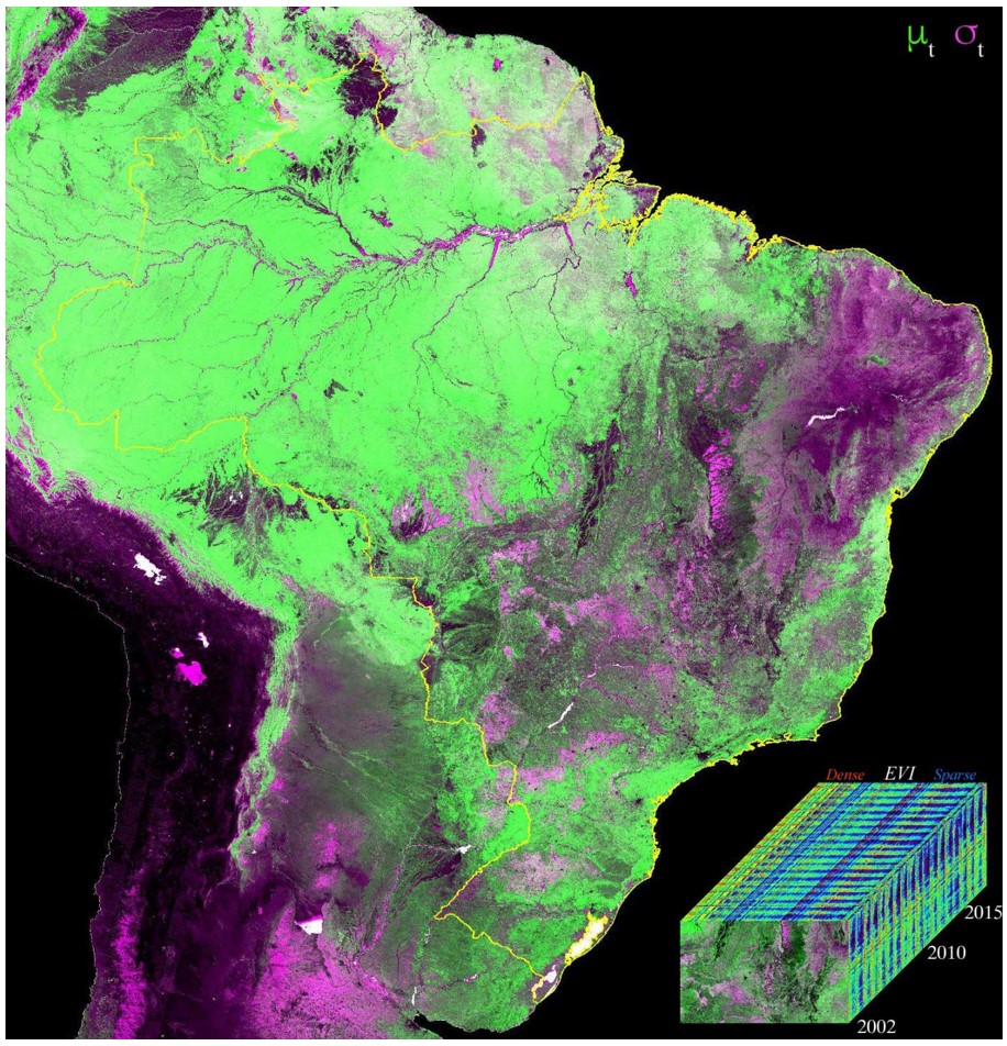
The application of the linear temporal mixture model reveals the spatiotemporal variation of vegetation phenology manifest as landscape dynamics. Figure 1 shows the spatial distribution of vegetation density and variability across Brazil, based on the statistical analysis of the temporal mean and standard deviation of EVI.

Figure 1
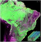
– Spatiotemporal vegetation image for study area. Temporal mean (μ_t) and standard deviation (σ_t) of MODIS Enhanced Vegetation Index (EVI) biweekly time series [2002, 2020] illustrate the continuum between evergreen (green) and seasonal (magenta) vegetation phenology. Areas with high vegetation abundance and high variability are closer to white, while sparsely vegetated areas are closer to black. Inset EVI cube illustrates the kilometer scale spatial variability of phenologic phase and amplitude among agriculture and indigenous vegetation. Source: Elaborated by the authors.

The RGB composition applied to the model enables the identification of three major landscape groupings: areas in shades of green represent homogeneous landscapes characterized by the presence of evergreen vegetation, while darker tones indicate regions with lower vegetation density and reduced temporal variability. Finally, unstable landscapes are delineated by areas in shades of magenta and white, which are marked by the presence of highly seasonal vegetation.

The EOF analysis of the MODIS EVI cube yields the variance partition shown in Figure 2. To first order, the temporal feature space is 3D, with the three low order dimensions (> 1%) accounting for 77% of total variance in the EVI cube. The next four dimensions above the noise floor account for < 1% total variance each, but correspond to deterministic (i.e. periodic) EOFs representing biannual cycles and interannual trends. EOFs of higher (> 7) dimensions lack clear periodicities and increasingly resemble noise.

Figure 2
– Variance partition for the MODIS EVI temporal feature space. To first order, the feature space is effectively 3D (> 1%), representing 77% of total variance. However, there are four additional deterministic dimensions above the continuum below the noise floor. Each of these stochastic dimensions represents < 1% of total variance, but their temporal EOFs are physically distinct, corresponding to biannual phenologies (4,5) and decadal trends (6,7). Source: Elaborated by the authors.

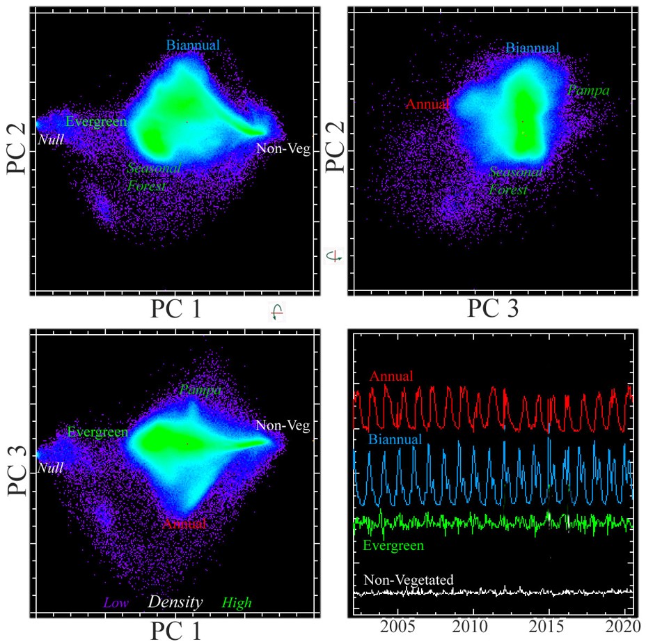
The temporal feature space spanned by the three low order EOFs is given by the space of the three low order PCs. As shown in Figure 3, orthogonal projections of the 3D PC space reveal at least four distinct apexes corresponding to temporal endmembers bounding the space. These temporal endmembers represent three distinct phenologies, as well as a fourth non-vegetated endmember with minimal variance. The endmember phenologies correspond to evergreen vegetation, an annual cycle and a biannual cycle.

Figure 3
– Temporal feature space of the low order principal components of the MODIS EVI cube. The 3D feature space has six distinct apexes corresponding to different phenologies. Temporal endmembers are shown for the four most distinct. Seasonal tropical forest is similar to evergreen but with slight seasonality. It corresponds to much of the Amazon. Pampa has strong seasonality distinct from the single cycle endmember, but corresponds only to a small area in the southwest corner of the domain. Null corresponds to locations with missing data. Unmodeled endmembers project onto the exterior of the model along mixing continua between the four modeled endmembers. Source: Elaborated by the authors.

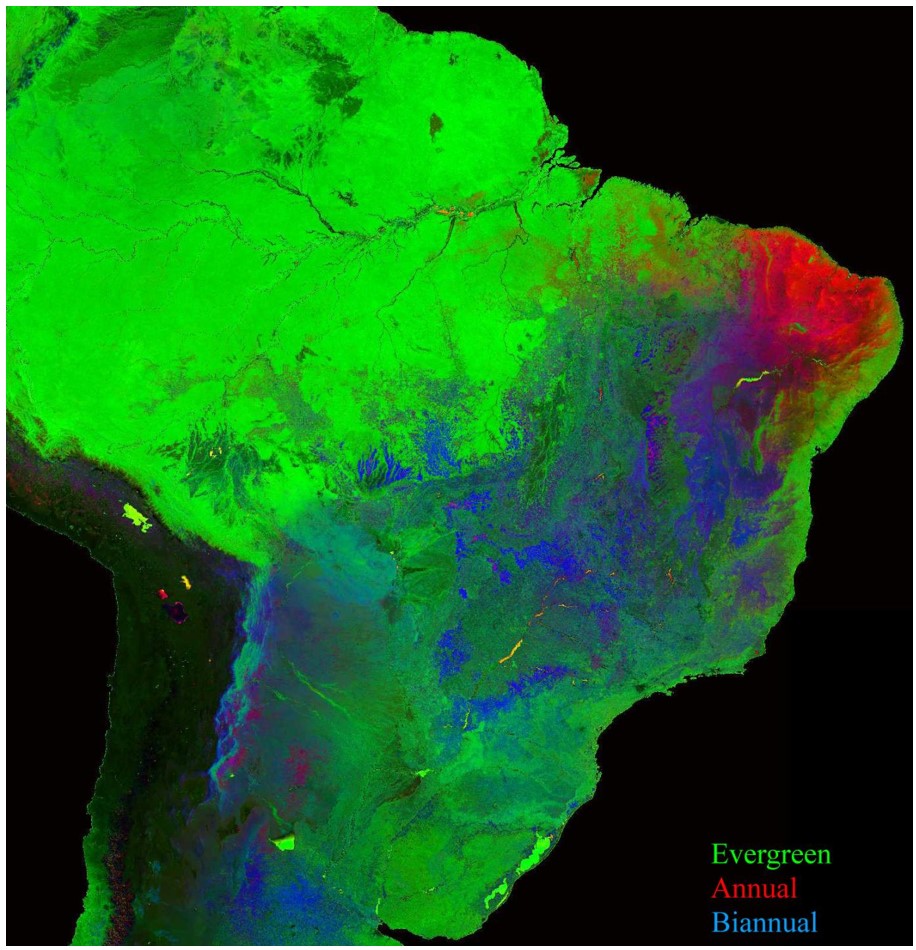
Inversion of the four endmember temporal mixture model yields a phenological fraction map for each temporal endmember (Figure 4). The fractions are generally well-bounded [0,1] with a modal RMS misfit of 0.10 (99% < 0.18). This is consistent with the variance partition showing 21% of total variance associated with the stochastic noise dimensions. This is typical for MODIS EVI in the tropics due to the relatively high frequency of cloud contamination. The fraction map in Figure 4 is broadly consistent with the climatic and biome geography of Brasil, but much more spatially detailed than any other continent-scale map to our knowledge. In addition to showing the dominant phenologies as primary colors (red, green, blue), the map shows extensive areas of phenological gradient (mixtures) as subtractive primaries (cyan, magenta, yellow). Relative vegetation abundance, modulated by the non-vegetated endmember fraction (not displayed), is manifest as the brightness and saturation of the colors on the map. Hence, less densely vegetated areas appear darker and totally unvegetated areas appear black.

Figure 4
– Vegetation phenology image derived from inversion of the four endmember temporal mixture model. Omitting the non-vegetated endmember fraction from the RGB composite renders the brightness proportional to vegetation abundance. Primary colors (RGB) correspond to the three vegetated phenologies while mixtures of primaries (e.g. cyan, magenta, yellow) correspond to intermediate or mixed phenologies. Source: Elaborated by the authors.

Because temporal EOFs 4 and 5 both represent phase-shifted binannual cycles, they provide some additional detail on the seasonal phase of the binannual endmember. Figure 5 shows these temporal EOFs and the geographic distribution of their corresponding spatial PCs. While the biannual phenology fraction corresponds to difference between EOFs 4 and 5 (black), some distinct geographies of different phase (red) are apparent. Because these two dimensions together account for only 1.1% of total variance, they are most relevant in areas with significant fractions of the biannual phenology (blue in Figure 4).

Figure 5
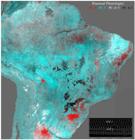
– Biannual phenology PC composite of dimensions 4 (red) and 5 (cyan). As both biannual phenologies contribute to the double crop agricultural endmember, they are implicitly represented in the 4 endmember model, but highlight the phase variability within the double crop endmember. Note that EOF pairs 2 & 3 and 4 & 5 are each phase shifted so that each pair’s PCs forms a phase plane capable of representing phase shifts in the single (2 & 3) and double (4 & 5) cycles. Source: Elaborated by the authors.

Discussion

In general, the variations identified from the spatiotemporal analysis of MODIS EVI images between 2002 and 2020 represent characteristics of the major structures of the contemporary Brazilian landscape. There are clearly two predominant types of landscapes: more stable landscapes, which are remnants of older natural processes that persist to this day in greater proportion within the conserved vegetation areas of the Amazon and Pantanal biomes; and more unstable landscapes, resulting from more recent anthropogenic changes primarily associated with agricultural and livestock production, generating the suppression and fragmentation of natural vegetation, as observed in the Cerrado, Atlantic Forest, Caatinga, and Pampa.

The analysis of vegetation density and variability (Figure 1) identified a highly synthetic representation of these two types of landscapes. Notably, there is an extensive area shaded in green in the northern region of Brazil, corresponding to the Amazon Rainforest, which exhibits higher density and lower variability in vegetation. Despite the interannual climatic variations in the Amazon region due to the El Niño-Southern Oscillation (ENSO) phenomenon (Marengo et al., 2009), the temporal mean and standard deviation of the vegetation data indicate the resilience of the tropical forest over nearly 20 years.

In the central region of Figure 1, a complexity of darker shades of green is observed, related to wet areas such as the Pantanal (Central-West in the figure) and the Araguaia Basin (Central-North in the figure). Shades of greenish gray, which exhibit greater variability, correspond to the vegetation formation of the Cerrado. The magenta tones indicate areas with lower density and high variability of vegetation. We can distinguish two groups of magenta tones: the first relates to the characteristics of vegetation formation, as seen in the Caatinga (Northeast in the figure); the second pertains to areas designated for the cultivation of crops such as soybean, corn, sugarcane, and cotton in the southern, southeastern, and central-western regions.

According to Kayano and Andreoli (2009), the climate in the Northeast region of Brazil exhibits significant interannual variability, particularly with respect to precipitation, with some years being extremely dry and others rainy. Ab’Saber (2003) emphasizes that for the daily lives of the inhabitants of the sertão and their survival, the most critical factor lies in the periodic climatic irregularities that afflict the social spaces of the dry hinterlands. This climatic variability, along with other factors such as topography and soil types, is reflected in the variation of vegetation, resulting in a distinct delineation of the boundaries of the Caatinga Domain - semi-arid intermontane and interplateau depressions,

Observing the phenology image (Figure 4), it is possible to define a landscape unit associated with phenologies that exhibit a more homogeneous rhythm of phenological variation and greater stability, representing the evergreen forested areas of Brazil. This unit is predominantly identified in the interior of the Amazon biome but is also present in parts of the Atlantic Forest biome, following the coastal facade and interior boundaries, where the Mixed Ombrophilous Forest is prominent. To the south of Brazil, this homogeneous landscape follows the contours of the Pampa biome, where the presence of grasses and shrubs, characterized by low growth, changes little over time, thereby illustrating the homogeneity and stability of this landscape pattern.

The phenology map (Figure 4) also enables the delineation of unstable landscape units (shades closer to red and purple) corresponding to the Caatinga and Cerrado biomes. These areas are characterized by phenologies where seasonality is the determining element, either due to the presence of a well-defined dry season or the advance of the agricultural frontier, particularly in the Cerrado, where annual and biannual crops occupy extensive areas. Shades of purple and blue indicate, for example, the flat-topped plateaus (chapadões) in western Bahia, as well as the cultivation areas near Chapada Diamantina. In the transition between the Cerrado and Amazon biomes, particularly in the central-northern region of Mato Grosso state, another area with biannual growth phenology is highlighted, corresponding to the main agricultural production zone of the state.

The biannual phase image (Figure 5) highlights variations in biannual phenology, thus representing areas of perennial agriculture or regions where cultivation occurs twice a year. This figure emphasizes the cultivation areas located in the pre-coastal plateaus of northeastern Brazil, the agricultural frontier of western Bahia linked to soybean cultivation in the Barreiras region, the grain crops in southern Goiás and the Triângulo Mineiro, the grain production zones of Mato Grosso and Mato Grosso do Sul, and finally, the established grain cultivation areas in western Paraná, São Paulo, and northern Rio Grande do Sul. Part of the variation can be explained by the intercalated soybean and corn harvests in some regions, as well as summer and winter crops. The variability represented by this landscape unit arises from the fact that it encompasses areas where land-use reconversion is more intense, appearing interspersed within the homogeneous/stable landscape unit or along its edges, which ultimately places pressure on this landscape unit, where the forested element remains constant over time.

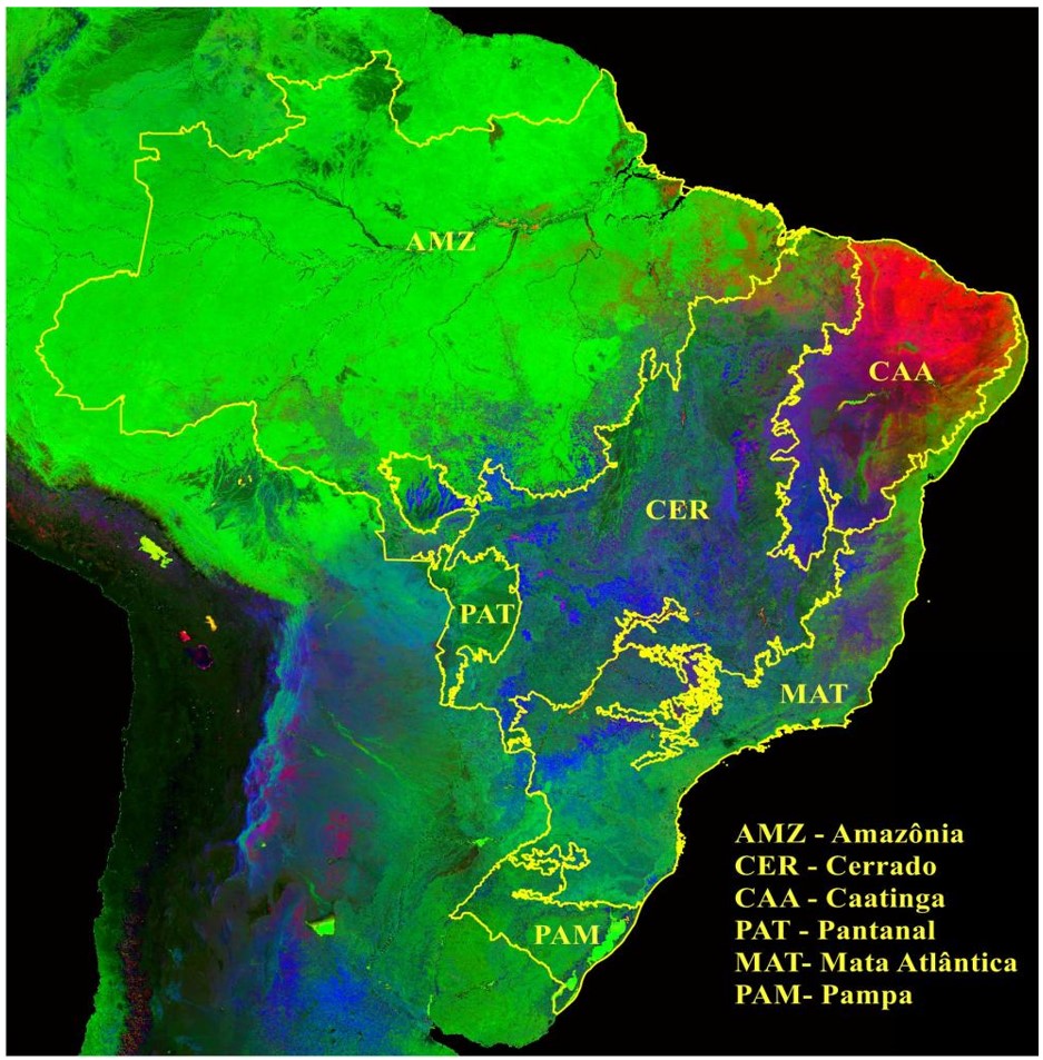
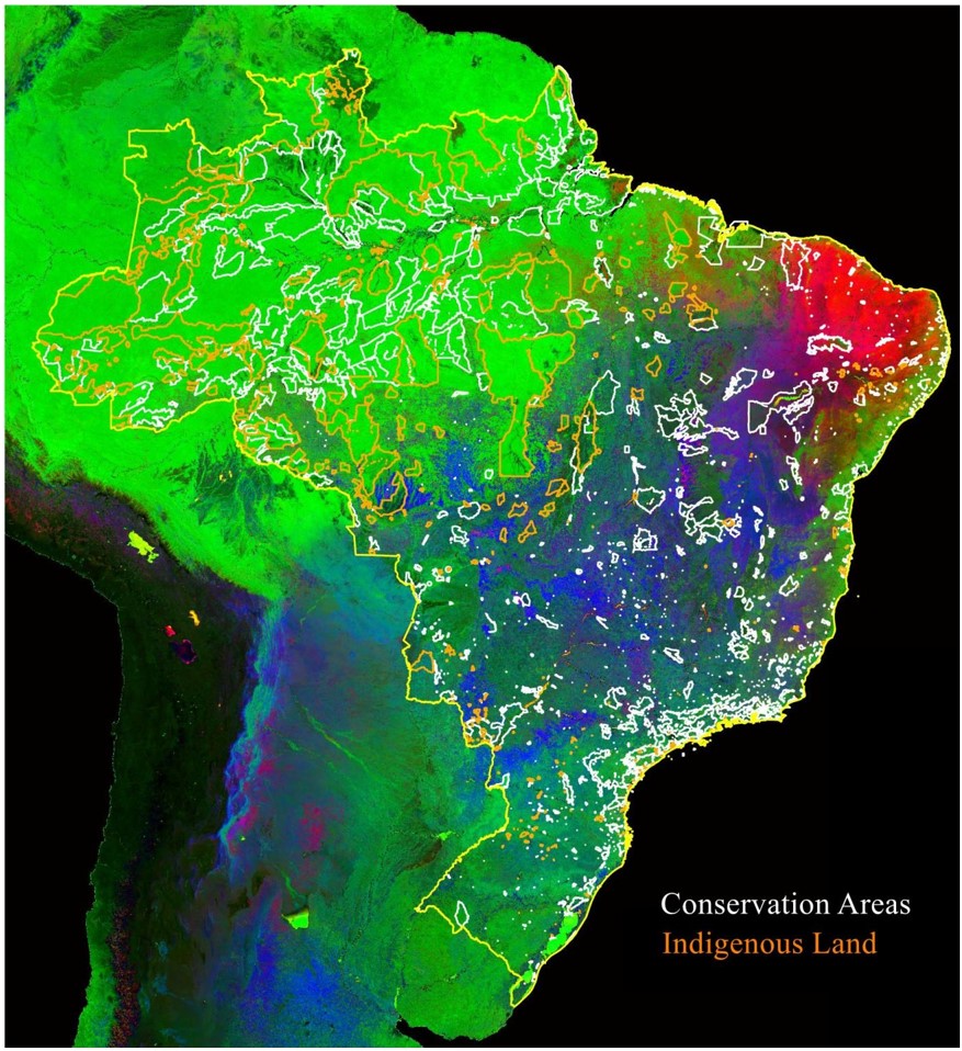
The phenology image (Figure 4) can be interpreted in the context of Brazilian biomes, Conservation Units, Indigenous Lands, and the agricultural crops of soybean, sugarcane, coffee, and rice (Figures 6, 7 and 8).

Figure 6
– Brazilian Biomes (IBGE) overlaying the phenology image. AMZ - Amazônia. CER - Cerrado, CAA - Caatinga, PAT - Pantanal., MAT - Mata Atlântica e PAM - Pampa. Source: Elaborated by the authors.

Figure 7
– Conservation Units (Integral and Sustainable Use) and Indigenous Lands within the Brazilian territory overlaying the phenology image. Source: Elaborated by the authors.

Figure 8
– Agricultural crops of soybeans, sugarcane, coffee, and rice in Brazilian territory (2019-2021) overlaying the phenology image. Source: Elaborated by the authors.

The boundaries of Brazilian biomes do not correspond with the limits of the landscape units indicated by the temporal study of phenology. For the Amazon biome, Figure 6 represents stable phenology over time, with abundant vegetation typical of evergreen areas. Darker tones indicate the absence of vegetation (water), while shades close to brown and purple refer to annual and biennial crops, confined to the Arc of Deforestation. In the Caatinga biome, phenology is depicted in shades of red, describing a pattern associated with less dense vegetation cover and marked seasonality. Purple tones, concentrated in the southern portion of the biome, indicate annual and biennial crops, while green tones represent the ecotones typical of the Caatinga-Atlantic Forest transition. In the Cerrado biome, a mix of green, purple, and red shades appears. The green tones are associated with the Cerrado-Amazon Forest and Cerrado-Atlantic Forest ecotones, whereas the red tones represent the Cerrado-Caatinga ecotones. Finally, the areas marked in purple reflect annual and biennial crops typical of the consolidated and expanding agricultural areas in Brazil. In the Pantanal biome, darker green tones predominate, characteristic of areas with persistent vegetation cover but lower density. In the Atlantic Forest biome, green tones prevail, typical of dense evergreen vegetation, alongside purple hues, characteristic of annual and biennial agriculture. Lastly, in the Pampa biome, darker green shades indicate areas of evergreen vegetation, although with lower density.

There is a spatial relationship between the distribution of Conservation Units (UCs) and Indigenous Lands (TIs) in Brazil and more stable landscapes, such as in the Amazon biome, where a large number of UCs and TIs cover extensive areas, resulting in a vast mosaic of protection for the world's largest tropical rainforest (Figure 7). This strategic arrangement ensures the maintenance of the landscape's minimal structure. However, the figure also highlights the lack of similar territorial and environmental planning for other biomes, such as the Cerrado, Caatinga, Pantanal, Atlantic Forest, and Pampa. Although a few UCs with extensive areas exist in the Cerrado, Caatinga, and Atlantic Forest, the majority are smaller, representing a low percentage of the total area under protection within these biomes and lacking structural connectivity among them.

The Atlantic Forest has a long history of landscape transformations which underwent large-scale suppression and fragmentation since the Portuguese colonization over 500 years ago. It is home to a significant portion of Brazil's population, concentrated along the Atlantic coastal zone, including major metropolitan areas such as São Paulo, Rio de Janeiro, and Curitiba (Dean, 2004). In contrast, other biomes, such as the Cerrado, Caatinga, Pantanal, and Pampa, have undergone more recent large-scale spatial transformations, underscoring the lack of conservation planning for these territories.

The relationship between agricultural cultivation areas in Brazil and temporal phenological variations (Figure 8), shows the high spatial correspondence of soybean cultivation areas with biennial phenological cycles (shown in blue tones). These cycles, analyzed in greater detail in Figure 5, are distributed from the southern edge of the Amazon, across all of the Cerrado, the southern interior of the Atlantic Forest, and the Pampa. Sugarcane crops, mainly located in the southeastern interior of the Atlantic Forest and, to a lesser extent, in the Cerrado and Pantanal, are associated with annual phenological cycles, as is rice production in southern Brazil, in the transition region between the Atlantic Forest and part of the Pampa. Coffee production is linked to more perennial cycles of vegetation variation, with its distribution concentrated in the Cerrado and the southeastern interior of the Atlantic Forest.

The results of the phenological image generally support the identifications of Brazilian landscape types made by Ross et al. (2022), distinguishing the major productive and conservation landscapes in Brazil through environmental and socioeconomic data.

Conclusion

The spatiotemporal analysis of the MODIS EVI time series reveals a significant partitioning of variance, with the first three dimensions accounting for most of the temporal variability. These dimensions outline distinct phenological patterns corresponding to evergreen vegetation, annual and biannual cycles, as well as a non-vegetated category with minimal variance.

The derived phenological fraction image demonstrates spatial patterns aligned with Brazil's climatic zones and biomes, while providing greater spatial detail compared to existing continental-scale maps. Despite the presence of stochastic noise attributed to cloud contamination, the model accurately represents the phenological diversity of the landscape, capturing both dominant and mixed phenologies with high fidelity. Additional temporal components, particularly the biannual cycles indicated by higher-order EOFs, offer further details on regional phase variations, especially in areas where biannual phenology is prominent.

The results revealed two major types of landscapes that dominate the temporal phenological variations: the first is associated with evergreen areas, primarily in the Amazon, while the second is characterized by annual and biannual cycles. It is important to highlight that while biannual cycles are more easily associated with agricultural production, annual cycles may be more challenging to distinguish between agricultural activities and natural vegetation variations, such as more open grassland areas and seasonal forest. Therefore, the spatial relationship with productive areas becomes fundamental in this type of analysis.

This applies to dense forest biomes such as the Atlantic Forest, areas with more sparse tree cover like the Cerrado and Caatinga, as well as grassland regions such as the Pampa and Cerrado. The observed phenological rhythms indicate landscapes characterized by agricultural and livestock practices, marked by greater annual and biennial variability.

The dichotomy between the vast evergreen vegetation in the Amazon and the annual and biannnual rhythms predominant in other biomes suggests a simplification of the diversity of natural rhythms. This simplification implies a loss of ecological complexity and a consequent reduction in biodiversity, as the higher annual variability patterns in managed areas contrast with the evolutionary processes occurring in forest environments. Such phenological patterns have critical implications for the conservation of biodiversity and ecological processes in Brazilian forest biomes.

The relationships observed between protected areas, such as Conservation Units associated with Indigenous Lands, and agricultural production territories underscore the importance of these strategies in maintaining spatial structures capable of supporting tropical biodiversity. However, given the current expansion of agricultural enterprises in Brazil, it has become evident that there is a need to expand the protection network at the national level for most biomes in the country.

The spatiotemporal phenological analysis demonstrates future potential for monitoring changes in landscape patterns on a national scale in Brazil. It provides insights for identifying priority regions for detailed investigation and guiding the formulation of public policies aimed at the conservation and restoration of biomes.

• How to cite this article:
  SARTOELLO, R.; ALVES FILHO, E.; SMALL, C. Exploring spatiotemporal landscape dynamics in Brazil (2002-2020): a conservation perspective. Geousp, v. 28, n. 3, e230696. 2024. https://doi.org/10.11606/issn.2179-0892.geousp.2024.230696en

References

• AB’SABER, A. N. Os domínios de natureza no Brasil: potencialidades paisagísticas. São Paulo: Ateliê Editorial, 2003.
• ANDRADE-LIMA, D.; BIGARELLA, J. J. Paleoenvironmental changes in Brazil. In: PRANCE, G. T. (ed.). Biological diversification in the tropics New York: Columbia University Press, 1982. p. 27-40.
• ARAÚJO, S. M. V. G. Origem e principais elementos da legislação de proteção à biodiversidade no Brasil. In: GANEM, R. S. (ed.). Conservação da biodiversidade, legislação e políticas públicas Brasília: Câmara dos Deputados, 2011.
• BEHLING, H. Late Quaternary vegetation, climate and fire history in the Araucaria forest and campos region from Serra Campos Gerais (Paraná), S Brazil. Review of Palaeobotany and Palynology, Amsterdam, v. 97, n. 1-2, p. 109-121, 1997. DOI: http://doi.org/10.1016/S0034-6667(96)00065-6.
  » https://doi.org/DOI: http://doi.org/10.1016/S0034-6667(96)00065-6
• BERTRAND, G. Paisagem e Geografia Física Global: esboço metodológico. Revista do Instituto de Geografia, São Paulo, v. 8, p. 141-152, 1972.
• BOARDMAN, J. W. Inversion of imaging spectrometry data using singular value decomposition. In: CANADIAN SYMPOSIUM ON REMOTE SENSING, 12., 1989, Vancouver, BC, Canada. Proceedings [...] New York: IEEE, 1989. p. 2069-2072. DOI: http://doi.org/10.1109/IGARSS.1989.577779.
  » https://doi.org/DOI: http://doi.org/10.1109/IGARSS.1989.577779
• BRASIL. Unidades de conservação Brasília: Ministério do Meio Ambiente e Mudança do Clima, 2024a. Disponível em: https://dados.gov.br/dados/conjuntos-dados/unidadesdeconservacao Acesso em: 22 out. 2024.
  » https://dados.gov.br/dados/conjuntos-dados/unidadesdeconservacao
• BRASIL. Companhia Nacional de Abastecimento. Portal de Informações Agropecuárias Brasília: CONAB, 2024b. Disponível em: https://portaldeinformacoes.conab.gov.br/mapeamentos-agricolas-downloads.html Acesso em: 22 out. 2024.
  » https://portaldeinformacoes.conab.gov.br/mapeamentos-agricolas-downloads.html
• CARNAVAL, A. C.; MORITZ, C. Historical climate modelling predicts patterns of current biodiversity in the Brazilian Atlantic Forest. Journal of Biogeography, Hoboken, v. 35, n. 7, p. 1187-1201, 2008. DOI: http://doi.org/10.1111/j.1365-2699.2007.01870.x.
  » https://doi.org/DOI: http://doi.org/10.1111/j.1365-2699.2007.01870.x
• DEAN, W. A ferro e fogo: a história e a devastação da Mata Atlântica brasileira. 1. ed. São Paulo: Cia. das Letras, 2004.
• DELPOUX, M. Ecossistema e paisagem. Métodos em Questão, São Paulo, n. 13, p. 1-23, 1974.
• FAHRIG, L. Effects of habitat fragmentation on biodiversity. Annual Review of Ecology, Evolution, and Systematics, Palo Alto, v. 34, n. 1, p. 487-515, 2003. DOI: http://doi.org/10.1146/annurev.ecolsys.34.011802.132419.
  » https://doi.org/DOI: http://doi.org/10.1146/annurev.ecolsys.34.011802.132419
• FOLEY, J. A. et al Global consequences of land use. Science, Washington, D.C., v. 309, n. 5734, p. 570-574, 2005. DOI: http://doi.org/10.1126/science.1111772. PMid:16040698.
  » https://doi.org/DOI: http://doi.org/10.1126/science.1111772
• FLENLEY, J. R. Tropical forests under the climates of the last 30,000 years. Climatic Change, London, v. 39, n. 2, p. 177-197, 1998. DOI: http://doi.org/10.1023/A:1005367822750.
  » https://doi.org/DOI: http://doi.org/10.1023/A:1005367822750
• GLOBAL FOREST WATCH. Monitoramento de Florestas Projetado para a Ação 2024. Disponível em: https://www.globalforestwatch.org Acesso em: 17 set. 2024.
  » https://www.globalforestwatch.org
• HAFFER, J. Speciation in Amazonian forest birds. Science, Washington, D.C., v. 165, n. 3889, p. 131-137, 1969. DOI: http://doi.org/10.1126/science.165.3889.131. PMid:17834730.
  » https://doi.org/DOI: http://doi.org/10.1126/science.165.3889.131
• HAWKINS, E. et al Unprecedented changes in global temperature over the past 2,000 years. Nature Climate Change, London, v. 13, n. 2, p. 131-138, 2023.
• HOORN, C. et al Amazonia through time: andean uplift, climate change, landscape evolution, and biodiversity. Science, Washington, D.C., v. 330, n. 6006, p. 927-931, 2010. DOI: http://doi.org/10.1126/science.1194585. PMid:21071659.
  » https://doi.org/DOI: http://doi.org/10.1126/science.1194585
• HUETE, A. et al Overview of the radiometric and biophysical performance of the MODIS vegetation indices. Remote Sensing of Environment, Amsterdam, v. 83, n. 1-2, p. 195-213, 2002. DOI: http://doi.org/10.1016/S0034-4257(02)00096-2.
  » https://doi.org/DOI: http://doi.org/10.1016/S0034-4257(02)00096-2
• HUETE, A.; JUSTICE, C.; VAN LEEUWEN, W. MODIS Vegetation Index (MOD13): algorithm theoretical basis document. Washington, D.C.: NASA, 1999. p. 295-309.
• INSTITUTO BRASILEIRO DE GEOGRAFIA E ESTATÍSTICA – IBGE. Pesquisa Agrícola Municipal Rio de Janeiro: IBGE, 2023. Disponível em: https://www.ibge.gov.br/ibge-digital.html Acesso em: 22 out. 2024.
  » https://www.ibge.gov.br/ibge-digital.html
• INSTITUTO BRASILEIRO DE GEOGRAFIA E ESTATÍSTICA – IBGE. Biomas Rio de Janeiro: IBGE, 2024. Disponível em: https://www.ibge.gov.br/geociencias/informacoes-ambientais/vegetacao/15842-biomas.html?=&t=downloads Acesso em: 22 out. 2024.
  » https://www.ibge.gov.br/geociencias/informacoes-ambientais/vegetacao/15842-biomas.html?=&t=downloads
• INSTITUTO INTERNACIONAL DE PESQUISA PARA O CLIMA E A SOCIEDADE – IRIDL. USGS LandDAAC MODIS version_006 2024. Disponível em: http://iridl.ldeo.columbia.edu/SOURCES/.USGS/.LandDAAC/.MODIS/.version_006/ Acesso em: 22 out. 2024.
  » http://iridl.ldeo.columbia.edu/SOURCES/.USGS/.LandDAAC/.MODIS/.version_006/
• KAYANO, M. T.; ANDREOLI, R. V. Clima da região nordeste do Brasil. In: CAVALCANTI, I. F. A. et al. (ed.). Tempo e clima no Brasil São Paulo: Oficina de Textos, 2009. v. 1, p. 213-233. Disponível em: http://urlib.net/ibi/J8LNKAN8RW/36G82NU Acesso em: 22 out. 2024.
  » http://urlib.net/ibi/J8LNKAN8RW/36G82NU
• LEDRU, M. P. et al Paleoclimate changes during the last 100,000 yr from a record in the Brazilian Atlantic rainforest region and interhemispheric comparison. Quaternary Research, Cambridge, v. 64, n. 3, p. 444-450, 2005. DOI: http://doi.org/10.1016/j.yqres.2005.08.006.
  » https://doi.org/DOI: http://doi.org/10.1016/j.yqres.2005.08.006
• LORENZ, E. N. Empirical orthogonal functions and statistical weather prediction Cambridge: MIT, 1956. (Statistical Forecasting Project, n. 48).
• MACGREGOR, G. R.; NIEUWOLT, S. Tropical climatology: an introduction to the climates of low latitudes. New York: John Wiley & Sons, 1998.
• MARENGO, J. A. et al Future change of temperature and precipitation extremes in South America as derived from the PRECIS regional climate modeling system. International Journal of Climatology, Hoboken, v. 29, n. 15, p. 2241-2255, 2009. DOI: http://doi.org/10.1002/joc.1863.
  » https://doi.org/DOI: http://doi.org/10.1002/joc.1863
• MARTIN, L. et al Mapa geológico do Quaternário Costeiro do Estado da Bahia Salvador: Secretaria de Minas e Energia, Governo do Estado da Bahia, 1980.
• MAYLE, F. E. et al Responses of Amazonian ecosystems to climatic and atmospheric carbon dioxide changes since the last glacial maximum. Philosophical Transactions of the Royal Society of London. Series B, Biological Sciences, London, v. 359, n. 1433, p. 499-514, 2004. DOI: http://doi.org/10.1098/rstb.2003.1434. PMid:15212099.
  » https://doi.org/DOI: http://doi.org/10.1098/rstb.2003.1434
• MORLEY, R. J. Origin and evolution of tropical rainforests New York: Wiley, 2000.
• ORGANIZAÇÃO DAS NAÇÕES UNIDAS PARA A ALIMENTAÇÃO E A AGRICULTURA – FAO. Fundo para o Desenvolvimento de Povos Indígenas da América Latina e Caribe – FILAC. Povos indígenas e comunidades tradicionais e a governança florestal Roma, 2021. Disponível em: https://www.fao.org/americas/priorities/indigenas-gobernanza-bosques/es Acesso em: 22 out. 2024.
  » https://www.fao.org/americas/priorities/indigenas-gobernanza-bosques/es
• PREISENDORFER, R. W. Principal component analysis in meteorology and oceanography Amsterdam: Elsevier, 1988.
• RIBAS VILAS, J. Planificación y gestión del paisaje rural. In: BOLÓS, M. (ed.). Manual de ciéncia del paisaje: teoria, método y aplicaciones. Madrid: Masson, 1992.
• ROSS, J. L. S. et al (ed.). Ordenamento territorial do Brasil: potencialidades naturais e vulnerabilidades sociais. Osasco: Ed. dos Autores, 2022. 585 p. DOI: http://doi.org/10.29327/560402.
  » https://doi.org/DOI: http://doi.org/10.29327/560402
• ROUGERIE, G.; BEROUTCHACHVILI, N. Geosystemes et paysages: Bilian et méthodes. Paris: Armand Colin, 1991. 302 p.
• SALGADO-LABOURIAU, M. L. História ecológica da Terra São Paulo: Edgard Blücher, 1994.
• SETTLE, J. J.; DRAKE, A. Linear mixing and the estimation of ground cover proportions. International Journal of Remote Sensing, London, v. 14, n. 6, p. 1159-1177, 1933. DOI: http://doi.org/10.1080/01431169308904402.
  » https://doi.org/DOI: http://doi.org/10.1080/01431169308904402
• SHEPARD, G. E. et al Miocene drainage reversal of the Amazon River driven by plate-mantle interaction. Nature Geoscience, London, v. 3, n. 12, p. 870-875, 2010. DOI: http://doi.org/10.1038/ngeo1017.
  » https://doi.org/DOI: http://doi.org/10.1038/ngeo1017
• SILVA, L. G. et al Patch size, functional isolation, visibility and matrix permeability influences Neotropical primate occurrence within highly fragmented landscapes. PLoS One, São Francisco, v. 10, n. 2, p. e0114025, 2015. DOI: http://doi.org/10.1371/journal.pone.0114025. PMid:25658108.
  » https://doi.org/DOI: http://doi.org/10.1371/journal.pone.0114025
• SMALL, C. The landsat ETM+ spectral mixing space. Remote Sensing of Environment, Amsterdam, v. 93, n. 1-2, p. 1-17, 2004. DOI: http://doi.org/10.1016/j.rse.2004.06.007.
  » https://doi.org/DOI: http://doi.org/10.1016/j.rse.2004.06.007
• SMALL, C. Spatiotemporal dimensionality and time-space characterization of multitemporal imagery. Remote Sensing of Environment, Amsterdam, v. 124, p. 793-809, 2012. DOI: http://doi.org/10.1016/j.rse.2012.05.031.
  » https://doi.org/DOI: http://doi.org/10.1016/j.rse.2012.05.031
• SMALL, C.; MILESI, C. Multi-scale standardized spectral mixture models. Remote Sensing of Environment, Amsterdam, v. 136, p. 442-454, 2013. DOI: http://doi.org/10.1016/j.rse.2013.05.024.
  » https://doi.org/DOI: http://doi.org/10.1016/j.rse.2013.05.024
• SOUSA, D.; SMALL, C. Global cross calibration of Landsat spectral mixture models. Remote Sensing of Environment, Amsterdam, v. 192, p. 139-149, 2017. DOI: http://doi.org/10.1016/j.rse.2017.01.033.
  » https://doi.org/DOI: http://doi.org/10.1016/j.rse.2017.01.033
• SOUSA, D.; SMALL, C. Which vegetation index? Benchmarking multispectral metrics to hyperspectral mixture models in diverse cropland. Remote Sensing, Basel, v. 15, n. 4, p. 971, 2023. DOI: http://doi.org/10.3390/rs15040971.
  » https://doi.org/DOI: http://doi.org/10.3390/rs15040971
• TRICART, J. Ecodinâmica Rio de Janeiro: IBGE, 1977.

Edited by

• Article editors
  Gustavo Schacht, Sueli Angelo Furlan and Karine Vargas.

Publication Dates

• Publication in this collection
  17 Mar 2025
• Date of issue
  2024

History

• Received
  22 Oct 2024
• Accepted
  14 Nov 2024