Methodology for Design and Analysis of Liquid-Cooled Heat Sinks in High-Power Density Inverters

ABSTRACT

Semiconductor switches in high-power density inverters face significant challenges related to temperature rise in their junctions, which can lead to operational failures. The design and analysis of liquid-cooled heat sinks for these inverters are complex due to their multiphysics nature, particularly under dynamic loads typical of power electronics applications. This paper presents a comprehensive methodology for the design, analysis, and evaluation of liquid-cooled heat sinks in high-power density inverters, integrating computational fluid dynamics (CFD), lumped parameter modeling, and experimental validation. The CFD method is used to determine lumped parameters, which are then incorporated into a PLECs model to simulate the thermal dynamics of semiconductor devices. Power losses calculated in PLECs are used as a reference for experimental validation, where an electronic load emulates the heat dissipation of a 30 kW traction inverter with 99% efficiency. Two liquid-cooled heat sink geometries—machined channels and a U-shaped serpentine design—are analyzed under various operational scenarios, including normal operation and failure modes in the cooling system. The results illustrate the efficacy of the proposed methodology in evaluating thermal exchange and the impact of cooling system failures on power traction inverters. This work provides a streamlined approach for designing and testing liquid-cooled heat sinks, offering valuable insights for improving thermal management in high-power density inverters.

KEYWORDS
Semiconductor technologies; High-power inverters; Liquid cooled heat sink; Computational Fluid Dynamics; Lumped parameter modeling

I. INTRODUCTION

Concerns with global warming have led government, academia, and industries to seek the development of sustainable technologies to reduce the emission of polluting gases such as CO, $C{O}_2$, $N{O}_x$ and $S{O}_x$ [¹], [²]. The pursuit of reducing the emission of polluting gases has altered the structure of the industrial production chain and the dynamics of urban mobility, particularly with the emergence of Electric Vehicles (EVs) [³]-[⁵]. According to [⁶], the transportation sector was responsible for 16% of global polluting gas emissions in 2022. In this way, the European Union (EU) and the United States of America (USA) approved legislative measures to encourage EVs. The EU has adopted changes relating to cars and vans that are in line with the targets of the Fit for 55 package, while the USA the incentive of the Reduction of Inflation Act (IRA) and Advanced Clean Cars II foresees as indicators the participation of EVs in 50% by 2030 [⁷].

The increase in investments in the electric vehicle (EV) sector necessitates advancements in electric traction inverter technologies, resulting in an enhancement of power density from 2.89 kW/L to 30.2 kW/L, as demonstrated by [⁸], [⁹]. In this context, several challenges must be addressed to improve EVs, including the development of high-performance semiconductors, batteries, power electronics technologies, and advanced thermal management system control methods for both batteries and electric traction inverters [⁹]. Specifically, semiconductor devices are crucial for electric traction inverters [¹⁰], as they handle the high power levels inherent in electric vehicles [¹¹]. Furthermore, exposing semiconductor devices to high-temperature, dusty, and humid environments limits the energy processing capabilities and lifetime of electric traction inverters [¹²]. Considering this, thermal management systems have mitigated the effects caused by over-temperature on power devices, reducing thermal stress and increasing the energy processing capability in the power system [¹³].

Improving thermal management technology for power converters is crucial to ensure that the electric drive operates within safe limits [¹⁴]-[¹⁶]. Thus, with this growing concern, thermal management systems using liquid-cooled heat sinks have been widely used to reduce thermal stress on electric traction inverters and can be accomplished through direct and double cooling techniques [¹⁷]. The growing use of these technologies in both academic and industry applications is notable. This method was applied in [¹⁸], where the authors observed that applying the technique, compared to the single-faced model, resulted in a 30-48% decrease in system thermal resistance compared with the single-sided cooling system.

Additionally, it achieved a maximum efficiency of 98.85% for a 3.3 kW buck converter [¹⁹]. The authors of [²⁰] compared different heat sink topologies, involving four models of liquid cooling heat sinks with a Serpentine Mini-Channel Heat Sink (SMCHS) type topology. The proposed evaluation consists of four heat sink configurations: Configuration A has one inlet and one outlet for the fluid; Configuration B has two serpentine channels with two inlets and two outlets in parallel longitudinally arranged; Configuration C has serpentine channels with two U-type inlets and outlets; and Configuration D has two inlets and outlets in a diagonal direction. In this study, Configuration B showed the highest heat transfer capacity among the other heat sinks, with a thermal resistance of approximately 0.16 K/W.

Paper [²¹] performed a comparative study between single and double cooling methods using Computational Fluid Dynamics (CFD) and analytical methods. The authors conducted the thermal modeling of a liquid cooling heat sink through CFD, where the thermal load originates from a 1.5 kW DC/DC converter with the presence of electrical losses. Navier-Stokes equations were used to represent the flow regime and quantify the CFD solution. Similarly, [²²] evaluated a cooling system with forced ventilation whose power ranges from 50 to 100 W per module using ANSYS Fluent software. Paper [²³], on the other hand, designed a heat sink applied to a three-phase inverter using ANSYS software, using 30 and 100 W of the power dissipated per switch and the impact of thermal conductance of the materials present and the relationship between the emergence of hot spots.

Additionally, to the previous work, the authors of [¹⁷] conducted a study on the thermal impact of driving an electric machine, considering the results obtained from CFD and PLECs software. The practical validation of thermal exchange systems presents challenges related to the instrumentation of temperature sensors, types of cooling liquids, system flow rate and data acquisition. Furthermore, the control and manipulation of the power dissipated on the thermal exchange system present inaccuracies and operational limitations. In [²⁰], a thermal validation of heat sinks is performed through a hot plate that operates with 220 V AC with 500 W which supplies heat to the heat sink. In the paper, the load power control is carried out by adjusting a continuous variable transformer. However, this approach presents challenges in managing power losses within the system due inaccuracies in controlling the heat flow across the surface of the heat sinks. In this regard, precise processes to control the amount of heat supplied to the thermal system and high-reliability data detection systems are required.

Thus, the challenges presented in the literature are limited to the accuracy and reliability of the multiplatform integration between computational simulations and practical tests, aiming at the evaluation of the heat exchange capacity under nominal conditions or in the presence of failures. This paper includes the definition of a design methodology, which covers everything from the conception of the geometry of liquid cooling systems to the obtaining of concentrated parameters, computational simulations, control of dissipated power levels and adequate instrumentation. As a result, the present paper proposes an analysis and evaluation of a liquid-cooled heat sink. This evaluation is carried out through three main steps: first, a lumped parameter modeling approach is employed using computational fluid dynamics (CFD); second, the Power Loss Estimation Calculation (PLECs) method is implemented to obtain power losses; and finally, experimental analysis is conducted using two different heat sink geometries. The lumped parameters are obtained using CFD simulations for two heat sink geometries. The first geometry consists of channel machined fins, with a cover to enclose the heat sink structure and a single input and output. The second geometry features a U-shaped serpentine design with internal channels and also employs a single input and output. Subsequently, the reference power losses are calculated using a Silicon Carbide (SiC) semiconductor, considering the lumped parameters obtained from the CFD simulations. These power losses obtained from PLECs serve as a reference for the experimental analysis. An electronic load is used to dissipate heat flux on the heat sink surfaces, emulating the power losses from a 30 kW inverter with 99% efficiency. The study then investigates junction, case, and heat sink temperatures, and operational considerations are made based on these findings. This experimental approach analyzes three different operational scenarios: the traction inverter operating without failures, operating with failures in forced ventilation of the thermal system, and the last case, operation with failure in forced ventilation and the pump electric of the thermal system. The contributions of this paper are:

• A comprehensive methodology for the experimental evaluation of heat exchange systems, encompassing the design process, computational simulations, and experimental validation, with simplified test routines tailored for rapid execution across various power inverter levels and diverse heat sink geometries;

• An evaluation of the impact of failures on thermal systems and a validation approach through simple routine tests.

II. NUMERICAL CHARACTERIZATION OF THE SYSTEM

The numerical modeling employed in this study represents the heat sink and its association with fluid dynamics in liquid-cooled heat sinks. The heat exchanges analyzed in this work are cooled by liquids flowing through internal channels, featuring a U-shaped serpentine structure and designed machined channels present in Figure 1, following the representation of the CFD approach.

FIGURE 1
Framework of the design of the heat sink geometries: (a) Design of channel machined geometry. (b) Representation of the channel machined for CFD simulations. (c) Design of U-serpentine geometry. (d) Representation of U-serpentine for CFD simulations.

A. Simulation method

The CFD simulation is developed to evaluate the thermal exchange capacity of two liquid-cooled heat sink geometries. In this approach, IGBT devices are used to generate the heat flux on the surface of the aluminum cold plate for dissipation using a liquid that flows internally. The thermal model is simulated in the ANSYS fluent package, dedicated to CFD simulations, using the Finite Volume Method [²⁴], [²⁵]. This tool was used due to the faithful characterization of the dynamics of thermal systems in fluids and solids, as it takes into account the physical and chemical properties of the materials [²⁶]. Table 1 presents the physics parameters for the heat sink models.

TABLE 1
Design parameters of the two geometries.

Parameter	U-Serpentine	Machined channels
Area (mm${}^2$)	30,000	30,000
Volume (L)	0.90	1.20
Perimeter (mm)	30x120x250	40x120x250
Diameter (mm)	19.05	19.05
Thickness (mm)	30.00	40.00
Material	Aluminium	Aluminium

B. System equation

Heat exchange systems are differentiated by their thermal exchange capacity, which comes from the internal geometry of the heat sink. This internal structure allows the fluid to transport heat away from the material, and the shape of its geometry is related to the flow regime. The flow type can be obtained through the Reynolds number, defined by equation (1),

(1) $$Re=\frac{p\cdot V\cdot D_h}{\mu }$$

where p represents the fluid density, V the flow velocity, $D_h$ the diameter, and μ the dynamic viscosity of the fluid. The flow regime can be laminar or turbulent. Reynolds numbers above 2400 characterize turbulent flow, while values below 2400 represent laminar flow [²⁷], [²⁸]. The model that describes the continuity equation is given by the differential equation (2),

(2) $$\frac{\partial u}{\partial x}+\frac{\partial v}{\partial y}+\frac{\partial w}{\partial z}=0,$$

where x, y, z are the direction vectors, and u, v, w represent the fluid velocity vectors. The energy equation for solids is given by equation (3),

(3) $$k_f\left(\frac{{\partial }^{2}T}{\partial x^2}+\frac{{\partial }^{2}T}{\partial y^2}+\frac{{\partial }^{2}T}{\partial z^2}\right)=0,$$

where $k_f$ represents the thermal conductivity of the fluid and T is the temperature.

C. Boundary conditions

The heat flow from power devices is considered unidirectional and constant, as the heat is dissipated entirely over the surface of the heat sink. Furthermore, the effect of thermal coupling is not considered in the model. The heat transfer over the heat sink is defined by:

(4) $$-k_s\frac{\partial T}{\partial y}=q\frac{\partial T}{\partial x}=\frac{\partial T}{\partial z}=0,$$

where $k_s$ is the thermal conductivity of the solid which is equivalent to 2.68 g/cm${}^3$ and q is the amount of heat. The amount of heat transferred by conduction and by convection is given, respectively, by equation (5):

(5) $$Q_{conv}=h_{av}{A}_s\left(T_{base}-T_{avf}\right),$$

where $Q_{conv}$ is the amount of heat by convection, d is the thickness of the material, $h_{av}$ is the heat transfer coefficient, $A_s$ is the surface area of the heat sink, $T_{base}$ is the base temperature of the heat sink and $T_{avf}$ is the average fluid temperature. The heat transfer between the heat sink and the external environment occurs primarily through the liquid cooling mechanism, although the ambient temperature significantly influences the process due to the heat removal from the heat sink to the coolant fluid. This process enables the determination of the average heat transfer rate, as described by Equation (6), which accounts for the system's thermophysical properties, the established thermal gradient, and the convective conditions at the solid-liquid interface. Consequently, the thermal efficiency of the assembly can be analytically determined based on predefined operational and environmental parameters,

(6) $$h_{av}=\frac{\dot{m}{C}_p\left(T_{out}-T_{in}\right)}{A_s\left(T_{base}-T_{avf}\right)},$$

where $C_p$ is the specific heat of the material, $T_{out}$ is the outlet temperature, $\dot{m}$ is the mass flow of the fluid and $T_{in}$ is the inlet temperature. Thus, the mass flow rate can be obtained by isolating it in the previous expression, resulting in

(7) $$\dot{m}=\frac{Q_{conv}}{C_p\left(T_{base}-T_{avf}\right)}.$$

The mass flow rate represents the amount of fluid mass that passes through a given area.

The geometry of the heat sink and the physical dimensions are responsible for the magnitude of the thermal resistance. The total thermal resistance of the liquid-cooled heat sink is given by

(8) $$R_{total}=\frac{T_{Dmax}-T_{Fmin}}{Q_{conv}},$$

where, $R_{total}$ is the total thermal resistance of the system, $T_{Dmax}$ is the peak temperature of the heat sink surface, and $T_{Fmin}$ is the minimum temperature due to the boundary layer of the fluid.

The implementation of the system has the following considerations: laminar flow; the gravitational force is ignored; the temperature of all parts of the system is measured on the surface; and the cooling fluid is considered incompressible.

III. THERMAL MODEL OF THE INVERTERS

The energy processing and thermal management of electric traction inverters are challenging for models with high power density. As a result, the quantification of the power dissipated by the semiconductor switches of the inverters is necessary in the design of thermal exchange systems for inverter operation within the operating limits.

A. Power losses

The power device losses during operation consist of conduction and switching losses. Conduction losses are determined by (9):

(9) $$\begin{array}{c}{P}_{con\_IGBT}=\frac{1}{T}{\displaystyle {\int }_0^t{V}_{CE}\left(t\right)I_c\left(t\right)dt}\\ P_{sw\_IGBT}=\frac{1}{T}{\displaystyle \sum _{i=1}^{T_{low}}\left[E_{on}\left(t_i\right)+E_{off}\left(t_i\right)\right]}\end{array}$$

where $P_{con\_IGBT}$ is the conduction loss in watts, $V_{CE}(t)$ is the collector-emitter voltage, $I_c(t)$ is the colletor current of the IGBT. where $P_{SW\_IGBT}$ is the switching loss in watts. $E_{on}$ is the energy dissipated during the turn-on transition, and $E_{off}$ is the energy dissipated during the turn-off transition.

B. Thermal network

The inverter thermal model represents the thermal influence of power devices, thermal interfaces and heat sinks. The thermal equivalent circuit is represented by an RC circuit, composed of resistances and capacitances that can be modeled by the Cauer and Foster thermal networks. The Cauer thermal network is represented by a second-order filter with greater precision at specific thermal frequencies in which the network parameters are thermal resistances and capacitances, while the Foster thermal network is simpler, has less precision and the network parameters are resistance and thermal constant [²⁹]. The thermal network structure used is shown in Figure 2. Where $R_{jcn}$ is the thermal resistance. $C_{jcn3}$, $C_{jcn1}$,$C_{jcn2}$ and $C_{jcn3}$ is the thermal capacitance of thermal junction. The Pout is the effective power transfer for dissipation. The $R_{hs}$ and $C_{hs}$ are the heat sink thermal resistance and capacitance. The $T_{ref}$ is the ambient temperature.

FIGURE 2
The thermal network structure of the inverter.

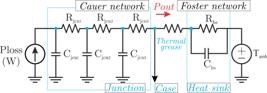
The thermal resistance of the system can be simplified using the equation (10):

(10) $$R_{jc}=\frac{\left(T_{jc}-T_{case}\right)}{P_{loss}},$$

where $R_{jc}$ is the total thermal resistance and $P_{loss}$ is the total losses of the system, given by the sum of the equations (9). Although $R_{jc}$ is commonly applied under steady-state conditions, it was used here to estimate the junction temperature. The junction temperature, using the total losses and case temperature, is obtained and difined.

(11) $$T_{jc}\left(t\right)=R_{jc}\left(t\right)P_{loss}\left(t\right)+T_{case}\left(t\right).$$

The heat flux generated by the module is determined in relation to the amount of heat transferred, taking into account the temperature variation of the surface of the heat sink, cooling liquid and the amount of heat is given by the ratio of power dissipated per area, as shown in the equation (12):

(12) $$h_f=\frac{q}{\Delta T},q=\frac{\dot{Q}}{dA}.$$

Where, the heat flux is represented by $h_f$ and the heat transfer is given by $\dot{Q}$.

IV. METHODOLOGY FOR ANALYSIS AND EVALUATION OF THE THERMAL SYSTEM

The evaluation of the thermal exchange capacity of heat sinks is conducted through the integration of CFD, PLECs simulation, and an electronic load representing the traction inverter operation. Figure 3 presents the structure of the simulation and experimental methodology. The project and design are carried out using CFD analysis, simulations of the thermal model in PLECs software, and experimental results obtained through electronic load. The steps for developing the present work are divided as follows:

FIGURE 3
Structure of the methodology for simulation and experimental results.

Step 1 - Numerical approach: Thermal parameters are obtained through the representation of a liquid-cooled heat sink using CFD simulations with ANSYS Fluent software. A heat flux is applied to the surface of the heat sink, and the RC behavior determines the thermal constant or thermal capacity. This step involves selecting the heat sink geometry and generating the mesh, which discretizes the system into several parts for individual calculation, with final results aggregated. The solution involves executing numerical methods to obtain the heat sink parameters. The algorithm utilizes CFD, problem discretization via the Finite Volume Method (FVM), and the convergence method through the system's energy balance.

Step 2 - Thermal modeling: The losses of the electric traction inverter are calculated in the PLECs software based on the parameters obtained in CFD simulation. The losses obtained serve as a reference for losses, which will be utilized for the electronic load. The inverter initially operates at 50% of the energy processing capacity and at another moment at 100% load.

Step 3 - Experimental tests: The experimental phase entails applying heat flux to the surfaces of the heat sinks through an electronic load, representing the power losses of the traction inverter. As depicted in Figure 3, the thermal system comprises a heat sink, electric pump, radiator, and heat flux generated by power IGBTs.

The first and second steps are the interchange of thermal parameters for simulating and modeling of the system, which can reduce the time needed to analyze and evaluate the thermal exchange of the liquid-cooled heat sinks. In this Figure, the first step presents the process of design through ANSYS of the cooled liquid heat sink, mesh, solution, and obtaining of thermal parameters for each geometry. For the next step, the thermal parameters are loaded in PLECs simulation to obtain the simulation results. In the last step the thermal exchange is evaluated by using the load electronic and compared with simulation results. These results can be compared and validated through the junction, case and heat sink temperature. The experimental results are necessary to validate the thermal model simulation, making it possible to reduce time analysis through tests in PLECs software.

A. Lumped parameters via CFD

Thermal networks represent a thermal exchange system incorporating thermal resistance and capacitance, enabling the determination of system temperatures. This process is streamlined using CFD, which simulates heat exchange between the heat source and the cooling fluid. The process of heating the surface of the heat sink allows for the acquisition of temperature curves for each part of the system. This procedure involves applying heat to a heat sink, where the heat originates from electrical losses due to power switching, enabling the determination of the thermal time constant of the heat sink. The thermal parameters are obtained due to the thermal behavior being analogous to a first-order resistive-capacitive (RC) electrical circuit, where the resistance represents the dissipation capacity and the thermal capacitance represents the energy storage capacity. By utilizing the relationship between temperature and the amount of energy dissipated over the heat sink, the thermal parameters are obtained, as described in [²⁰].

The thermal exchange system employs liquid cooling with an aluminum cold plate featuring internal fluid channels. Heat flux on the heat sink surface is generated by FGH60N60 IGBTs dissipating a constant amount of heat. The simulation models losses equivalent to a 30 kW inverter with 99% efficiency, operating at 50% and 100% of rated load. These losses are applied in ANSYS Fluent as heat flux ranging from 105,000 to 210,000 $W/m^2$, with an instant application at 1200 seconds and a total simulation time of 3000 seconds.

From the temperatures obtained in the CFD simulation, the thermal parameters of each heat sink are obtained using (8) and switch lumped parameters informed by the manufactures are presented in Table 2:

TABLE 2
Thermal heat sink and switch parameters.

B. Model validation in a PLECs environment

The analysis of two heat sink geometries is developed under the presence of heat flux on their surface to verify the cooling at the heat exchange level for different applied thermal loads. In this regard, the thermal parameters used consist of resistance and thermal capacitance values obtained in the CFD approach are used in this stage. The approach to the heat sink geometries involves connecting a traction inverter to an RL load with a nominal power of 30 kW. Power losses from power devices are monitored to apply thermal networks and determine system temperatures.

The temperature for each heat sink is obtained using the Foster network, while the junction temperature is calculated using the thermal Cauer network, as shown in Table 2. The simulations are conducted in two stages, considering different heat sink models. The evaluation of heat exchange systems consists of representing the losses of a 30 kW three-phase inverter through the representation of the current dynamics, applying a step from 50% to 100% of the nominal value of the inverter power. The PLECs software allows verification of system temperatures, such as switch junction temperature, case, and heat sink temperature. Figure 4 presents the junction, case, and heat sink temperatures for two geometries.

FIGURE 4
(a) Channel machined. (b) U-serpentine.

As presented, the losses resulting from the simulated inverter in the PLECs software were approximately 150 and 300 W for the operating conditions. These values were futher used as a reference for the electronic load.

C. Evaluation of the thermal exchange system

The methodology consists of verifying the heat exchange capacity for the heat sink geometries presented. The composition of the thermal exchange system is given by the heat sink receiving heat flow from an electronic board that dissipates power through power IGBTs. The structure of the electronic charge is illustrated in Figure 5. The automation of dissipated power control is managed by a control board, which handles signal generation, detection, and data storage. The power board is responsible for heat dissipation. The load electronic control is executed via an STM32F103C8T6 microcontroller, which uses a dissipated power reference to control IGBT devices. These devices generate the necessary current signal for pulse width modulation (PWM). This signal is isolated by optocouplers and filtered by a first-order filter before reaching the IGBT devices.

FIGURE 5
Structure of the control and automatizing the power losses.

The power board includes three FGH60N60 IGBTs, which are specifically chosen for their low thermal impedance connection between the junction and the case. This low thermal impedance is crucial for efficient power transfer, as it minimizes heat buildup and ensures reliable operation under high-power conditions. The evaluation system uses three power boards to accurately represent the power dissipation of a three-phase inverter operating at a 140 V bus voltage. Activation signals from the control board drive the IGBTs, ensuring smooth operation in the linear region (without switching). This approach eliminates switching losses and ensures that average conduction losses are evenly distributed across all switches. This setup provides precise control over the dissipated power through calibrated load increments, allowing for a systematic evaluation of the heat sinks cooling capabilities. Real-time temperature profiles are monitored to assess the thermal performance of the system under various operating conditions. By leveraging this configuration, the power electronic board establishes a dynamic framework for systematically validating thermal performance. This framework not only simplifies the application of heat to the heat sink surface but also ensures that the power applied is continuous and controllable, making it an ideal platform for thermal management studies.

Figure 6 presents the structure of the thermal exchange system developed, where the electronic load is shown, divided between the control and the power part that are used to control the amount of power dissipated by the IGBT switches. The composition of thermal exchange system is composed of Heat sink: Utilizes direct liquid cooling with serpentine U-shaped internal channel and fin geometries. Heat is exchanged by solid thermal conduction and solid-liquid convection, in which a ratio of 50% liquid water and 50% ethylene glycol was used. Electric pump: Drains the liquid, operating at 20 W nominal power. Heat radiator: Cools the liquid via a 30 W electric fan, with additional natural ventilation from EVs aiding in thermal exchange. Liquid tank: Supplies the radiator with replacement coolant as needed. Flow meter: Measures the velocity and area of the cooling liquid to monitor and control the flow rate.

FIGURE 6
Experimental system of the evaluation from thermal exchange systems.

V. RESULTS AND DISCUSSION

The experimental results are based on the use of an electronic load to validate the thermal exchange capacity of different models of liquid cooled heat sinks considering different operating regimes, with the representation of the operating system in different scenarios. The experimental results are based on a load step transition from 150 W to 300 W, evaluated under three distinct operating scenarios for each heat sink model. The initial conditions for carrying out the experimental tests are presented in the following Table 3, where (AT) is the ambient temperature, (FT) fluid temperature and (HsT) is the heat sink temperature and the, C represents the Channel machined and U-serpentine geomentry. The test scenarios are defined as follows:

TABLE 3
Initial temperature values for experimental evaluation.

Initial conditions (°C)		Case 1		Case 2		Case 3
		C	U	C	U	C	U
(AT)		27.20	26.70	26.20	24.80	25.40	25.40
(LT)		20.83	22.39	22.76	17.97	-	-
(HsT)		24.01	26.21	21.79	25.07	24.00	24.43

• Case 1: The heat exchange system is evaluated under normal operating conditions, with all components functioning properly. This includes the fluid flow system and the radiator's electric fan operating without any failures.

• Case 2: The system is tested with a simulated failure in the radiator's electric fan while the pressure pump continues to operate. In this scenario, the liquid flows through the heat radiator, but without the presence of forced ventilation.

• Case 3: The test involves evaluating the thermal performance under a dual-failure condition, where both the radiator's forced ventilation system and the pressure pump are non-operational. This scenario assesses the system's behavior in the absence of both forced airflow and liquid circulation.

The fluid temperature is not presented for case 3 due to the failure of the electric pump, which results in the absence of fluid flow. Consequently, thermal exchange is not effective in this situation, and the temperature profile is not presented. Thus, the results are divided between each heat sink geometry for the different operating cases. Figure 7 presents the results obtained for junction temperature, case temperature, and heat sink temperature for the channel machined geometry and U-serpentine geometry. For each result figure, the respective case is provided, with the junction, case, and heat sink temperatures presented sequentially.

FIGURE 7
Experimental results for different operations cases. (a) Channel machined geometry. (b) U-serpentine geometry.

The system showed a progressive increase in temperature for the applied power. For Case 1, the results demonstrated the thermal exchange capacity of the machined channel and U-serpentine geometries in dissipating the power loss levels applied to the electronic load. The machined channel exhibited less temperature variation compared to the U-serpentine geometry. However, both geometries achieved a steady-state behavior. In Case 2, the absence of forced ventilation resulted in slow heat exchange between the cooling fluid and the environment, reducing the electronic system's ability to operate at high power levels for extended periods. The results for Case 2 indicated a significant temperature increase for both geometries, demonstrating that failure in forced ventilation leads to high junction temperatures in the semiconductor. For Case 3, the experiment, which considered failures in both components of the system, was terminated by the electronic load power PCB protection system due to the junction temperature exceeding the 80°C limit. Consequently, the power step was not applied in this case. Complete failure in thermal management resulted in high junction temperatures for both geometries, with temperatures continuing to rise, potentially causing damage to the semiconductor.

The cooling system used in the heat sinks proved efficient only in the first case, where both an electric fan and an electric pump were operational without any failures. The absence of components in the heat exchanger system increases the thermal resistance, leading to a rise in the system's temperature. Therefore, a second and third cases are impractical due to the progressive temperature increase in all parts of the system.

VI. CONCLUSION

This work analyzed and evaluated the thermal capacity of liquid-cooled heat sinks applied in inverters, through the interaction between CFD, PLECs and experimental approaches. The analysis and evaluation were conducted through a thermal model, where the thermal parameters were obtained from CFD simulations of the two heat sink models, and the power losses for the electronic load were calculated using PLECs. Furthermore, experimental tests were conducted to evaluate the operating temperature of the thermal system under different operational conditions. The sequence of tests and steps performed is crucial for the validation of the heat sinks. These test sequences are important for determining the operational capacity in the event of failures in the thermal system in traction inverters. Additionally, it is possible to conduct thermal management tests without exposing the traction inverter intended for use in the final application.

ACKNOWLEDGMENT

This work was supported by Coordenação de Aperfeiçoamento de Pessoal de Nível Superior - Brasil (CAPES/PROEX) - Finance Code 001. The authors would also like to thank the Fundação de Desenvolvimento da Pesquisa - Fundep Mover/Linha V 27192.03.01/2022.04-00, FAPERGS TO 21/2551-002147-0 and CNPq 316714/2021-6.

• PLAGIARISM POLICY
  This article was submitted to the similarity system provided by Crossref and powered by iThenticate – Similarity Check.

REFERENCES

• ¹ N. Watts, M. Amann, N. Arnell, S. Ayeb-Karlsson, J. Beagley, K. Belesova, M. Boykoff, P. Byass, W. Cai, D. Campbell-Lendrum, et al., “The 2020 report of the Lancet Countdown on health and climate change: responding to converging crises”, The Lancet, vol. 397, no. 10269, pp. 129–170, 2021, doi: 10.1016/S0140-6736(20)32290-X.
  » https://doi.org/10.1016/S0140-6736(20)32290-X
• ² C. Pelletier, Y. Rogaume, L. Dieckhoff, G. Bardeau, M.-N. Pons, A. Dufour, “Effect of combustion technology and biogenic CO2 impact factor on global warming potential of woodto-heat chains”, Applied energy, vol. 235, pp. 1381–1388, 2019, doi: 10.1016/j.apenergy.2018.11.060.
  » https://doi.org/10.1016/j.apenergy.2018.11.060
• ³ R. Lauvergne, Y. Perez, M. Françon, A. T. De La Cruz, “Integration of electric vehicles into transmission grids: A case study on generation adequacy in Europe in 2040”, Applied Energy, vol. 326, p. 120030, 2022, doi: 10.1016/j.apenergy.2022.120030.
  » https://doi.org/10.1016/j.apenergy.2022.120030
• ⁴ L. Lander, E. Kallitsis, A. Hales, J. S. Edge, A. Korre, G. Offer, “Cost and carbon footprint reduction of electric vehicle lithium-ion batteries through efficient thermal management”, Applied Energy, vol. 289, p. 116737, 2021, doi: 10.1016/j.apenergy.2021.116737.
  » https://doi.org/10.1016/j.apenergy.2021.116737
• ⁵ F. Asgarian, S. R. Hejazi, H. Khosroshahi, “Investigating the impact of government policies to develop sustainable transportation and promote electric cars, considering fossil fuel subsidies elimination: A case of Norway”, Applied Energy, vol. 347, p. 121434, 2023, doi: 10.1016/j.apenergy.2023.121434.
  » https://doi.org/10.1016/j.apenergy.2023.121434
• ⁶ International Energy Agency, “Trends in Electric Light Duty Vehicles”, https://www.iea.org/reports/global-ev-outlook-2023/trends-inelectric-light-duty-vehicles, 2023.
  » https://www.iea.org/reports/global-ev-outlook-2023/trends-inelectric-light-duty-vehicles
• ⁷ J. Falck, C. Felgemacher, A. Rojko, M. Liserre, P. Zacharias, “Reliability of power electronic systems: An industry perspective”, IEEE Industrial Electronics Magazine, vol. 12, no. 2, pp. 24–35, 2018, doi: 10.1109/MIE.2018.2825481.
  » https://doi.org/10.1109/MIE.2018.2825481
• ⁸ R. H. Staunton, T. A. Burress, L. D. Marlino, Evaluation of 2005 Honda Accord hybrid electric drive system, Oak Ridge National Laboratory, Oak Ridge, TN, 2006, doi: 10.2172/891260.
  » https://doi.org/10.2172/891260
• ⁹ J. Reimers, L. Dorn-Gomba, C. Mak, A. Emadi, “Automotive traction inverters: Current status and future trends”, IEEE Transactions on Vehicular Technology, vol. 68, no. 4, pp. 3337–3350, 2019, doi: 10.1109/TVT.2019.2897899.
  » https://doi.org/10.1109/TVT.2019.2897899
• ¹⁰ C. Qian, A. M. Gheitaghy, J. Fan, H. Tang, B. Sun, H. Ye, G. Zhang, “Thermal management on IGBT power electronic devices and modules”, Ieee Access, vol. 6, pp. 12868–12884, 2018, doi: 10.1109/ACCESS.2018.2793300.
  » https://doi.org/10.1109/ACCESS.2018.2793300
• ¹¹ D. Reusch, J. Strydom, A. Lidow, “Thermal evaluation of chip-scale packaged gallium nitride transistors”, IEEE Journal of Emerging and Selected Topics in Power Electronics, vol. 4, no. 3, pp. 738–746, 2016, doi:JESTPE.2016.2587479.
  » https://doi.org/JESTPE.2016.2587479
• ¹² U.-M. Choi, S. Jørgensen, F. Blaabjerg, “Impact of cooling system capacity on lifetime of power module in adjustable speed drives”, IEEE Journal of Emerging and Selected Topics in Power Electronics, vol. 7, no. 3, pp. 1768–1776, 2019, doi:JESTPE.2019.2912387.
  » https://doi.org/JESTPE.2019.2912387
• ¹³ C. Zhang, S. Srdic, S. Lukic, Y. Kang, E. Choi, E. Tafti, “A SiC-based 100 kW high-power-density (34 kW/L) electric vehicle traction inverter”, in 2018 IEEE Energy Conversion Congress and Exposition (ECCE), pp. 3880–3885, IEEE, 2018, doi: 10.1109/ECCE.2018.8558373.
  » https://doi.org/10.1109/ECCE.2018.8558373
• ¹⁴ E. O. Prado, P. C. Bolsi, H. C. Sartori, J. R. Pinheiro, “Modelo analítico de cálculo de perdas em MOSFETs de potência para aplicação em banco de dados”, Eletrônica de Potência, vol. 26, no. 4, pp. 388–398, 2021, doi: 10.18618/REP.2021.4.0023.
  » https://doi.org/10.18618/REP.2021.4.0023
• ¹⁵ A. Lajunen, Y. Yang, A. Emadi, “Recent developments in thermal management of electrified powertrains”, IEEE Transactions on Vehicular Technology, vol. 67, no. 12, pp. 11486–11499, 2018, doi: 10.1109/TVT.2018.2876315.
  » https://doi.org/10.1109/TVT.2018.2876315
• ¹⁶ D. Kong, R. Peng, P. Ping, J. Du, G. Chen, J. Wen, “A novel battery thermal management system coupling with PCM and optimized controllable liquid cooling for different ambient temperatures”, Energy conversion and management, vol. 204, p. 112280, 2020, doi: 10.1016/j.enconman.2019.112280.
  » https://doi.org/10.1016/j.enconman.2019.112280
• ¹⁷ G. Mademlis, R. Orbay, Y. Liu, N. Sharma, R. Arvidsson, T. Thiringer, “Multidisciplinary cooling design tool for electric vehicle SiC inverters utilizing transient 3D-CFD computations”, eTransportation, vol. 7, p. 100092, 2021, doi: 10.1016/j.etran.2020.100092.
  » https://doi.org/10.1016/j.etran.2020.100092
• ¹⁸ B. Li, X. Yang, K. Wang, H. Zhu, L. Wang, W. Chen, “A compact double-sided cooling 650v/30a gan power module with low parasitic parameters”, IEEE Transactions on Power Electronics, vol. 37, no. 1, pp. 426–439, 2021, doi: 10.1109/TPEL.2021.3092367.
  » https://doi.org/10.1109/TPEL.2021.3092367
• ¹⁹ D. Reusch, J. Strydom, A. Lidow, “Thermal evaluation of chip-scale packaged gallium nitride transistors”, IEEE Journal of Emerging and Selected Topics in Power Electronics, vol. 4, no. 3, pp. 738–746, 2016, doi:JESTPE.2016.2587479.
  » https://doi.org/JESTPE.2016.2587479
• ²⁰ A. A. Imran, N. S. Mahmoud, H. M. Jaffal, “Numerical and experimental investigation of heat transfer in liquid cooling serpentine mini-channel heat sink with different new configuration models”, Thermal Science and Engineering Progress, vol. 6, pp. 128–139, 2018, doi: 10.1016/j.tsep.2018.03.011.
  » https://doi.org/10.1016/j.tsep.2018.03.011
• ²¹ A. P. Catalano, C. Scognamillo, V. d’Alessandro, A. Castellazzi, “Numerical simulation and analytical modeling of the thermal behavior of singleand double-sided cooled power modules”, IEEE Transactions on Components, Packaging and Manufacturing Technology, vol. 10, no. 9, pp. 1446–1453, 2020, doi: 10.1109/TCPMT.2020.3007146.
  » https://doi.org/10.1109/TCPMT.2020.3007146
• ²² C. Bünnagel, S. Monir, A. Sharp, A. Anuchin, O. Durieux, Uria, Y. Vagapov, “Forced air cooled heat sink with uniformly distributed temperature of power electronic modules”, Applied Thermal Engineering, vol. 199, p. 117560, 2021, doi: 10.1016/j.applthermaleng.2021.117560.
  » https://doi.org/10.1016/j.applthermaleng.2021.117560
• ²³ J. Ye, K. Yang, H. Ye, A. Emadi, “A Fast Electro-Thermal Model of Traction Inverters for Electrified Vehicles”, IEEE Transactions on Power Electronics, vol. 32, no. 5, pp. 3920–3934, 2017, doi: 10.1109/TPEL.2016.2585526.
  » https://doi.org/10.1109/TPEL.2016.2585526
• ²⁴ M. Yang, M. Moghimi, R. Loillier, C. Markides, M. Kadivar, “Design of a latent heat thermal energy storage system under simultaneous charging and discharging for solar domestic hot water applications”, Applied Energy, vol. 336, p. 120848, 2023, doi: 10.1016/j.apenergy.2023.120848.
  » https://doi.org/10.1016/j.apenergy.2023.120848
• ²⁵ X. Hu, H. Takazawa, K. Nagase, M. Ohta, A. Yamamoto, “Threedimensional finite-element simulation for a thermoelectric generator module”, Journal of Electronic Materials, vol. 44, pp. 3637–3645, 2015, doi: 10.1007/s11664-015-3898-y.
  » https://doi.org/10.1007/s11664-015-3898-y
• ²⁶ D. Luo, Y. Yan, Y. Li, R. Wang, S. Cheng, X. Yang, D. Ji, “A hybrid transient CFD-thermoelectric numerical model for automobile thermoelectric generator systems”, Applied Energy, vol. 332, p. 120502, 2023, doi: 10.1016/j.apenergy.2022.120502.
  » https://doi.org/10.1016/j.apenergy.2022.120502
• ²⁷ B. A. Simon, A. Gayon-Lombardo, C. A. Pino-Muñoz, C. E. Wood, K. M. Tenny, K. V. Greco, S. J. Cooper, A. Forner-Cuenca, F. R. Brushett, A. R. Kucernak, et al., “Combining electrochemical and imaging analyses to understand the effect of electrode microstructure and electrolyte properties on redox flow batteries”, Applied Energy, vol. 306, p. 117678, 2022, doi: 10.1016/j.apenergy.2021.117678.
  » https://doi.org/10.1016/j.apenergy.2021.117678
• ²⁸ P. Liu, J. Li, H. Su, D. Sun, M. Yu, X. Yuan, “Wall temperature effects on wall heat flux in high-enthalpy turbulent boundary layers”, Aerospace Science and Technology, p. 108432, 2023, doi: 10.1016/j.ast.2023.108432.
  » https://doi.org/10.1016/j.ast.2023.108432
• ²⁹ M. Xu, K. Ma, B. Liu, X. Cai, “Modeling and correlation of two thermal paths in frequency-domain thermal impedance model of power module”, IEEE Journal of Emerging and Selected Topics in Power Electronics, vol. 9, no. 4, pp. 3971–3981, 2020, doi: 10.1109/JESTPE.2020.3034574.
  » https://doi.org/10.1109/JESTPE.2020.3034574

Edited by

• Associate Editor
  Allan F. Cupertino https://orcid.org/0000-0001-8418-1985

• Editor-in-Chief
  Heverton A. Pereira https://orcid.org/0000-0003-0710-7815

Publication Dates

• Publication in this collection
  11 Aug 2025
• Date of issue
  2025

History

• Received
  08 Jan 2025
• Accepted
  30 Apr 2025
• Published
  12 May 2025