Bayesian modeling of herbicide dose-response curves with maximum entropy priors

Modelagem bayesiana da curva de dose-resposta de herbicidas com priori de máxima entropia

ABSTRACT:

Several factors influence the agricultural sector, and weed interference is one of the most damaging factors in crop development and productivity. One of the most common strategies for controlling weeds is the use of herbicides, the efficiency of which is evaluated by the relationship between the dose and response in plants and can be described by nonlinear regression models. This study used Bayesian inference with maximum entropy priors for the parameters of the nonlinear, logistic, and Weibull models to describe the dose-response data of five Amaranthus weed species subjected to the herbicide trifloxysulfuron-sodium. The doses tested were 16D, 4D, D, 1/4D, 1/16D, 1/64D, and 0, where D is the recommended dose of 3.75 g ha^-1 in the first application, and 7.5 g ha^-1 in the second. The results indicated that the Groot model best described the data for A. deflexus, A. spinosus, and A. retroflexus, while the logistic model was more appropriate for A. viridis and A. hybridus. No significant differences were detected between the maximum and minimum controls; however, the doses required to achieve a 50% control varied. These values were lower for A. retroflexus (0.1980 g ha^-1) and higher for A. deflexus (1.0440 g ha^-1), indicating differences in the susceptibility of these species to trifloxysulfuron-sodium.

Key words:
Bayesian inference; nonlinear models; MCMC; trifloxysulfuron-sodium; susceptibility

RESUMO:

O setor agropecuário é influenciado por diversos fatores, sendo a interferência de plantas daninhas um dos que mais comprometem o desenvolvimento e a produtividade das culturas. Dentre as estratégias adotadas para seu controle, destaca-se o uso de herbicidas, cuja eficiência é avaliada por meio da relação entre a dose e a resposta nas plantas, podendo ser descrita por modelos de regressão não linear. Este trabalho teve como objetivo aplicar a inferência bayesiana, utilizando a priori de máxima entropia nos parâmetros dos modelos não lineares de Groot, logístico e Weibull, para descrever os dados de dose-resposta de cinco espécies de plantas daninhas do gênero Amaranthus, submetidas ao herbicida trifloxysulfuron-sodium. Foram utilizadas doses de 16D, 4D, D, 1/4D, 1/16D, 1/64D e ausência, sendo D a dose recomendada do produto, aplicada em duas conduções: 3,75 g ha^-1 na primeira e 7,5 g ha^-1na segunda. Os resultados indicaram que o modelo de Groot melhor descreveu os dados para as espécies A. deflexus, A. spinosus e A. retroflexus, enquanto o modelo logístico foi mais adequado para A. viridis e A. hybridus. Embora não tenham sido observadas diferenças significativas entre os controles máximos e mínimos, as doses necessárias para atingir 50% de controle variaram, sendo menores para A. retroflexus (0,1980 g ha^-1) e maiores para A. deflexus (1,0440 g ha^-1), evidenciando diferenças na suscetibilidade dessas espécies ao herbicida.

Palavras-chave:
inferência bayesiana; modelos não lineares; MCMC; trifloxysulfuron-sodium; suscetibilidade.

INTRODUCTION

There are several species of weeds known worldwide. Among them, the Amaranthus genus stands out. This genus belongs to the family Amaranthaceae and is widely distributed in Brazil. These plants compete directly with crops for environmental resources such as water, light, nutrients, carbon dioxide, and space. This competition can reduce crop production and quality, causing economic losses for farmers (MOROTA et al., 2020; KESHTKAR et al., 2021).

Several techniques are used to control weeds, including preventive management and cultural, mechanical, physical, biological, and chemical control methods. One of the most widely used techniques is chemical control, which involves using synthetic chemical products called herbicides. In adequate doses, herbicides can kill or slow the growth of plants (MOROTA et al., 2020).

Trifloxysulfuron-sodium is a selective post-emergent herbicide that inhibits Acetolactate Synthase (ALS), an enzyme essential for weed growth. This results in the weeds’ death. It is generally used for cotton and sugarcane crops. Trifloxysulfuron-sodium has been used to control A. retroflexus (FRANCISCHINI et al., 2019), to study the tolerance of Pima and Upland cotton species (ZHANG et al., 2021), and to control volunteer soybean (TAKAHASHI et al., 2020). In sugarcane, trifloxysulfuron-sodium was evaluated for controlling Cyperus rotundus (OLIVEIRA et al., 2010) and for its effects on the physiological characteristics of sugarcane cultivars (TORRES et al., 2012).

In South America, cases of resistance to ALS-inhibiting herbicides have been documented in species including A. hybridus, A. viridis, and A. palmeri. These herbicides account for 25% of resistance cases in Amaranthus species worldwide (YANNICCARI et al., 2023). This resistance complicates the control of these weeds and underscores the importance of investigating differences in susceptibility to herbicides, typically achieved through dose-response studies.

The relationship between dose and response can be described by nonlinear regression models, which have the advantage of allowing biological interpretation of the parameters. This approach can facilitate comprehension of the impact of herbicides on plants, promote the judicious use of chemicals, and assist in predicting the consequences of these practices on the weed population. Furthermore, it can contribute to minimizing the overall cost of production and environmental impacts (BRITO et al., 2018; FRANCISCHINI et al., 2019; KESHTKAR et al., 2021).

The Groot, logistic, and Weibull models are suitable for describing this relationship. These models are used to describe data that follow a sigmoidal (S-shaped) pattern, which increases or decreases monotonically as the dose increases (RITZ, 2010; YANG et al., 2021; KESHTKAR et al., 2021).

These models have been applied to studies of dry mass accumulation in eucalyptus and pine exposed to glyphosate (SILVA et al., 2015), in gas production in ruminant feed (MJOUN, 2018), in cross-and multiple resistance of A. retroflexus biotypes to herbicides (FRANCISCHINI et al., 2019), and cell cultures with two cancer treatments (HOLLAND-LETZ et al., 2020), in applications of herbicides such as glyphosate and bentazone, in white mustard (YANG et al., 2021), in the kinetics of in vitro gas production of corn silage (ZORNITTA et al., 2021), in the analysis of dichotomous data (SHAO et al., 2022), and in the evaluation of the susceptibility of Amaranthus species to the herbicide trifloxysulfuron-sodium (AZARIAS et al., 2024b).

The least squares method (LSM) has been used to fit nonlinear models (SARI et al., 2018; SILVA et al., 2019; JANE et al., 2020; FRUHAUF et al., 2022; AZARIAS et al., 2023; AZARIAS et al., 2024a). However, the LSM is based on an asymptotic theory and requires large samples for the estimated parameter values to approach the real values (DRAPER & SMITH, 1998; MA et al., 2020; SILVA et al., 2022). This rarely occurs in dose-response studies, which typically use small samples (MA et al., 2020).

An alternative to the least squares method (LSM) is Bayesian inference, which is based on Bayes’ theorem and treats model parameters as random variables with probability distributions. This approach is especially useful when sample data is limited (SILVA et al., 2022; FERNANDES et al., 2022). It allows researchers to incorporate their prior knowledge about the model parameters, represented by their density prior, before observing the data. According to Bayes’ theorem, combining the prior P(θ) with the data likelihood L(θ│Y) results in a posterior distribution P(θ│Y) (WANG et al., 2018; SCHOOT et al., 2021; KAPLAN, 2023).

Several methods for obtaining priors are presented in the literature (TURKMAN et al., 2019; LAMBERT, 2018; KAPLAN, 2023). However, due to the subjectivity involved in selecting priors, different approaches can lead to different results for the same problem. The maximum entropy principle is a more conservative approach that seeks to maximize uncertainty and produce less biased estimates of the phenomenon under study (JAYNES, 1957; JAYNES, 2003; CUNHA et al., 2017; BLOETSCHER et al., 2020; SILVA et al., 2022).

Several researchers have used the frequentist methodology to fit nonlinear models to data addressing dose-response relationships (BRITO et al., 2018; FRANCISCHINI et al., 2019; CANEDO et al., 2019; TESSARO et al., 2020; FRAGA et al., 2020; HASANZADEH et al., 2021; AZARIAS et al., 2024b). However, few studies in the literature use Bayesian inference to examine the dose-response relationship of herbicides in weeds.

The present study a applied Bayesian inference with maximum entropy priors to the parameters of nonlinear Groot, Weibull, and logistic models to describe the dose-response data of Amaranthus weeds to the herbicide trifloxysulfuron-sodium. The study also assessed the susceptibility of plants to the herbicide and determined the most suitable model to describe the data.

MATERIALS AND METHODS

The data used were extracted from CARVALHO et al. (2006). The experiment was conducted in a greenhouse at the Department of Plant Production of the Luiz de Queiroz College of Agriculture (ESALQ, Universidade de São Paulo), located in Piracicaba, State of São Paulo, from September to December 2005.

Seeds of A. hybridus (smooth pigweed), A. retroflexus (redroot pigweed), A. viridis (slender amaranth), A. deflexus (low amaranth), and A. spinosus (spiny amaranth) were used. The herbicide doses used were: 16D, 4D, D, 1/4D, 1/16D, 1/64D, and 0. D indicates the product’s indicated dose, which was applied in two repetitions of the experiment: 3.75 g in the first and 7.5 g ha^-1 in the second.

The experimental design was randomized blocks, with four repetitions. The experimental plots consisted of plastic pots filled with a commercial substrate, and added with 2 g of the 10:10:10 fertilizer (N: P ₂ O ₅: K ₂ O). The seeds were superficially distributed in the plots and covered with a thin layer of substrate (≈ 2 mm). Thinning was subsequently performed to maintain an average of ten plants per pot.

Post-emergence spraying was performed in a closed application chamber. The equipment used was a sprayer with flat-fan nozzles (Teejet 80.02E), with the jet positioned 0.50 m above the target surface, providing a spray volume of 200 L ha^-1. Adjuvant was used when necessary. The level of control was assessed 20 days after application (DAA), based on extreme values, where 0 indicates no control and 100% indicates plant death.

The following non-linear models were used to describe the dose-response curve data for the herbicide trifloxysulfuron-sodium:

(i) GROOT et al. (1996) model:

$y_i=\frac{a}{\left(1+\frac{b^c}{{x_i}^c}\right)}+{\mathrm{\epsilon }}_i.$

(ii) Logistic model proposed by Streibig (1988):

$y_i=\frac{a}{\left(1+{\left(\frac{x_i}{b}\right)}^c\right)}+{\mathrm{\epsilon }}_i.$

(iii) Weibull model (SEBER & WILD, 1989):

y_i = a + (d - a) exp (1 - exp (c (log (x _i ) - log (b)))) + ɛ_i

Where, i = 1, 2,...,n; y _i is the ith observation of the dependent variable, corresponding to the percentage of control; x _i is the ith observation of the independent variable, representing the herbicide doses; and a, b, c, and d, are the model parameters: a is the horizontal asymptote, a mathematical estimate of the amplitude, i.e., the maximum control minus the minimum control; b, in the Groot and logistic models, is the herbicide dose that provides 50% control; in the Weibull model, b corresponds to 63% control; in the logistic and Weibull models, c is the slope of the curve around b and in the Groot model, it is an integration constant that determines the sharpness of the curve; in the Weibull model, d represents the response of the untreated control (y at x = 0); ɛ_i are the random errors, with a normal distribution with a zero mean and variance of σ², that is, ɛ_i ~ N (0, σ²).

The Weibull, logistic, and Groot models were selected due to their widespread use in the literature and their ability to accurately describe the behavior of dose-response data. Additionally, the Groot model has a similar parameterization to the logistic model and is applied in kinetic studies. These models have already been adopted for research on dry mass accumulation in plants exposed to glyphosate (SILVA et al., 2015), A. retroflexus resistance to herbicides (FRANCISCHINI et al., 2019), white mustard control (YANG et al., 2021), in vitro gas production (ZORNITTA et al., 2021), in dichotomous data (SHAO et al., 2022), and susceptibility of Amaranthus species to herbicides (AZARIAS et al., 2024b).

The most common approaches to define distribution priors are conjugate priors, chosen for their analytical simplicity, and Jeffreys priors, which are derived from Fisher’s information (TURKMAN et al., 2019; LAMBERT, 2018). This study adopted an approach based on the maximum entropy principle, which differs in that it maximizes the uncertainty of the parameter by considering only the known moments of the distribution prior (JAYNES, 1957; JAYNES, 2003).

SHANNON (1948) established some postulates for measuring uncertainty H(X), leading to the formula for information entropy $H\left(p_1,p_2,\dots ,p_k\right)=-K{\sum }_{i=1}^k{p}_i\log p_i$, where K is a positive constant. The quantity H(X) is called the information entropy of a random variable X and refers to the thermodynamic definition of entropy and is bounded between 0 and log(k). These values represent the absence and maximum uncertainty about the events of X, respectively.

When the information about the probabilities (p _i ) is limited, the maximum entropy principle proposes choosing the distribution that maximizes entropy, while considering only the restrictions known from the data (CUNHA et al., 2017). This maximization is achieved using the Lagrange multiplier method and results in the general form $p_i=\exp \left(-{\mathrm{\lambda }}_0-{\sum }_{j=1}^m{\mathrm{\lambda }}_j{q}_{ji}\right)$, where λ₀ and λ_j are defined according to the restrictions imposed by the available information.

For continuous variables, the entropy is $h\left(X\right)=-{\int }_{-\mathrm{\infty }}^{+\mathrm{\infty }}f\left(x\right)\log f\left(x\right)dx$ where f(x) is the probability density function. Maximizing differential entropy seeks to determine probability distributions that satisfy constraints: I. (f(x) ≥ 0), $II.({\int }_{-\mathrm{\infty }}^{+\mathrm{\infty }}f\left(x\right)dx=1)$ and $III.{\int }_{-\mathrm{\infty }}^{+\mathrm{\infty }}f\left(x\right)g_i\left(x\right)dx={\mathrm{\alpha }}_i$, for i = 1,2,…,m, where g _i (x) is a function of x. Constraints I and II express two fundamental properties of probability density functions. Constraint III establishes the moments of x and summarizes the prior knowledge available about the random variable x.

Based on the principle of maximum entropy, the distribution priors were defined from the known statistical moments. We also considered the interpretation of the model parameters and information extracted from the literature on the dose-response curves for the herbicide trifloxysulfuron-sodium. The hyperparameters were defined based on the mean values reported in dose-response studies with herbicides presented in the literature (FRANCISCHINI et al., 2013; FRANCISCHINI et al., 2014; FRANCISCHINI et al., 2019; NETTO et al., 2016).

The parameter a represents the horizontal asymptote in the three models. The parameter b indicates the dose responsible for 50% of the herbicide response in the Groot and logistic models and 63% in the Weibull model. The parameter d represents the response of the untreated control. All parameters must be positive. Given that the known mean values and variance of these parameters are known, the maximum entropy distribution chosen was the truncated normal, according to equations (1), (2), and (3).

$P\left(a|{\mathrm{\mu }}_a,{\mathrm{\sigma }}_a^2\right)\propto \exp \left\{-\frac{1}{2{\mathrm{\sigma }}_a^2}{\left(a-{\mathrm{\mu }}_a\right)}^2\right\},a\in \left(0,\mathrm{\infty }\right)$ (1)

$P\left(b|{\mathrm{\mu }}_b,{\mathrm{\sigma }}_b^2\right)\propto \exp \left\{-\frac{1}{2{\mathrm{\sigma }}_b^2}{\left(b-{\mathrm{\mu }}_b\right)}^2\right\},b\in \left(0,\mathrm{\infty }\right)$ (2)

$P\left(d|{\mu }_d,{\sigma }_d^2\right)\propto \exp \left\{-\frac{1}{2{\sigma }_d^2}{\left(d-{\mu }_d\right)}^2\right\},d\in \left(0,\mathrm{\infty }\right)$(3)

As for the parameter c, which is related to the slope of the curve in the three models and, as found in the literature, can assume negative and positive values according to the literature, the chosen maximum entropy distribution was normal, since the mean values and variance of this parameter are known according to equation (4).

$P\left(c|{\mathrm{\mu }}_c,{\mathrm{\sigma }}_c^2\right)\propto \exp \left\{-\frac{1}{2{\mathrm{\sigma }}_c^2}{\left(c-{\mathrm{\mu }}_c\right)}^2\right\},c\in \left(-\mathrm{\infty },\mathrm{\infty }\right)$(4)

Since the precision, $\mathrm{\tau }=\frac{1}{{\sigma }^2}$, can only assume positive values and has a known mean value (obtained in the three models), the maximum entropy distribution considered was the exponential distribution (5).

$P\left(\mathrm{\tau }|\mathrm{\delta }\right)\propto \exp \left\{-\frac{\mathrm{\tau }}{\mathrm{\delta }}\right\},\mathrm{\tau }\in \left(0,\mathrm{\infty }\right)$(5)

Assuming ɛ_i ~ N(0, σ²), the likelihood for the Groot model can be represented as follows:

And written as a matrix:

$\propto {\mathrm{\tau }}^{\frac{n}{2}}\exp \left\{-\frac{\mathrm{\tau }}{2}{\left(\mathit{y}-\frac{a}{1+{\left(\frac{b}{\mathit{x}}\right)}^c}\right)}^{\text{'}}\left(\mathit{y}-\frac{a}{1+{\left(\frac{b}{\mathit{x}}\right)}^c}\right)\right\}$(6)

where y = (y ₁, y ₂,…,y _n )´and x = (x ₁, x ₂,…,x _n )´

Similar to the Groot model and assuming that ɛ_i ~ N(0, σ²), the likelihood for the logistic model can be represented as a matrix:

$L\left(\mathit{y}|b,a,c,\mathrm{\tau }\right)\propto {\mathrm{\tau }}^{\frac{n}{2}}\exp \left\{-\frac{\mathrm{\tau }}{2}{\left(\mathit{y}-\frac{a}{1+{\left(\frac{\mathit{x}}{b}\right)}^c}\right)}^{\text{'}}\left(\mathit{y}-\frac{a}{1+{\left(\frac{\mathit{x}}{b}\right)}^c}\right)\right\}$ (7)

where y = (y ₁, y ₂,…,y _n )´and x = (x ₁, x ₂,…,x _n )´

For the Weibull model, it can be represented as follows:

${\tau }^{n/2}exp\left\{-\frac{\mathrm{\tau }}{2}{\left[\mathit{y}-\left(a+\left(d-a\right)\exp \left\{1-exp\left\{c\left(log\left(\mathit{x}\right)-log\left(b\right)\right)\right\}\right\}\right)\right]}^{\text{'}}\times \left[\mathit{y}-\left(a+\left(d-a\right)exp\left\{1-exp\left\{c\left(log\left(\mathit{x}\right)-log\left(b\right)\right)\right\}\right\}\right)\right]\right\}$ (8)

where y = (y ₁, y ₂,…,y _n )´and x = (x ₁, x ₂,…,x _n )´.

Based on the distribution priors and the likelihood, and applying Bayes’s theorem with the parameters a, b, c, d, and τ considered independent, the joint posterior distribution of the Groot and logistic models is expressed as follows:

$P\left(a,b,c,\tau |y\right)\propto L\left(\mathit{y}|a,b,c,\tau \right)$

$P\left(a|{\mu }_a,{\sigma }_a^2\right)P\left(b|{\mu }_b,{\sigma }_b^2\right)P\left(c|{\mu }_c,{\sigma }_c^2\right)P\left(\tau |\delta \right)$

By substituting the distribution priors (1), (2), and (4), as well as the likelihood (6), and applying Bayes’ theorem, we can obtain the joint posterior for the Groot model:

$P\left(a,b,c,\mathrm{\tau }∣y\right)\propto {\mathrm{\tau }}^{\frac{n}{2}}\exp \left\{-\frac{\mathrm{\tau }}{2}{\left(\mathit{y}-\frac{a}{1+{\left(\frac{b}{\mathit{x}}\right)}^c}\right)}^{\text{'}}\left(\mathit{y}-\frac{a}{1+{\left(\frac{b}{\mathit{x}}\right)}^c}\right)\right\}$

$\times \exp \left\{-\frac{1}{2{\mathrm{\sigma }}_a^2}{\left(a-{\mathrm{\mu }}_a\right)}^2\right\}\times \exp \left\{-\frac{1}{2{\mathrm{\sigma }}_b^2}{\left(b-{\mathrm{\mu }}_b\right)}^2\right\}\times \exp \left\{-\frac{1}{2{\mathrm{\sigma }}_c^2}{\left(c-{\mathrm{\mu }}_c\right)}^2\right\}\times \exp \left\{-\frac{\mathrm{\tau }}{\mathrm{\delta }}\right\}$

Similarly, by substituting the distribution priors (1), (2), and (4) and the likelihood (7) and using Bayes’ theorem, we obtained the joint posterior for the logistic model:

$P\left(a,b,c,\tau ∣y\right)\propto {\tau }^{\frac{n}{2}}\mathit{exp}\left\{-\frac{\tau }{2}{\left(\mathit{y}-\frac{a}{1+{\left(\frac{\mathit{x}}{b}\right)}^c}\right)}^{\text{'}}\left(\mathit{y}-\frac{a}{1+{\left(\frac{\mathit{x}}{b}\right)}^c}\right)\right\}$

$\times \mathit{exp}\left\{-\frac{1}{2{\sigma }_a^2}{\left(a-{\mu }_a\right)}^2\right\}\times \mathit{exp}\left\{-\frac{1}{2{\sigma }_b^2}{\left(b-{\mu }_b\right)}^2\right\}\times \mathit{exp}\left\{-\frac{1}{2{\sigma }_c^2}{\left(c-{\mu }_c\right)}^2\right\}\times \mathit{exp}\left\{-\frac{\tau }{\delta }\right\}$

Substituting the distribution priors (1), (2), (3), and (4) and the likelihood (8), we obtain the joint posterior for the Weibull model:

$P\left(a,b,c,d,\tau |y\right)\propto {\tau }^{n/2}exp\left\{-\frac{\tau }{2}{\left[\mathit{y}-\left(a+\left(d-a\right)exp\left\{1-exp\left\{c\left(log\left(\mathit{x}\right)-log\left(b\right)\right)\right\}\right\}\right)\right]}^{\text{'}}\times \left[\mathit{y}-\left(a+\left(d-a\right)exp\left\{1-exp\left\{c\left(log\left(\mathit{x}\right)-log\left(b\right)\right)\right\}\right\}\right)\right]\right\}\times \mathit{exp}\left\{-\frac{1}{2{\sigma }_a^2}{\left(a-{\mu }_a\right)}^2\right\}\times \mathit{exp}\left\{-\frac{1}{2{\sigma }_b^2}{\left(b-{\mu }_b\right)}^2\right\}\times \mathit{exp}\left\{-\frac{1}{2{\sigma }_c^2}{\left(c-{\mu }_c\right)}^2\right\}\times \mathit{exp}\left\{-\frac{1}{2{\sigma }_d^2}{\left(d-{\mu }_d\right)}^2\right\}\times \mathit{exp}\left\{-\frac{\tau }{\delta }\right\}$

The complete conditional distributions were obtained from the joint posterior distribution. Using the complete conditionals, samples from the marginal posterior distributions (chains) were generated using the Gibbs and Metropolis-Hastings sampling algorithms, implemented in R software. One chain was generated for each of the three models, each containing 100,000 values, and the first 5,000 iterations were discarded (burn-in), with a 20-iteration interval (thin).

From the marginal distributions of the parameters, the mean, standard deviation, and highest posterior density (HPD) interval were calculated. Using the means, we determined the herbicide doses that provide 50% (C₅₀, which causes the death of 50% of the plants), 80% (C₈₀, minimum acceptable level of weed control), and 90% (C₉₀, excellent control) control for each species, through the inverse of the models, leaving them as a function of y. This methodology follows that proposed by CARVALHO et al. (2006). These values were also used to compare the five species’ susceptibility to the herbicide.

To select the best-fitting model, the Conditional Probability of Observation (CPO) criterion was used, which is based on the posterior predictive density and evaluates the model’s predictive capacity for each observation y _i , conditioned on the others. The estimate is obtained through samples θ^(j) , with j = 1, 2, ..., M, generated by simulation methods and given by:

CPO_i (l) = f(y _i │y _(-i) , l) = ʃ f(y _i │y _(-i) , θ, l) P (θ│y _(-i) , l) dθ

The above equation can be approximated as follows:

$\widehat{c_i}=\widehat{f}\left(y_i|{\mathit{y}}_{\left(-i\right)},l\right)=\frac{1}{m}{\sum }_{j=1}^{m}f\left(y_i|{\mathit{y}}_{\left(-i\right)},{\mathit{\theta }}^{\left(\mathit{j}\right)},l\right).$

The model is chosen based on the one that maximizes the product of the CPOs or the sum of their logarithms. Higher values indicate a better fit (ANDRADE FILHO et al., 2010; TURKMAN et al., 2019).

The Deviance Information Criterion (DIC), proposed by SPIEGELHALTER et al. (2002), was also used to compare models by combining goodness of fit and penalization for complexity. Lower DIC values indicate a better model fit (TURKMAN et al., 2019). Deviance is defined by:

D(θ) = - 2logL(y│θ)

its mean is estimated by samples θ^(j) , generated via simulation methods:

$\bar{D}\left(\mathbf{\theta }\right)=\frac{1}{m}\sum _{j=1}^{m}D\left({\mathit{\theta }}^{\left(j\right)}\right).$

Therefore, the DIC is estimated by $DIC=\bar{D}\left(\mathbf{\theta }\right)+p_D$, $p_D=\bar{D}\left(\mathbf{\theta }\right)-D\left(\bar{\mathit{\theta }}\right)$ where is a penalty for the effective number of parameters.

The estimation of the model parameters, statistical tests, graphs, and entire computational process were performed using the R statistical software, version 4.4.1 (R CORE TEAM, 2024). The convergence of the chains was monitored using the Convergence Diagnostics and Output Analysis (CODA) package (PLUMMER et al., 2006). The RAFTERY & LEWIS (1992) and GEWEKE (1992) tests, which are available in the Bayesian Output Analysis Program (BOA) package (SMITH, 2007), were used to verify convergence.

RESULTS AND DISCUSSION

Inference about the parameters of the Groot, logistic, and Weibull models was performed using their marginal posterior distributions. Using Bayes’ theorem, we obtained the joint posterior distribution of each model as proportional to the product of the likelihood and distribution priors.

The complete conditional posterior distributions were derived from the joint posterior distribution of each model. For the Groot and logistic models, the conditional distributions are: P(a│b, c, τ, y , μ_a , σ_a ²), P(b│a, c, τ, y , μ_b , σ_b ²), P(c│a, b, τ, y , μ_c , σ_c ²) and $P\left(\tau |a,b,c,d,\mathit{y},\frac{1}{\delta }\right)$. For the Weibull model, the conditional distributions are: P(a│b, c, d, τ, y , μ_a , σ_a ²), P(b│a, c, d, τ, y , μ_b , σ_b ²), P(c│a, b, d, τ, y , μ_c , σ_c ²), P(d│a, b, d, τ, y , μ_d , σ_d ²) and $P\left(\tau |a,b,c,d,\mathit{y},\frac{1}{\delta }\right)$.

Complete conditional posteriors for the Groot and logistic models

The conditional distributions were used to generate samples of the marginal distributions of each parameter. Initially, the complete conditional for the parameter a was obtained:

$P\left(a\right|b,c,\tau ,\mathit{y},{\mu }_a,{\sigma }_a^2)\propto N\left.\left(\frac{\tau {\mathit{y}}^{\mathit{\text{'}}}\mathit{z}+\frac{{\mu }_a}{{\sigma }_a^2}}{\tau {\mathit{z}}^{\text{'}}\mathit{z}+\frac{1}{{\sigma }_a^2}},\frac{1}{\tau {\mathit{z}}^{\text{'}}\mathit{z}+\frac{1}{{\sigma }_a^2}}\right.\right)$ (9)

where $z=\frac{1}{1+{\left(\frac{b}{x_i}\right)}^c}$ and $z=\frac{1}{1+{\left(\frac{x_i}{b}\right)}^c}$ , for the de Groot and logistic models, respectively.

According to expression (9), the complete conditional posterior distribution of the two models for parameter a allows a normal distribution that depends on the hyperparameters of the distribution prior. Since a known distribution was obtained, the Gibbs algorithm was applied to generate samples from the marginal distribution.

SHAO et al. (2022) used Bayesian inference to incorporate prior information into the estimation of the benchmark dose (BMD - Benchmark Dose Methodology). They tested eight models, including the logistic model. The choice of distributions was based on parameter values and distribution shape. The normal distribution was selected for the model parameters a and c of the model, while the gamma distribution was chosen for parameter b. According to the authors, the results suggest that informative priors were useful in reducing the uncertainty in the BMD estimate.

In the posterior distribution of parameter a, tincreasing σ_a ² in expression (9) decreases the weight of the terms $\frac{{\mathrm{\mu }}_a}{{\mathrm{\sigma }}_a^2}\mathrm{a}\mathrm{n}\mathrm{d}\frac{1}{{\sigma }_a^2}$, which are from the distribution prior. This causes the posterior mean to depend more on the terms τy´z and τz´z, respectively, which are related to the observed data and the model. The same will occur for the posterior variance, where the contribution of the prior will decrease.

While it is unnecessary to perform the calculations to find the complete conditional posterior and use the Metropolis-Hastings algorithm, doing so is useful because it provides a known distribution that can be used as a distribution prior in future studies with new data (CARVALHO et al., 2017; KAPLAN, 2023).

In both models, the complete conditional posterior distributions of the parameters b and c did not have a known shape, as illustrated in equations (10) and (11). For this reason, the Metropolis-Hastings algorithm was used to approximate their marginal distributions. Similarly, SILVA et al. (2022) applied the Gibbs and Metropolis-Hastings algorithms to estimate the parameters of the Stanford & Smith model when describing the release of CO₂ from soil treated with pig manure.

$P\left(b\right|a,c,\tau ,\mathit{y},{\mu }_b,{\sigma }_b^2)\propto exp\left\{\begin{array}{c}-\frac{\tau }{2}{\left.\left(\mathit{y}-\mathit{p}\right.\right)}^{\text{'}}\left(\mathit{y}-\mathit{p}\right)-\\ \frac{1}{2{\sigma }_b^2}{\left.\left(b-{\mu }_b\right.\right)}^{\text{'}}\left.\left(b-{\mu }_b\right.\right)\end{array}\right\}$ (10)

$P\left(c\right|a,b,\tau ,\mathit{y},{\mu }_c,{\sigma }_c^2)\propto exp\left\{\begin{array}{c}-\frac{\tau }{2}{\left.\left(\mathit{y}-\mathit{p}\right.\right)}^{\text{'}}\left(\mathit{y}-\mathit{p}\right)-\\ \frac{1}{2{\sigma }_c^2}{\left.\left(c-{\mu }_c\right.\right)}^{\text{'}}\left.\left(c-{\mu }_c\right.\right)\end{array}\right\}$ (11)

where p represents the Groot or logistic model.

As can be seen, increasing the values of σ_b ² and σ_c ² in (10) and (11) makes the prior less informative. Consequently, all posterior information is influenced by the data, i.e., the likelihood. Non-informative priors, also known as vague or diffuse, are useful when little prior knowledge is available (LAMBERT, 2018; TURKMAN et al., 2019; KAPLAN, 2023).

Expression (12) shows that the complete conditional posterior of the Groot and logistic models for the parameter τ is a Gamma distribution that depends on the prior distribution’s hyperparameter. Since the obtained distribution is known, Gibbs sampling was used to obtain samples from the marginal distribution.

$P\left(\tau |a,b,c,\mathit{y},\frac{1}{\delta }\right)\propto G\left.\left(\frac{n}{2}+1,\frac{{\left.\left(\mathit{y}-\mathit{p}\right.\right)}^{\text{'}}\left(\mathit{y}-\mathit{p}\right)+\frac{2}{\delta }}{2}\right.\right)$ (12)

In (12), p represents the Groot or logistic model, and as n increases, $\frac{n}{2}+1$ also increases, resulting in a larger mean. The variance depends linearly on $\frac{n}{2}+1$ . Furthermore, as the parameter δ increases, $\frac{2}{\delta }$decreases; thus, there will be a proportional reduction in the mean and variance.

Complete conditional posteriors for the Weibull model

Expressions (13), (14), and (15) show that the complete conditional posteriors of the Weibull model, for the parameters a and d, correspond to the kernel of a normal distribution. For parameter τ, they correspond to the kernel of a gamma distribution. All these distributions depend on the hyperparameters of the distribution prior. As is well known, Gibbs sampling was used in all three cases to generate samples from the marginal distributions.

$P\left(a\right|b,c,d,\tau ,\mathit{y},{\mu }_a,{\sigma }_a^2)\propto N\left(\begin{array}{c}\frac{\mathrm{\tau }\left(y^{\text{'}}-y^{\text{'}}\mathit{g}-a\mathit{g}+a{\mathit{g}}^{\text{'}}\mathit{g}\right)+\frac{{\mathrm{\mu }}_a}{{\mathrm{\sigma }}_a^2}}{\mathrm{\tau }\left(1-2{\mathit{g}}^{\text{'}}+{\mathit{g}}^{\text{'}}\mathit{g}\right)+\frac{1}{{\mathrm{\sigma }}_a^2}},\\ \frac{1}{\mathrm{\tau }\left(1-2{\mathit{g}}^{\text{'}}+{\mathit{g}}^{\mathit{\text{'}}}\mathit{g}\right)+\frac{1}{{\mathrm{\sigma }}_a^2}}\end{array}\right)$ (13)

$P\left(d|a,b,c,\tau ,\mathit{y},{\mu }_d,{\sigma }_d^2\right)\propto N\left(\frac{\mathrm{\tau }\left(y^{\text{'}}\mathit{g}-a{\mathit{g}}^{\text{'}}-{a\mathit{g}}^{\text{'}}\mathit{g}\right)+\frac{{\mathrm{\mu }}_d}{{\mathrm{\sigma }}_d^2}}{\mathrm{\tau }{\mathit{g}}^{\text{'}}\mathit{g}+\frac{1}{{\mathrm{\sigma }}_d^2}},\frac{1}{\mathrm{\tau }{\mathit{g}}^{\text{'}}\mathit{g}+\frac{1}{{\mathrm{\sigma }}_d^2}}\right)$ (14)

$P\left(\mathrm{\tau }|a,b,d,c,y,\frac{1}{\mathrm{\delta }}\right)\propto G\left.\left(\frac{n}{2}+1,\frac{{\left.\left(\mathit{y}-\mathit{}\mathit{g}\right.\right)}^{\text{'}}\left(\mathit{y}-\mathit{g}\right)+\frac{2}{\delta }}{2}\right.\right)$ (15)

where: g = exp {1 - exp{c(log(x) - log(b))}}

Similar to the previous models, the complete conditional posteriors (16) and (17) for parameters b and c do not have a known form. Thus, the Metropolis-Hastings algorithm was used to approximate the marginal distributions.

$P\left(b|a,c,d,\mathrm{\tau },y,{\mathrm{\mu }}_b,{\mathrm{\sigma }}_b^2\right)\propto exp\left\{\begin{array}{c}-\frac{\mathrm{\tau }}{2}{\left[\mathit{y}-\mathit{f}\right]}^{\text{'}}\times \\ \left[\mathit{y}-\mathit{f}\right]-\frac{1}{2{\mathrm{\sigma }}_b^2}{\left(b-{\mathrm{\mu }}_b\right)}^{\mathrm{\text{'}}}\left(b-{\mathrm{\mu }}_b\right)\end{array}\right\}$ (16)

$P\left(c\right|a,b,d,\tau ,\mathit{y},{\mu }_c,{\sigma }_c^2)\propto exp\left\{\begin{array}{c}-\frac{\mathrm{\tau }}{2}{\left[\mathit{y}-\mathit{f}\right]}^{\text{'}}\times \left[\mathit{y}-\mathit{f}\right]-\\ \frac{1}{2{\mathrm{\sigma }}_c^2}{\left(c-{\mathrm{\mu }}_c\right)}^{\mathrm{\text{'}}}\left(c-{\mathrm{\mu }}_c\right)\end{array}\right\}$ (17)

where f = (a + (d - a) exp {1 - exp{c(log(x) - log(b))}})

Analysis of the dose-response data for the trifloxysulfuron-sodium herbicide

The RAFTERY & LEWIS (1992) and GEWEKE (1992) tests were applied to assess the convergence of the parameter chains in the Groot, logistic, and Weibull models, based on the dose-response data of the trifloxysulfuron-sodium herbicide in the five weed species. As shown in tables 1, 2, and 3, the dependence factor (DF) was close to 1 for all parameters, and the P-values of the GEWEKE (1992) test were greater than 0.05. These results indicated that there is no evidence of non-convergence of the chains.

Table 1
Dependence factor (FD) of the Raftery and Lewis criterion and the P-value of the Geweke criterion, for the Groot model, adjusted to the dose response data of the five weed species.

Model	Species	Parameter	Raftery and Lewis (DF)	Geweke (P-value)
Groot	A. deflexus	a	1.0934	0.3039
		b	1.0026	0.7240
		c	1.0202	0.9273
		t	1.0202	0.4163
	A. retroflexus	a	0.9858	0.0893
		b	1.0560	0.8490
		c	1.1318	0.3901
		t	0.9525	0.4457
	A. spinosus	a	1.0934	0.2755
		b	1.0747	0.3328
		c	1.1033	0.6727
		t	1.0203	0.2404
	A. viridis	a	1.0934	0.1721
		b	1.0381	0.9781
		c	1.0202	0.3454
		t	1.0747	0.2470
	A. hybridus	a	1.0747	0.0930
		b	1.2130	0.6856
		c	1.0381	0.8792
		t	1.0202	0.6677

Table 2
Dependence factor (FD) of the Raftery and Lewis criterion and the P-value of the Geweke criterion, for the logistic model, adjusted to the dose response data of the five weed species.

Model	Species	Parameter	Raftery and Lewis (DF)	Geweke (P-value)
Logistic	A. deflexus	a	1.0381	0.6108
		b	1.0381	0.9592
		c	1.1123	0.6997
		t	1.0026	0.7171
	A. retroflexus	a	1.0026	0.1075
		b	1.0202	0.8600
		c	1.2562	0.0899
		t	1.0026	0.6617
	A. spinosus	a	1.0747	0.6876
		b	1.0934	0.4218
		c	1.1922	0.5182
		t	0.9858	0.3424
	A. viridis	a	1.0747	0.4636
		b	1.0747	0.4164
		c	1.2346	0.7768
		t	0.9949	0.2176
	A. hybridus	a	1.0381	0.3615
		b	1.0202	0.1925
		c	1.1922	0.4869
		t	1.0202	0.4385

Table 3
Dependence factor (FD) of the Raftery and Lewis criterion and the P-value of the Geweke criterion, for the Weibull model, adjusted to the dose response data of the five weed species.

Model	Species	Parameter	Raftery and Lewis (DF)	Geweke (P-value)
Weibull	A. deflexus	a	0.9858	0.4225
		b	1.0560	0.9788
		d	1.0210	0.0793
		c	1.0381	0.1831
	A. retroflexus	t	0.9690	0.6693
		a	1.0202	0.4546
		b	1.0202	0.2605
		d	1.0202	0.0619
	A. spinosus	c	1.0202	0.7140
		t	0.9858	0.7705
		a	1.0026	0.8113
		b	1.0026	0.5311
	A. viridis	d	1.0026	0.0579
		c	0.9858	0.9180
		t	1.0026	0.4602
		a	0.9690	0.9498
	A. hybridus	b	1.0202	0.1801
		d	1.0202	0.9360
		c	0.9858	0.3178
		t	0.9690	0.4954

Table 4 lists the selection criteria for the model that best describes the data. For A. deflexus, A. spinosus, and A. retroflexus, the Groot model had the highest CPO and the lowest DIC values and was thus selected. For A. viridis and A. hybridus, the logistic model obtained the highest CPO and the lowest DIC values. However, A. hybridus showed inconsistency between these two criteria. Nevertheless, the logistic model was chosen to describe the dose-response data for these two species. These two criteria are widely used in Bayesian inference to evaluate nonlinear models (DA SILVA RIBEIRO et al., 2018; PEREIRA et al., 2022; DE OLIVEIRA PALA et al., 2023; AZARIAS et al., 2025).

Table 4
Estimates of Conditional Probability of Observation (CPO) and Deviance Information Criterion (DIC) considering the adjustment of the Groot, logistic, and Weibull models, considering dose-response data of the five weed species.

Species	Model	CPO	DIC
A. deflexus	Groot	3.2169	39.3504
	Logistic	3.1808	39.7334
	Weibull	0.1250	141.7087
A. retroflexus	Groot	3.5932	25.7261
	Logistic	3.5880	25.8646
	Weibull	0.3723	89.8845
A. spinosus	Groot	2.4902	41.8332
	Logistic	2.4968	41.9675
	Weibull	0.3403	114.0713
A. viridis	Groot	3.2497	29.6681
	Logistic	3.2627	29.6193
	Weibull	0.5895	104.9929
A. hybridus	Groot	2.5078	51.2614
	Logistic	2.4766	51.2088
	Weibull	0.6911	79.4606

The logistic model is the most used in dose-response studies, particularly for weeds (CARVALHO et al., 2015; RAIMONDI et al., 2015; FRANCISCHINI et al., 2019; NETTO et al., 2022). Conversely, the Groot model is frequently used to adjust the kinetics of cumulative in vitro gas production (GURGEL et al., 2021; ZORNITTA et al., 2021; MJOUN, 2018) and to model ammonia volatilization from urea (LONGHINI et al., 2023).

Because the kinetic response pattern resembles the dose-response data of herbicides in weeds, interpreting the parameters of both models is similar. In addition to favorable results obtained by CPO and DIC criteria, the Groot model is a viable alternative for dose-response analyses.

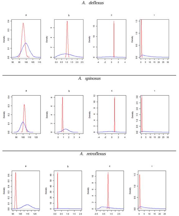
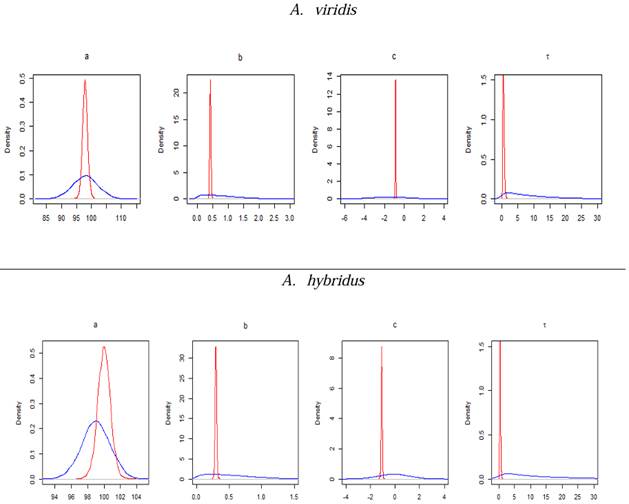
One advantage of Bayesian inference is the ability to obtain probability densities for each model parameter (MARTINS FILHO et al., 2008; HAMZA et al., 2021; FERNANDES et al., 2022; AZARIAS et al., 2025). Figures 1 and 2 illustrates the density priors (in blue) and the density posteriors (in red), according to the models adjusted for each species. The density posteriors of the parameter estimates are more concentrated around the mean, compared to the density priors. This behavior suggested that Bayesian inference reduces the uncertainty associated with the parameters by combining the distribution prior and the likelihood, resulting in more accurate estimates.

Figure 1
Density priors (in blue) and density posteriors (in red) of the Groot model for the dose-response data of the weeds A. deflexus, A. retroflexus, and A. spinosus.

Figure 2
Density priors (in blue) and density posteriors (in red) of the Logistic model for the dose-response data of the weeds A. viridis and A. hybridus.

When analyzing the variances of the distribution prior and posterior (Table 5), the posterior distributions have smaller variances for parameters b and c, indicating a gain in precision. For parameter a, the variance priors and posteriors remained close for most species, although the means presented differences.

Table 5
Mean, standard deviation, and maximum posterior density (HPD) range (LL: lower limit and UL: upper limit), of the parameters of the Groot (A. deflexus, A. retroflexus, and A. spinosus) and logistic (A. viridis and A. hybridus) models.

Model	Species	Parameter	Mean	Standard deviation	-------------𝐻𝑃 𝐷 95% ------------
					LL	UL
Groot	A. deflexus	a	97.9276	1.1154	95.7608	100.0003
		b	1.0440	0.0548	0.9447	1.1494
		c	0.6907	0.0250	0.6436	0.7393
		τ	0.5224	0.2211	0.1414	1.0340
	A. spinosus	a	102.1713	1.3028	99.5299	104.6925
		b	0.8213	0.0519	0.7211	0.9232
		c	0.8144	0.0359	0.7472	0.8895
		τ	0.3324	0.1413	0.0848	0.6123
	A. retroflexus	a	98.6490	0.6351	97.4009	99.9071
		b	0.1980	0.0065	0.1861	0.2122
		c	1.0568	0.0394	0.9751	1.1321
		τ	0.6647	0.2806	0.1702	1.2206
Logistic	A. hybridus	a	100.0054	0.7872	98.4706	101.5704
		b	0.2967	0.0126	0.2724	0.3224
		c	-1.097	0.0481	-1.1889	-1.0018
		τ	0.3544	0.1471	0.1044	0.6541
	A. viridis	a	97.8895	0.8796	96.2478	99.7260
		b	0.4216	0.0195	0.3851	0.4606
		c	-0.8745	0.0320	-0.9385	-0.8136
		τ	0.5502	0.2312	0.1391	1.0010

The parameter estimates were summarized using the mean, posterior standard deviation, and HPD interval, all of which are commonly used in Bayesian inference (FERNANDES et al., 2022; SILVA et al., 2022; AZARIAS et al., 2025). These summaries are presented in table 5 for each parameter, based on the selected models and the evaluation criteria described in table 4. Comparisons of estimates were made within each model. For the Groot model, the weeds A. deflexus, A. spinosus, and A. retroflexus were compared. Similarly, for the logistic model, the species A. viridis and A. hybridus were compared.

All parameter estimates were statistically different from zero, as evidenced by HPD intervals that did not include zero (Table 5). Small standard deviations of the estimates indicate that the posterior distributions are more concentrated around the mean, as verified by the densities in figure 1 and 2. These results suggest that both models adequately describe the analyzed data using the Bayesian method with a maximum entropy prior.

SILVA et al. (2022) used maximum entropy priors for the parameters of the Stanford & Smith nonlinear model when investigating the dynamics of organic residue decomposition in soil. BLOETSCHER et al. (2020) demonstrated that predictive Bayesian methods can improve dose-response curves in the quantitative assessment of microbial risk. The results of both studies indicated that Bayesian inference with maximum entropy priors was efficient.

In the dose-response analysis of herbicides, the parameter a represents the difference between the maximum and minimum control achieved by the herbicide, indicating its effectiveness in controlling weeds (FRANCISCHINI et al., 2019; NETTO et al., 2022). The intervals for the parameter a estimates overlapped between species in both models (Table 5). This suggests that herbicide efficacy is similar for the five species studied, with no significant differences in the percentage of maximum control minus the minimum, which exceeded 90%.

However, it is important to note that for A. spinosus, the model estimated a value for the parameter a above 100%, suggesting overestimation. This behavior is common in dose-response curve adjustments, as observed in AZARIAS et al. (2024b), FRANCISCHINI et al. (2019), and RAIMONDI et al. (2015), who obtained similar values when modeling the control of different Amaranthus species. While such results are statistically possible, values above 100% for this parameter are biologically impossible (KESHTKAR et al., 2021).

The parameter b, which corresponds to 50% control in the Groot and logistic models, did not show overlap between the species, i.e., there was a difference in the doses of C₅₀. CARVALHO et al. (2005) and CARVALHO et al. (2006) adjusted the Streibig logistic model, highlighting its main advantage as the ability to directly estimate the C₅₀ parameter, which facilitates biological interpretation of the results. The posterior mean of the herbicide dose-response in weeds was estimated in increasing order as follows: A. retroflexus (0.1980) < A. hybridus (0.2967) < A. viridis (0.4216) < A. spinosus (0.8213) < A. deflexus (1.0440).

NETTO et al. (2022) evaluated the susceptibility of 33 Amaranthus spp populations to chlorimuron, an ALS inhibitor, collected in Goiás, Mato Grosso, and Paraná. Twenty-seven populations were classified as susceptible, with an average C₅₀of 6.08 g ha^-1, while the remaining six were considered resistant, with an average C₅₀ of 69.70 g ha^-1. In addition, the authors conducted a literature review in which they observed that, for susceptible populations, C₅₀ values varied from 0.08 to 10.82 g ha^-1, with an overall average of 3.07 g ha^-1.

Since achieving 100% control in a dose-response context is not always possible, studies usually focus on the dose that provides 50%, 80%, or 90% control. These doses are generally described by C₅₀, C₈₀ and C₉₀ (FRANCISCHINI et al., 2013; RAIMONDI et al., 2015). In this sense, the necessary amounts of herbicide to achieve these levels of control were calculated using the posterior mean values and the inverse of the two models, as presented in table 6.

Table 6
Herbicide doses that provide 50% (C₅₀), 80 (C₈₀), (minimum acceptable level of weed control) and 90% (C₉₀, excellent control) of control in the five weed species, calculated from the inverse of the Groot (A. deflexus, A. retroflexus, and A. spinosus) and logistic (A. viridis, and A. hybridus) models.

Species	C50	C80	C90
A. deflexus	1.1093	9.1586	36.1610
A. retroflexus	0.2033	0.7867	1.8269
A. spinosus	0.7789	3.9888	9.6912
A. viridis	0.4430	2.3378	6.8211
A. hybridus	0.2967	1.0487	2.1945

Table 6 shows that the five evaluated species achieved 50%, 80%, and 90% control with different doses. According to CARVALHO et al. (2006), these results indicated the species’ varying levels of susceptibility when exposed to the herbicide. ALS-inhibiting herbicides cover six chemical families, including sulfonylureas, a group to which trifloxysulfuron-sodium belongs. These products are widely used to manage broadleaf weeds, such as those in the Amaranthus genus, due to their high efficacy at low doses and the selectivity they offer to the main crops (YU & POWLES, 2014).

The order from the weed requiring the highest dose to the weed requiring the lowest dose to achieve 50%, 80%, and 90% control is as follows: A. deflexus > A. spinosus > A. viridis > A. hybridus > A. retroflexus. The species A. deflexus required higher doses of herbicide than the other species to reach the calculated control levels, indicating its greater resistance to trifloxysulfuron-sodium. The recommended dose of trifloxysulfuron-sodium is 7.50 g ha^-1 (FRANCISCHINI et al., 2013). Conversely, A. retroflexus was the least susceptible to the herbicide, requiring a dose of 1.42 g ha^-1 to achieve 90% control.

FRANCISCHINI et al. (2014) analyzed seven biotypes of A. viridis from different regions and observed variations in the C₅₀ and C₈₀ doses, confirming resistance to trifloxysulfuron-sodium in samples collected in Bahia. C₅₀ values ranged from 0.017 to 12.30 g ha^-1, and C₈₀ values ranged from 0.039 to 61.80 g ha^-1. These ranges encompass biotypes that are both more susceptible and more resistant than those found in this study, whose C₅₀ values ranged from 0.2033 to 1.1093 g ha^-1 and whose C₈₀ values ranged from 0.7867 to 9.1586 g ha^-1.

FRANCISCHINI et al. (2019) investigated the resistance of eight A. retroflexus biotypes suspected of being resistant to the herbicide trifloxysulfuron-sodium. These biotypes were collected in three cotton-producing states in Brazil. They calculated C₉₀ values and found that the estimated doses were undefined for most biotypes, indicating the need for application rates higher than 0.03 kg g ha^-1 to achieve 90% control. This value is more than four times higher than the recommended dose for managing this species.

These results align with Brazilian records identifying cases of multiple Amaranthus herbicide resistance. In cotton crops, A. retroflexus and A. viridis have demonstrated resistance to pyrithiobac-sodium, trifloxysulfuron-sodium, atrazine, and prometryne. Additionally, A. viridis showed resistance to the latter three herbicides (HEAP, 2020; YANNICCARI et al., 2023). A. hybridus has been found to be resistant to glyphosate and ALS inhibitors in plantations in the state of Rio Grande do Sul (MATHIONI et al., 2022; LAMEGO et al., 2024).

CONCLUSION

According to the selection criteria used, the Groot model best described the dose-response data for A. deflexus, A. spinosus, and A. retroflexus. The logistic model was deemed the best fit for A. viridis and A. hybridus. There were no significant differences in the percentage of maximum control minus the minimum obtained.

The weeds presented different levels of susceptibility to the herbicide, with increasing doses required to achieve 50% control, as follows: A. retroflexus (0.1980) < A. hybridus (0.2967) < A. viridis (0.4216) < A. spinosus (0.8213) < A. deflexus (1.0440). The same order was observed for the C₈₀ and C₉₀ doses. These results indicate that A. retroflexus is the most susceptible species to the herbicide, while A. deflexus is the least susceptible.

ACKNOWLEDGMENTS

The authors thank Conselho Nacional de Desenvolvimento Científico e Tecnológico (CNPq) and Coordenação de Aperfeiçoamento de Pessoal de Nível Superior (CAPES) for their financial support.

REFERENCES

• ANDRADE FILHO, M. G. et al. Uma abordagem bayesiana para curvas de crescimento com diferentes densidades a priori. Revista Brasileira de Biometria, v.28, n.2, p.161-181, 2010. Available from: <Available from: https://biometria.ufla.br/antigos/fasciculos/v28/v28_n2/A10_Marinho.pdf >. Accessed: Dec. 11, 2024.
  » https://biometria.ufla.br/antigos/fasciculos/v28/v28_n2/A10_Marinho.pdf
• AZARIAS, E. C. P. et al. Fitting nonlinear double sigmoid models to macauba fruit growth data using Bayesian inference. Ciência Rural, v.55, n.9, 2025. Available from: <Available from: https://doi.org/10.1590/0103-8478cr20240448 >. Accessed: Aug. 25, 2025. doi: 10.1590/0103-8478cr20240448.
  » https://doi.org/10.1590/0103-8478cr20240448.» https://doi.org/10.1590/0103-8478cr20240448
• AZARIAS, E. C. P. et al. Study of the growth of Amaranthus weeds using non-linear models. Brazilian Journal of Biometrics, v.42, n.1, p.1-19, 2024a. Available from: <Available from: https://doi.org/10.28951/bjb.v42i1.639 >. Accessed: Dec. 11, 2024. doi: 10.28951/bjb.v42i1.639.
  » https://doi.org/10.28951/bjb.v42i1.639.» https://doi.org/10.28951/bjb.v42i1.639
• AZARIAS, E. C. P. et al. Evaluation of susceptibility of Amaranthus species to the herbicide trifloxysulfuron-sodium using nonlinear models. Observatório de La Economía Latinoamericana, v.22, n.2, p.e3275, 2024b. Available from: <Available from: https://doi.org/10.55905/oelv22n2-125 >. Accessed: Dec. 12, 2024. doi: 10.55905/oelv22n2-125.
  » https://doi.org/10.55905/oelv22n2-125.» https://doi.org/10.55905/oelv22n2-125
• AZARIAS, E. C. P. et al. Use of von Bertalanffy and logistic models in the description of dry mass accumulation of weeds Amaranthus retroflexus and Amaranthus hybridus. Revista Foco, v.16, n.7, p.e2342-e2342, 2023. Available from: <Available from: https://doi.org/10.54751/revistafoco.v16n7-038 >. Accessed: Dec. 12, 2024. doi: 10.54751/revistafoco.v16n7-038.
  » https://doi.org/10.54751/revistafoco.v16n7-038.» https://doi.org/10.54751/revistafoco.v16n7-038
• BLOETSCHER, F. et al. Demonstrating the benefits of predictive Bayesian dose-response relationships using six exposure studies of Cryptosporidium parvum. Risk Analysis, v.40, n.11, p.2442-2461, 2020. Available from: <Available from: https://doi.org/10.1111/risa.13552 >. Accessed: Apr. 18, 2025. doi: 10.1111/risa.13552.
  » https://doi.org/10.1111/risa.13552.» https://doi.org/10.1111/risa.13552
• BRITO, I. et al. Sensitivities of Urochloa decumbens plants to glufosinate. Planta Daninha, v.36, p.e018174412, 2018. Available from: <Available from: https://doi.org/10.1590/S0100-83582018360100038 >. Accessed: Nov. 15, 2024. doi. 10.1590/S0100-83582018360100038.
  » https://doi.org/10.1590/S0100-83582018360100038.» https://doi.org/10.1590/S0100-83582018360100038
• CANEDO, I. F. et al. Susceptibilidade diferencial ao herbicida glyphosate e capacidade de rebrota de populações de capim-amargoso. Revista Ceres, v.66, n.1, p.18-25, 2019. Available from: <Available from: https://doi.org/10.1590/0034-737X201966010003 >. Accessed: Nov. 10, 2024. doi: 10.1590/0034-737X201966010003.
  » https://doi.org/10.1590/0034-737X201966010003.» https://doi.org/10.1590/0034-737X201966010003
• CARVALHO, S. J. P. et al. Differential susceptibility of Amaranthus genus weed species to the herbicides trifloxysulfuron-sodium and chlorimuron-ethyl. Planta Daninha, v.24, n.3, p.541-548, 2006. Available from: <Available from: https://doi.org/10.1590/S0100-83582006000300017 >. Accessed: Nov. 11, 2024. doi: 10.1590/S0100-83582006000300017.
  » https://doi.org/10.1590/S0100-83582006000300017.» https://doi.org/10.1590/S0100-83582006000300017
• CARVALHO, S. J. P. et al. Dose-response curves to evaluate the control of weed emergence fluxes by imazapic. Planta Daninha, v.23, n.3, p.535-542, 2005. Available from: <Available from: https://doi.org/10.1590/S0100-83582005000300018 >. Accessed: Dec. 12, 2024. doi: 10.1590/S0100-83582005000300018.
  » https://doi.org/10.1590/S0100-83582005000300018.» https://doi.org/10.1590/S0100-83582005000300018
• CARVALHO, S. J. P. et al. Detection of glyphosate-resistant palmer amaranth (Amaranthus palmeri) in agricultural areas of Mato Grosso, Brazil. Planta Daninha, v.33, n.3, p.579-586, 2015. Available from: <Available from: https://doi.org/10.1590/S0100-83582015000300020 >. Accessed: Dec. 12, 2024. doi: 10.1590/S0100-83582015000300020.
  » https://doi.org/10.1590/S0100-83582015000300020.» https://doi.org/10.1590/S0100-83582015000300020
• CARVALHO, D. T. de et al. Uma abordagem bayesiana para modelar a isoterma de langmuir. Brazilian Journal of Biometrics, Lavras, v.35, n.2, p.376-401, 2017. Available from: <Available from: https://biometria.ufla.br/index.php/BBJ/article/view/116 >. Accessed: Oct. 20, 2024.
  » https://biometria.ufla.br/index.php/BBJ/article/view/116
• CUNHA, A. Modeling and quantification of physical systems uncertainties in a probabilistic framework. In: Probabilistic prognostics and health management of energy systems, Springer, p.127-156, 2017. Available from: <Available from: https://doi.org/10.1007/978-3-319-55852-3_8 >. Accessed: Oct. 20, 2024. doi: 10.1007/978-3-319-55852-3_8.
  » https://doi.org/10.1007/978-3-319-55852-3_8.» https://doi.org/10.1007/978-3-319-55852-3_8
• DA SILVA RIBEIRO, L. H. M. et al. Bayesian Modelling of the effects of nitrogen doses on the morphological characteristics of braquiaria grass. Revista Agro@mbiente Online, v.12, n.4, p.245-257, 2018. Available from: <Available from: https://doi.org/10.18227/1982-8470ragro.v12i4.5166 >. Accessed: Oct. 20, 2024. doi: 10.18227/1982-8470ragro.v12i4.5166.
  » https://doi.org/10.18227/1982-8470ragro.v12i4.5166.» https://doi.org/10.18227/1982-8470ragro.v12i4.5166
• DE OLIVEIRA PALA, L. O. et al. Analysis of Count Time Series: A Bayesian GARMA (p, q) Approach. Austrian Journal of Statistics, v.52, n.5, p.131-151, 2023. Available from: <Available from: https://doi.org/https://doi.org/10.17713/ajs.v52i5.1568 >. Accessed: Dec. 12, 2024. doi: 10.17713/ajs.v52i5.1568.
  » https://doi.org/10.17713/ajs.v52i5.1568.» https://doi.org/https://doi.org/10.17713/ajs.v52i5.1568
• DRAPER, N. R.; SMITH, H. Applied Regression Analysis. 3^rd ed. John Wiley & Sons, 1998. v.326. 736 p.
• FERNANDES, T. J. et al. Bayesian estimation of nonlinear models parameters in the description of growth coffee fruits. Brazilian Journal of Biometrics, v.40, n.4, p.393-406, 2022. Available from: <Available from: https://doi.org/10.28951/bjb.v40i4.623 >. Accessed: Nov. 15, 2024. doi: 10.28951/bjb.v40i4.623.
  » https://doi.org/10.28951/bjb.v40i4.623.» https://doi.org/10.28951/bjb.v40i4.623
• FRAGA, D. et al. Changes in the metabolism of soybean plants submitted to herbicide application in different weed management systems. Planta Daninha, v.38, p.e020215525, 2020. Available from: <Available from: https://doi.org/10.1590/S0100-83582020380100043 >. Accessed: Nov. 15, 2024. doi: 10.1590/S0100-83582020380100043.
  » https://doi.org/10.1590/S0100-83582020380100043.» https://doi.org/10.1590/S0100-83582020380100043
• FRANCISCHINI, A. C. et al. Multiple-and cross-resistance of Amaranthus retroflexus to acetolactate synthase (ALS) and photosystem II (PSII) inhibiting herbicides in preemergence. Planta Daninha, v.37, p.e019179353, 2019. Available from: <Available from: https://doi.org/10.1590/S0100-83582019370100026 >. Accessed: Nov. 20, 2024. doi: 10.1590/S0100-83582019370100026.
  » https://doi.org/10.1590/S0100-83582019370100026.» https://doi.org/10.1590/S0100-83582019370100026
• FRANCISCHINI, A. C. et al. Dose-response curves and ALS enzyme inhibitor herbicides efficacy of preemergence applications in Amaranthus species. Revista Brasileira de Herbicidas, v.12, n.1, p.68-77, 2013. Available from: <Available from: https://doi.org/10.7824/rbh.v12i1.195 >. Accessed: Nov. 20, 2024. doi: 10.7824/rbh.v12i1.195.
  » https://doi.org/10.7824/rbh.v12i1.195.» https://doi.org/10.7824/rbh.v12i1.195
• FRANCISCHINI, A. C. et al. First report of Amaranthus viridis resistance to herbicides. Planta Daninha, v.32, n.3, p.571-578, 2014. Available from: <Available from: https://doi.org/10.1590/S0100-83582014000300013 >. Accessed: Nov. 20, 2024. doi: 10.1590/S0100-83582014000300013.
  » https://doi.org/10.1590/S0100-83582014000300013.» https://doi.org/10.1590/S0100-83582014000300013
• FRUHAUF, A. C. et al. Description of height growth of hybrid eucalyptus clones in semi-arid region using non-linear models. Brazilian Journal of Biometrics, v.40, n.2, jun. 2022. Available from: Available from: <https://doi.org/10.28951/bjb.v40i2.543 >. Accessed: Nov. 25, 2024. doi: 10.28951/bjb.v40i2.543.
  » https://doi.org/10.28951/bjb.v40i2.543.» <https://doi.org/10.28951/bjb.v40i2.543
• GEWEKE, J. Evaluating the accuracy of sampling-based approaches to the calculations of posterior moments. Bayesian Statistics, Clarendon Press, v.4, p.641-649, 1992. Available from: <Available from: https://doi.org/10.1093/oso/9780198522669.003.0010 >. Accessed: Dec. 12, 2024. doi: 10.1093/oso/9780198522669.003.0010.
  » https://doi.org/10.1093/oso/9780198522669.003.0010.» https://doi.org/10.1093/oso/9780198522669.003.0010
• GURGEL, A. L. C. et al. Mathematical models to adjust the parameters of in vitro cumulative gas production of diets containing preserved Gliricidia. Ciência Rural, v.51, p.e20200993, 2021. Available from: <Available from: https://doi.org/10.1590/0103-8478cr20200993 >. Accessed: Apr. 19, 2025. doi: 10.1590/0103-8478cr20200993.
  » https://doi.org/10.1590/0103-8478cr20200993.» https://doi.org/10.1590/0103-8478cr20200993
• GROOT, J. C. et al. Multiphasic analysis of gas production kinetics for in vitro fermentation of ruminant feeds. Animal Feed Science and Technology, Elsevier, v.64, n.1, p.77-89, 1996. Available from: <Available from: https://doi.org/10.1016/S0377-8401(96)01012-7 >. Accessed: Dec. 12, 2024. doi: 10.1016/S0377-8401(96)01012-7.
  » https://doi.org/10.1016/S0377-8401(96)01012-7.» https://doi.org/10.1016/S0377-8401(96)01012-7
• HAMZA, T. et al. A Bayesian dose-response meta-analysis model: A simulations study and application. Statistical methods in medical research, v.30, n.5, p.1358-1372, 2021. Available from: <Available from: https://doi.org/10.1177/0962280220982643 >. Accessed: Dec. 12, 2024. doi: 10.1177/0962280220982643.
  » https://doi.org/10.1177/0962280220982643.» https://doi.org/10.1177/0962280220982643
• HASANZADEH, S. et al. Modeling of imazethapyr dose and velvetleaf (Abutilon theophrasti Medik) density interaction on red bean (Phaseolus calcaratus L.) and velvetleaf competition. Advances in Weed Science, v.39, p.e0210015, 2021. Available from: <Available from: https://doi.org/10.51694/AdvWeedSci/2021;39:00020 >. Accessed: Dec. 12, 2024. doi: 10.51694/AdvWeedSci/2021;39:00020.
  » https://doi.org/10.51694/AdvWeedSci/2021;39:00020.» https://doi.org/10.51694/AdvWeedSci/2021;39:00020
• HEAP, I. The international herbicide-resistant weed database. 2020. Available from: <Available from: https://www.weedscience.org/Home.aspx >. Accessed: 20 Oct. 2024.
  » https://www.weedscience.org/Home.aspx
• HOLLAND-LETZ, T. et al. Modeling dose-response functions for combination treatments with log-logistic or Weibull functions. Archives of Toxicology, v.94, p.197-204, 2020. Available from: <Available from: https://doi.org/10.1007/s00204-019-02631-2 >. Accessed: Dec. 12, 2024. doi: 10.1007/s00204-019-02631-2.
  » https://doi.org/10.1007/s00204-019-02631-2.» https://doi.org/10.1007/s00204-019-02631-2
• JANE, S. A. et al. Adjusting the growth curve of sugarcane varieties using nonlinear models. Ciência Rural, v.50, n.3, p.e20190408, 2020. Available from: <Available from: http://dx.doi.org/10.1590/0103-8478cr20190408 >. Accessed: Dec. 12, 2024. doi: 10.1590/0103-8478cr20190408.
  » http://dx.doi.org/10.1590/0103-8478cr20190408
• JAYNES, E. T. Information theory and statistical mechanics. Physical Review, APS, v.106, n.4, p.620, 1957. Available from: <Available from: https://doi.org/10.1103/PhysRev.106.620 >. Accessed: Dec. 12, 2024. doi: 10.1103/PhysRev.106.620.
  » https://doi.org/10.1103/PhysRev.106.620.» https://doi.org/10.1103/PhysRev.106.620
• JAYNES, E. T. Probability Theory: The Logic of Science. Cambridge University Press, 2003. 727 p. Available from: <Available from: https://doi.org/10.1017/CBO9780511790423 >. Accessed: Dec. 12, 2024. doi: 10.1017/CBO9780511790423.
  » https://doi.org/10.1017/CBO9780511790423.» https://doi.org/10.1017/CBO9780511790423
• KAPLAN, D. Bayesian Statistics for the Social Sciences. Guilford Publications, 2023. 250p. Available from: <Available from: https:KAPLAN,+D.+Bayesian+Statistics+for+the+Social+Sciences >. Accessed: Dec. 12, 2024.
  » https:KAPLAN,+D.+Bayesian+Statistics+for+the+Social+Sciences
• KESHTKAR, E. et al. Perspective: Common errors in dose-response analysis and how to avoid them. Pest Management Science, Wiley Online Library, v.77, n.6, p.2599-2608, 2021. Available from: <Available from: https://doi.org/10.1002/ps.6268 >. Accessed: Dec. 12, 2024. doi: 10.1002/ps.6268.
  » https://doi.org/10.1002/ps.6268.» https://doi.org/10.1002/ps.6268
• LAMBERT, B. A Student’s Guide to Bayesian Statistics. London: SAGE Publications Ltd, 2018. 520 p. Available from: <Available from: chrome-extension://efaidnbmnnnibpcajpcglclefindmkaj/https://sites.math.rutgers.edu/~zeilberg/EM20/Lambert.pdf >. Accessed: Apr. 18, 2025.
  » chrome-extension://efaidnbmnnnibpcajpcglclefindmkaj/https://sites.math.rutgers.edu/~zeilberg/EM20/Lambert.pdf
• LAMEGO, F. P. et al. Resistance of Amaranthus hybridus to glyphosate: detection, mechanisms involved and alternatives for integrated management. Advances in Weed Science, v.42, p.e020240046, 2024. Available from: <Available from: https://doi.org/10.51694/AdvWeedSci/2024;42/00025 >. Accessed: Apr. 18, 2025. doi: 10.51694/AdvWeedSci/2024;42/00025.
  » https://doi.org/10.51694/AdvWeedSci/2024;42/00025.» https://doi.org/10.51694/AdvWeedSci/2024;42/00025
• LONGHINI, V. Z. et al. Mathematical models for adjustments in the quantification of ammonia volatilization from urea fertilizer applied on tropical pastures. Ciência Rural, v.54, n.5, p.e20230230, 2023. Available from: <Available from: https://doi.org/10.1590/0103-8478cr20230230 >. Accessed: Apr. 18, 2025. doi: 10.1590/0103-8478cr20230230.
  » https://doi.org/10.1590/0103-8478cr20230230.» https://doi.org/10.1590/0103-8478cr20230230
• MA, J. et al. Nonlinear dose-response modeling of high-throughput screening data using an evolutionary algorithm. Dose-Response, v.18, n.2, p.1559325820926734, 2020. Available from: <Available from: https://doi.org/10.1177/1559325820926734 >. Accessed: Oct. 20, 2024. doi: 10.1177/1559325820926734.
  » https://doi.org/10.1177/1559325820926734.» https://doi.org/10.1177/1559325820926734
• MATHIONI, S. M. et al. PCR-based assay to detect the EPSPS TAP-IVS substitution in Amaranthus hybridus. Advances in Weed Science, v.40, p.e20210048, 2022. Available from: <Available from: https://doi.org/10.51694/AdvWeedSci/2022;40:Amaranthus003 >. Accessed: Apr. 18, 2025. doi: 10.51694/AdvWeedSci/2022;40:Amaranthus003.
  » https://doi.org/10.51694/AdvWeedSci/2022;40:Amaranthus003.» https://doi.org/10.51694/AdvWeedSci/2022;40:Amaranthus003
• MARTINS FILHO, S. et al. Bayesian approach in the growth curves of two cultivars of common bean. Ciência Rural, v.38, n.6, p.1516-1521, 2008. Available from: <Available from: https://www.scielo.br/scielo.php?pid=S0103-84782008000600004&script=sci_abstract&tlng=pt >. Accessed: Oct. 25, 2025. doi: 10.1590/S0103-84782008000600004.
  » https://doi.org/10.1590/S0103-84782008000600004.» https://www.scielo.br/scielo.php?pid=S0103-84782008000600004&script=sci_abstract&tlng=pt
• MJOUN, K. 72 Evaluation of different gas production models when applied to ruminants feeds. Journal of Animal Science, v.96, p.37-38, 2018. Available from: <Available from: https://doi.org/10.1093/jas/sky073.070 >. Accessed: Oct. 20, 2024. doi: 10.1093/jas/sky073.070.
  » https://doi.org/10.1093/jas/sky073.070.» https://doi.org/10.1093/jas/sky073.070
• MOROTA, F. K. et al. Weed management in tropical fruit crops: pinapple, banana, coconut, papaya and passion fruit. Revista Brasileira de Herbicidas, v.19, n.1, 2020. Available from: <Available from: https://doi.org/10.7824/rbh.v19i1.656 >. Accessed: Oct. 20, 2024. doi: 10.7824/rbh.v19i1.656.
  » https://doi.org/10.7824/rbh.v19i1.656.» https://doi.org/10.7824/rbh.v19i1.656
• NETTO, A. G. et al. Multiple resistance of Amaranthus palmeri to ALS and EPSPS inhibiting herbicides in the State of Mato Grosso, Brazil. Planta Daninha, v.34, n.3, p.581-587, 2016. Available from: <Available from: https://doi.org/10.1590/S0100-83582016340300019 >. Accessed: Oct. 25, 2024. doi: 10.1590/S0100-83582016340300019.
  » https://doi.org/10.1590/S0100-83582016340300019.» https://doi.org/10.1590/S0100-83582016340300019
• NETTO, A. G. et al. Geographical distribution and resistance level to chlorimuron of Amaranthus spp. populations in the main soybeans producing regions of Brazil. Advances in Weed Science, v.40, n.spe2, p.e020220063, 2022. Available from: <Available from: https://doi.org/10.51694/AdvWeedSci/2022;40:Amaranthus010 >. Accessed: Apr. 18, 2025. doi: 10.51694/AdvWeedSci/2022;40:Amaranthus010.
  » https://doi.org/10.51694/AdvWeedSci/2022;40:Amaranthus010.» https://doi.org/10.51694/AdvWeedSci/2022;40:Amaranthus010
• OLIVEIRA, A. R. D. et al. Control of Cyperus rotundus L. with trifloxysulfuron-sodium in sugar-cane. Revista Ceres, v.57, n.6, p.736-741, 2010. Available from: <Available from: https://doi.org/10.1590/S0034-737X2010000600006 >. Accessed: Oct. 25, 2024. doi: 10.1590/S0034-737X2010000600006.
  » https://doi.org/10.1590/S0034-737X2010000600006.» https://doi.org/10.1590/S0034-737X2010000600006
• PEREIRA, A. A. et al. Bayesian modeling of the coffee tree growth curve. Ciência Rural, v.52, n.9, p.e20210275, 2022. Available from: <Available from: https://doi.org/10.1590/0103-8478cr20210275 >. Accessed: Oct. 10, 2024. doi: 10.1590/0103-8478cr20210275.
  » https://doi.org/10.1590/0103-8478cr20210275.» https://doi.org/10.1590/0103-8478cr20210275
• PLUMMER, M. et al. CODA: convergence diagnosis and output analysis for MCMC. R News, v.6, n.1, p.7-11, 2006. Available from: < Available from: https://www.r-project.org/doc/Rnews/Rnews_2006-1.pdf >. Accessed: Apr. 15, 2025.
  » https://www.r-project.org/doc/Rnews/Rnews_2006-1.pdf
• RAFTERY, A. L.; LEWIS, S. C. Comment: One long run with diagnostics: Implementation strategies for Markov chain. Statistical Science, v.7, n.4, p.493-497, 1992. Available from: <https://doi.org/10.1214/ss/1177011143>. Accessed: Oct. 20, 2024. doi: 10.1214/ss/1177011143.
• RAIMONDI, M. et al. Dose-response curve to soil-applied herbicides and susceptibility evaluation of different Amaranthus species using model identity. Planta Daninha, v.33, p.137-146, 2015. Available from: <Available from: https://doi.org/10.1590/S0100-83582015000100016 >. Accessed: Oct. 20, 2024. doi: 10.1590/S0100-83582015000100016.
  » https://doi.org/10.1590/S0100-83582015000100016.» https://doi.org/10.1590/S0100-83582015000100016
• RITZ, C. Toward a unified approach to dose-response modeling in ecotoxicology. Environmental Toxicology and Chemistry, v.29, n.1, p.220-229, 2010. Available from: <Available from: https://doi.org/10.1002/etc.7 >. Accessed: Oct. 20, 2024. doi: 10.1002/etc.7.
  » https://doi.org/10.1002/etc.7.» https://doi.org/10.1002/etc.7
• SARI, B. G. et al. Nonlinear modeling for analyzing data from multiple harvest crops. Agronomy Journal, v.110, n.6, p.2331-2342, 2018. Available from: <Available from: https://acsess.onlinelibrary.wiley.com/doi/abs/10.2134/agronj2018.05.0307 >. Accessed: Oct. 20, 2024. doi: 10.2134/agronj2018.05.0307.
  » https://doi.org/10.2134/agronj2018.05.0307.» https://acsess.onlinelibrary.wiley.com/doi/abs/10.2134/agronj2018.05.0307
• SCHOOT, R. V. D. et al. Bayesian statistics and modelling. Nature Reviews Methods Primers, Nature Publishing Group UK London, v.1, n.1, p.1, 2021. Available from: <Available from: https://doi.org/10.1038/s43586-020-00001-2 >. Accessed: Nov. 15, 2024. doi: 10.1038/s43586-020-00001-2.
  » https://doi.org/10.1038/s43586-020-00001-2.» https://doi.org/10.1038/s43586-020-00001-2
• SEBER, G. A.; WILD, C. J. Nonlinear regression. Hoboken, New Jersey: John Wiley and Sons, Inc, 1989. 768 p. Available from: <Available from: https://archive.org/details/nonlinearregress0000sebe/page/n7/mode/2up >. Accessed: Oct. 20, 2024.
  » https://archive.org/details/nonlinearregress0000sebe/page/n7/mode/2up
• SHANNON, C. E. A mathematical theory of communication. The Bell System Technical Journal, Nokia Bell Labs, v.27, n.3, p.379-423, 1948. Available from: <Available from: https://doi.org/10.1002/j.1538-7305.1948.tb01338.x >. Accessed: Nov. 15, 2024. doi: 10.1002/j.1538-7305.1948.tb01338.x.
  » https://doi.org/10.1002/j.1538-7305.1948.tb01338.x.» https://doi.org/10.1002/j.1538-7305.1948.tb01338.x
• SHAO, K. et al. Using Prior Toxicological data to support Dose-Response Assessment─ Identifying Plausible Prior Distributions for Dichotomous Dose-Response Models. Environmental science & technology, v.56, n.22, p.16506-16516, 2022. Available from: <Available from: https://doi.org/10.1021/acs.est.2c05872 >. Accessed: Dec. 12, 2024. doi: 10.1021/acs.est.2c05872.
  » https://doi.org/10.1021/acs.est.2c05872.» https://doi.org/10.1021/acs.est.2c05872
• SILVA, E. M. et al. Método de Newton e Gauss-Newton na estimação dos parâmetros de modelo de regressão não linear. Sigmae, v.8, n.2, p.728-734, 2019. Available from: <Available from: https://10.29327/2520355.8.2-75 >. Accessed: Dec. 12, 2024. doi: 10.29327/2520355.8.2-75.
  » https://doi.org/10.29327/2520355.8.2-75.» https://10.29327/2520355.8.2-75
• SILVA, E. M. et al. Stanford & Smith nonlinear model in the description of CO₂ evolved from soil treated with swine manure: maximum entropy prior. Acta Scientiarum. Technology, v.45, p.e56360-e56360, 2022. Available from: <Available from: https://doi.org/10.4025/actascitechnol.v45i1.56360 >. Accessed: Dec. 12, 2024. doi: 10.4025/actascitechnol.v45i1.56360.
  » https://doi.org/10.4025/actascitechnol.v45i1.56360.» https://doi.org/10.4025/actascitechnol.v45i1.56360
• SILVA, N. R. et al. Differential dry mass accumulation in eucalypt and pine exposed to glyphosate. Revista de Ciências Agroveterinárias, v.14, n.2, p.186-190, 2015. Available from: <Available from: https://www.revistas.udesc.br/index.php/agroveterinaria/article/view/5728 >. Accessed: Dec. 16, 2024.
  » https://www.revistas.udesc.br/index.php/agroveterinaria/article/view/5728
• SMITH, B. J. Bayesian output analysis program (BOA): An R Package for MCMC Output Convergence Assessment and Posterior Inference. Journal of Statistical Software, v.21, n.11, p.1-37, 2007. Available from: <Available from: https://www.jstatsoft.org/article/view/v021i11/0 >. Accessed: Apr. 15, 2025.
  » https://www.jstatsoft.org/article/view/v021i11/0
• STREIBIG, J. C. Herbicide bioassay. Weed Research., v.28, n.6, p.479-484, 1988. Available from: <Available from: https://doi.org/10.1111/j.1365-3180.1988.tb00831.x >. Accessed: Oct. 20, 2024. doi: 10.1111/j.1365-3180.1988.tb00831.x.
  » https://doi.org/10.1111/j.1365-3180.1988.tb00831.x.» https://doi.org/10.1111/j.1365-3180.1988.tb00831.x
• TAKAHASHI, G. O. et al. Control of voluntary soybean plants with herbicides recommended for cotton. Revista Brasileira de Herbicidas, v.19, n.4, p.707, 2020. Available from: <Available from: https://doi.org/10.7824/rbh.v19i4.707 >. Accessed: Dec. 10, 2024. doi: 10.7824/rbh.v19i4.707.
  » https://doi.org/10.7824/rbh.v19i4.707.» https://doi.org/10.7824/rbh.v19i4.707
• R CORE TEAM. R: A Language and Environment for Statistical Computing. R Foundation for Statistical Computing, Vienna, Austria. 2024. Available from: <Available from: https://www.R-project.org/ >. Accessed: Oct. 20, 2024.
  » https://www.R-project.org/
• TESSARO, D. et al. Resistance detection of blackjack to als inhibitors by in vitro plant growth method. Planta Daninha, v.38, p.e020212202, 2020. Available from: <Available from: https://doi.org/10.1590/S0100-83582020380100065 >. Accessed: Dec. 10, 2024. doi: 10.1590/S0100-83582020380100065.
  » https://doi.org/10.1590/S0100-83582020380100065.» https://doi.org/10.1590/S0100-83582020380100065
• TORRES, L. et al. Changes in the physiological characteristics of sugarcane cultivars submitted to herbicide application. Planta Daninha, v.30, n.3, p.581-587, 2012. Available from: <Available from: https://doi.org/10.1590/S0100-83582012000300014 >. Accessed: Oct. 15, 2024. doi: 10.1590/S0100-83582012000300014.
  » https://doi.org/10.1590/S0100-83582012000300014.» https://doi.org/10.1590/S0100-83582012000300014
• TURKMAN, M. A. A. et al. Computational Bayesian statistics: an introduction. Cambridge University Press, 2019. v.11, 228 p. Available from: <Available from: https://doi.org/10.1017/9781108646185 >. Accessed: Oct. 15, 2024. doi: 10.1017/9781108646185.
  » https://doi.org/10.1017/9781108646185.» https://doi.org/10.1017/9781108646185
• WANG, X. et al. Bayesian regression modeling with INLA. Chapman and Hall/CRC, 2018. 276 p. Available from: <Available from: https://doi.org/10.1201/9781351165761 >. Accessed: Oct. 20, 2024. doi: 10.1201/9781351165761.
  » https://doi.org/10.1201/9781351165761.» https://doi.org/10.1201/9781351165761
• YANNICCARI, M. et al. Global patterns of herbicide resistance evolution in Amaranthus spp.: an analysis comparing species, cropping regions and herbicides. Advances in Weed Science, v.40, p.e0202200037, 2023. Available from: <Available from: https://doi.org/10.51694/10.51694/AdvWeedSci/2022;40:Amaranthus011 >. Accessed: Oct. 15, 2024. doi: 10.51694/10.51694/AdvWeedSci/2022;40:Amaranthus011.
  » https://doi.org/10.51694/10.51694/AdvWeedSci/2022;40:Amaranthus011.» https://doi.org/10.51694/10.51694/AdvWeedSci/2022;40:Amaranthus011
• YANG, L. et al. A universal delayed difference model fitting dose-response curves. Dose-Response, v.19, n.4, p.15593258211062785, 2021. Available from: <Available from: https://doi.org/10.1177/15593258211062 >. Accessed: Oct. 15, 2024. doi: 10.1177/15593258211062.
  » https://doi.org/10.1177/15593258211062.» https://doi.org/10.1177/15593258211062
• YU, Q.; POWLES, S. B. Resistance to AHAS inhibitor herbicides: current understanding. Pest management science, v.70, n.9, p.1340-1350, 2014. Available from: <Available from: https://doi.org/10.1002/ps.3710 >. Accessed: Oct. 20, 2024. doi: 10.1002/ps.3710.
  » https://doi.org/10.1002/ps.3710.» https://doi.org/10.1002/ps.3710
• ZHANG, J. et al. Tolerance of pima and upland cotton to trifloxysulfuron (envoke) herbicide under field conditions. Journal of Cotton Research, Springer, v.4, p.1-9, 2021. Available from: <Available from: https://doi.org/10.1186/s42397-021-00101-8 >. Accessed: Dec. 12, 2024. doi: 10.1186/s42397-021-00101-8.
  » https://doi.org/10.1186/s42397-021-00101-8.» https://doi.org/10.1186/s42397-021-00101-8
• ZORNITTA, C. S. et al. Kinetics of in vitro gas production and fitting mathematical models of corn silage. Fermentation, v.7, n.4, p.298, 2021. Available from: <Available from: https://doi.org/10.3390/fermentation7040298 >. Accessed: Dec. 12, 2024. doi: 10.3390/fermentation7040298.
  » https://doi.org/10.3390/fermentation7040298.» https://doi.org/10.3390/fermentation7040298

• CR-2025-0042.R1
• DATA AVAILABILITY STATEMENT
  This article is an integral part of the first author’s thesis, and the script will be made available once the thesis is completed.
• DECLARATION OF USE OF ARTIFICIAL INTELLIGENCE
  The authors did not employ any artificial intelligence in this study.

Edited by

• ASSOCIATE EDITOR:
  Alessandro Dal’Col Lúcio (0000-0003-0761-4200)

• SCIENTIFIC EDITOR:
  Alberto Cargnelutti Filho (0000-0002-8608-9960)

Data availability

This article is an integral part of the first author’s thesis, and the script will be made available once the thesis is completed.

Publication Dates

• Publication in this collection
  16 Feb 2026
• Date of issue
  2026

History

• Received
  28 Jan 2025
• Accepted
  24 June 2025
• Reviewed
  06 Nov 2025