A Nowcasting System for Hydrometeorological Hazard Assessment of Landslides and Flooding - Part 1: Conceptual Formulation

Um Sistema de Nowcasting para Avaliação de Riscos Hidrometeorológicos de Deslizamentos e Inundações - Parte 1: Formulação Conceitual

Abstract

This study presents a novel very short-term hydro-meteorological forecasting system integrating precipitation data from Hydroestimator/NOAA. The system employs a variational version of the TopModel hydrological model alongside landslide and flood hazard models. Operating in continuous 15-minute cycles, it produces scalar and probabilistic two-dimensional hazard fields to support decision-making during extreme events across the State of Rio de Janeiro, Brazil, at a spatial resolution of 4 km. The evaluation of this system considers performance indicators based on contingency tables. Emphasizing a balanced approach between computational efficiency and product utility, this study aims to provide a robust analysis of the system's predictive capabilities in addressing hydro-meteorological challenges.

Keywords:
Nowcasting; Hydroestimator/NOAA; Hydrometeorological hazards

Resumo

Este trabalho introduz um sistema de previsão hidrometeorológica de curto prazo que incorpora a assimilação de campos de precipitação do Hydroestimator/NOAA. O sistema utiliza uma versão variacional do modelo hidrológico TopModel, juntamente com modelos de risco de deslizamento de terra e enchente. Operando em ciclos contínuos de 15 minutos, o sistema gera campos de risco bidimensionais, tanto escalares quanto probabilísticos, para auxiliar na tomada de decisões durante eventos extremos. A área de previsão abrange o estado do Rio de Janeiro, Brasil, com uma resolução espacial de 4 km. A avaliação deste sistema considera indicadores de desempenho baseados em tabelas de contingência. O sistema foi projetado para manter um bom equilíbrio entre custo computacional e os benefícios dos produtos obtidos. Esta abordagem abrangente visa obter uma análise robusta das capacidades preditivas do sistema no enfrentamento de desafios hidrometeorológicos.

Palavras-chave:
Nowcasting; Hidroestimator/NOAA; Perigos hidrometeorológicos

1 Introduction

Risk assessment involves evaluating hazards arising from meteorological phenomena and human activities, intertwining exposure and inherent vulnerability within affected populations. Particularly in rapidly urbanizing regions, the interplay of social and economic factors assumes pivotal significance. Within the contemporary context of climate change, hydrological hazards like tropical cyclones, regional floods, and mass movements are increasingly prevalent.

Froude (2018) delineates a noticeable uptick in mass movement events from 2004 to 2016, notably correlating mean daily rainfall with landslides in South America, particularly in topographically complex areas. Rainfall-triggered mass movements primarily result from surface water runoff and interstitial water within slopes, exacerbating erosion and soil instability. Hydrological models such as the physically based TopModel enable the simulation of rainfall-runoff dynamics, facilitating regionally calibrated predictions of landslide susceptibility (Beven & Kirkby 1979; Seibert et al. 1997; Beven & Freer 2001; Buytaert 2022). Sharma et al. (2008) emphasize the importance of models accurately reflecting reality while maintaining simplicity. The extraction of topographic features from digital mapping is well-documented in the literature (e.g., Jenson & Domingue 1988; Quinn et al. 1991).

Prior to the development of TopModel, hydrological modeling alternatives primarily employed linear reservoir models, such as tank models. These models generally comprise linear reservoirs coupled in series and parallel configurations. Comparisons between different reservoir organization methods, including tank models in series and the traditional Stanford Watershed Model (SWM), have been extensively discussed in the literature (e.g., Jaiswal et al. 2020). From the perspective of event modeling, linear reservoir models can be deemed equivalent for relatively short periods once their parameters have been calibrated (Beven, 1997).

To evaluate potential landslide risk in Brazil, several empirical methods have been presented in the literature (e.g., Guidicini & Iwasa, 1976; Tatizana et al., 1987 a ; 1987b; Guzzetti et al. 2006; D’Orsi 2016). In particular, Tatizana et al. (1987a; 1987b) established discriminant curves to identify landslide risk conditions in the Serra do Mar coastal range of São Paulo State, Brazil, based on the covariance of hourly, daily, and multi-day rainfall accumulations. This approach extends beyond the risk analysis based on monthly and seasonal accumulations by Guidicini & Iwasa (1976).

Hydrological models serve as indispensable tools for forecasting system behavior and understanding hydrological processes in the surface soil layer. These models rely on inputs such as rainfall and infiltration patterns, watershed topographic characteristics, and soil properties (Devia et al. 2015). Recent advancements, such as global landslide susceptibility mapping by Felsberg et al. (2022) and the development of the Global Landslide Forecasting System by Khan et al. (2022), along with localized approaches like flood risk mapping in São Paulo by Tomás et al. (2022), represent significant strides in hazard assessment and mitigation strategies. However, despite their promise, existing models and systems face challenges in achieving required high spatiotemporal resolution, which limits their effectiveness for real-time risk assessment, especially for localized and short-duration events.

In the present proposition, a coherent set of equations is presented based on variational assimilation of global satellite precipitation estimates at a temporal resolution of 15 minutes and spatial resolution of 4 km.

1.1 Hydrological Modeling with Variational TopModel Distributor

The TopModel distributor, initially tailored for mid-latitude regions characterized by homogeneous rainfall patterns across the surface, primarily varying temporally within the watershed's scope, has seen expanded utilization in tropical settings. Notably, applications in locales such as Venezuela (Gomez & Kavzoglu 2005), Guatemala (Preti & Letterio 2015), and the state of Rio de Janeiro, Brazil, where extreme convective events lead to heterogeneous rainfall distribution, have been documented (Karam et al. 2017).

In response to the need for enhanced predictive accuracy in areas prone to water-induced landslides during extreme rainfall, this research endeavors to adapt the TopModel equation set for use in the State of Rio de Janeiro, focusing on its efficacy in delineating zones of surface saturation and consequent landslide hazards. The revised model integrates considerations of both topographical features and rainfall variability, encompassing spatial and temporal heterogeneity in precipitation rates, to generate a comprehensive rainfall landslide-hazard index for the Metropolitan Area of Rio de Janeiro, characterized by complex terrain.

Previous studies by Siqueira (2017) applied the original TopModel, recoded in FORTRAN-90 at the Laboratory of Esperimental Hydrometeorology of the UFRJ, to assess landslide potential distribution in the state of Rio de Janeiro. Conversely, Sanchez Peña (2018) employed the variational TopModel (Karam et al. 2017) to investigate the heightened landslide hazards resulting from the rapid passage of severe thunderstorms across the hilly terrain of the Metropolitan Area of Rio de Janeiro.

While the application of TopModel has been relatively limited in temperate regions like Northern Europe and the British Isles, where precipitation patterns differ considerably from tropical regions, rainfall-induced mass movements remain prevalent. Despite their availability of dense rainfall gauge networks (Burt 2010; Keller et al. 2015), essential for providing input fields for extended domain models based on TopModel distributions, its utilization in such regions also remains underexplored (Karam et al. 2024).

1.2 Objectives

The primary aim of this study is to elucidate a coherent set of equations utilized in a hydrometeorological hazard nowcasting system, which incorporates variational assimilation of atmospheric forcing within the variational TopModel framework.

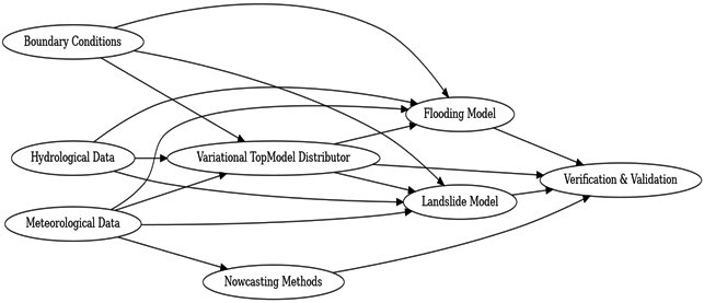
Additionally, leveraging the variational principle allows for the imposition of further constraints on hydrological processes, including differential infiltration, evapotranspiration, and soil heterogeneity. Building upon the work of Karam et al. (2017), who introduced the variational TopModel capable of accommodating rainfall field heterogeneity, our research aims to implement and enhance this approach. Specifically, our system is designed to assess hydrometeorological hazards (landslides and floods) in a subtropical region of Brazil, with a spatial resolution of 4 km and a temporal resolution of 15 minutes, in a continuous mode of operation. Figure 1 illustrates the various components of the numerical system and their interactions. All processes are updated and repeated in short cycles of 15 minutes, producing results sent to a website and framework frontend to allow assessment by potential users.

2 Formulation

In general, water distribution models across the topographic surface necessitate input variables such as the median humidity of the top soil layer, typically an average value that varies solely with time. These median variations are influenced by atmospheric forcing, notably median rainfall in the area, as well as the average energy balance, encompassing surface evapotranspiration.

Figure 1:
Components of the proposed risk model.

2.1 Surface Hydrology Model

The original TopModel, pioneered by Beven & Kirkby (1979), initially emerged as a semi-distributed hydrological model. Its foundational equations are deduced from Darcy's law for vertical hydraulic flow, underpinning the assumption of a linear relationship between hydraulic pressure and the gradient module of topographic slope, coupled with mass continuity considerations. Kirkby (1997) provided a seminal interpretation of the TopModel equations, revealing its derivation from the conservation equation of liquid water volume in the soil integrated along the slope of an elongated drainage strip, adhering to similarity conditions, which are formally expressed by Buckingham's theorem.

In contrast, the dynamic TopModel, as implemented in the R library package, departs from the assumption of similarity and associated optimization, opting instead for solving the continuity equation using finite elements in a 2D grid. This approach accommodates heterogeneities, termed strata layers, allowing for automated processing in R akin to a GIS system. Consequently, the dynamic TopModel represents a distributed version of the original semi-distributed TopModel, tailored to incorporate spatial and temporal variability in atmospheric forcing conditions.

The variational TopModel represents a novel approach to heterogeneous assimilation, leveraging variational analysis principles to accommodate one or more layers of heterogeneities. It formulates a variational problem under weak constraints, leading to the minimization of a functional variational, culminating in a second-order analytical solution typically involving the Helmholtz second-order Partial Differential Equation (PDE), known as the Euler-Lagrange Equation. This framework enables variational assimilation of diverse forces and boundary conditions, elucidating both local and non-local effects resulting from variable atmospheric disturbances over time and space.

Distinguishing between these distribution methods, the original TopModel relies on an invariant spatial structure for the water distribution model, whereas the dynamic version evolves spatially over time, accommodating local effects through the solution of distributed PDEs, generally requiring special methods to solve wave equations (e.g., Durran 2013). On the other hand, the variational TopModel facilitates assimilation of heterogeneous forcing through a continuous and smoothed solution, offering a comprehensive framework for addressing both local and non-local effects in water distribution modeling.

2.2 Variational TopModel Formulation

Water runoff path changes associated with rainfall heterogeneity fields can be defined by a variational principle constraint associated with mass conservation and surface advection of rainfall accumulation (Karam et al., 2017). Let be the variational functional expressed by Equation 1,

$$F=\int {\int }_S\alpha {\left(\lambda -{\lambda }_{\infty }\right)}^2+{\lambda }_E\left(\delta t/{\gamma }_m\right)\left[\partial ln\left(i-j\right)/\partial t+c\cdot \nabla ln\left(i-j\right)\right]ds$$ (1)

where λ is the real topographic index associated with the the real saturation deficit distribution, λ_∞ is the modeled logarithmic topographic index obtained with the original version of TopModel for horizontally homogeneous forcings (such as rainfall, evapotranspiration, upper soil layer discharge, transmissivity, and land cover), α is a normalization coefficient (i.e., the reciprocal of the variance of λ error distribution), λ_E is the scalar Lagrangian function controlling the advection effect on λ, δt is the adjusting time (3600 s), γ_m is the median of the topographic index weighted by the domain area, c .∇ is the advection operator, ds is the area differential, c is the surface runoff velocity, and i and j are the rainfall recharge and discharge of the upper layer of the soil, respectively. The distribution of the asymptotic logarithmic topographic index (λ_∞ ) is obtained through the original TopModel distributor model. The associated Euler-Lagrange Equation is expressed by the Equation 2,

$${\nabla }^2{\lambda }_E+2\alpha \left(\delta t/{\gamma }_m\right)\left[\partial ln\left(i-j\right)/\partial t+c\cdot \nabla ln\left(i-j\right)\right]=0$$ (2)

which is a second-order partial differential equation known as the Helmholtz equation. The correction of λ, which is proportional to the gradient of λ_E , is updated at each time step of 15 min.

2.3 Subsurface Model

In general, water distribution models along the topographic surface require as input variables the median humidity of the top layer of the soil, which is an average value, varies only with time. These median variations are a function of atmospheric forcing (i.e., median rainfall in the area) and also of the average energy balance, which includes surface evapotranspiration. A numerical model composed of linear reservoirs coupled in series was chosen and coded in f90.

Comparisons between the different modes of organization of the reservoirs, for example, tank models in series and traditional Stanford Watershed Model (SWM) have been discussed in the literature (see, for instance, Jaiswal et al. 2020). Such models can be considered equivalent from the point of view of equivalent finality in event modeling, for relatively short periods, once their parameters have been calibrated (Beven, 1997).

This each time step, we vectorized the rainfall field r(x,y,t) to obtaining the associated quantiles distribution and the median value r_med (in m s^-1). Then, we set the maximum infiltration rate, equal to i_max =26×(2.778×10^-7) (in m s^-1). The mean deficit forcing is given by Equation 3,

$$\tilde{D}=exp\left(-4r_{med}/i_{max}\right)$$ (3)

The median deficit is update by the Euler advanced method, as shown in Equation 4,

$$D_{med}=a{D}_{med}+b\tilde{D}$$ (4)

where 𝑏= 𝑑𝑡 𝜏 𝐷 , a=1-b, and 𝜏 𝐷 =10800𝑠 is the time scale (3h). Next, the mean soil wetness is obtained using Equation 5,

$${\alpha }_{med}=1-D_{med}$$ (5)

Then the height of liquid water in the two upper layers of soil is computed following Equation 6,

$${\left(\Delta z_w\right)}_1=h_s^0{\alpha }_{med}{\left(\Delta z_w\right)}_2=h_s^{0}exp\left(-D_{med}\right)$$ (6)

where ℎ 𝑠 0 (m) is the maximum water soil height for each soil layer. Then, the flow density (velocity) discharged from each soil layer (q_i ) (m s^-1) can be computed with help of the time scale 𝜏 𝑖 in (s), 𝑞 𝑖 =𝛥 𝑧 𝑖 𝜏 𝑖 where i = 1, 2 indicates the soil layer level. The base flow density q_b (m s^-1) is equal to q₂ . The total discharge density is q=q₁ +q_b (m s^-1). The median local surface runoff, Runoff_sfc (m s^-1), addressed to riparian recharge is given by Equation 7,

$${Runoff}_{sfc}=max\left\{0.0,\left(R_{lag}-ETp\right)\right\}\times min\left\{tanh\left(3D_m\right),26.0\times \left(2.778\times {10}^{-7}\right)\right\}$$ (7)

The median upper aquifer thickness is given by the total water height in each soil reservoir expressed by Equation 8,

$${\left(\Delta z\right)}_{aquifer}={\left(\Delta z_w\right)}_1+{\left(\Delta z_w\right)}_2$$ (8)

Thus, the total water height above aquifer bedrock is given by Equation 9,

$${watertable}_{deep}=2{watertable}_{deep}^{average}-{\left(\Delta z\right)}_{aquifer}$$ (9)

2.4 Landslide Hazard Model

The stability is a function of the equilibrium condition between two opposite forces: (A) the disruptive tangential force, and (B) the friction force, that resists the disruption and relative movement of layers. The wetting of the soil by precipitation causes both an increase in the density of the soil, with the consequent increase both in the weight of the layer and the shear stress of the inclined terrain, as also this leads to decrease in cohesion, with associated decreasing of the friction force. For a dry soil weight by volume unity γd (in N m^-3), is computed by Equation 10,

$${\gamma }_d=g{\rho }_d$$ (10)

The parameters of the landslide hazard model are shown in Table 1. For the humid soil column, which is the region between the surface and the water table below the soil wetness, the associated non-saturated water deficit is limited to the intervals 𝛼 𝑔 ∈ 0;1 and 𝐷 𝑔 ∈ 0;1 . In contrast, surface water excess is indicated by open intervals 𝛼∈ and 𝐷∈0.0;1.0. The excess water on the soil surface is denoted by 𝛼 𝑒𝑥𝑐𝑒𝑠𝑠 = 𝛼−1 , occurring whenever 𝛼 is greater than to 1, and 𝐷<0, associated with an excess of rainwater accumulated above the soil surface. The soil density variation when the soil is moistened 𝛥𝜌 (kg m^-3) is given by Equation 11,

$$\Delta \rho =\eta {\alpha }_g{\rho }_w$$ (11)

The wet soil density is expressed by Equation 12,

$${\rho }_g={\rho }_d+\Delta \rho$$ (12)

We have to consider effects associated with the soil upper layer volumetric fraction of water or soil upper layer wetness 𝛼 𝑔 and the corresponding soil upper layer water saturation deficit 𝐷 𝑔 , both with values limited to the interval [0; 1]. The excess of water over the surface is obtained always the total water available 𝛼 is larger than soil capacity, expressed in Equation 13.

$${\alpha }_{\text{excess}}=\alpha -1\iff \alpha >1$$ (13)

Table 1.
Parameters of the landslide hazard model. Range ref.: (1) Coelho Netto (1996); (2) Deardorff (1978); (3) Seller (1965); (5) De Blasio (2011); (6) D’Orsi, Feijo & Paes (2002; 2004); D’Orsi (2016), (*) this work.

Par.	Meaning	Values (*)	Usual Range	Unit	Ref.
rscale	Landslide hazard critical rainfall	40	30 - 60	(mm h-1)	(6)
σm	Rainfall margin of the discriminant curve	4	10 - 60	(mm h-1)	(6), (*)
zw	Mean water table depth	3	0.25 - 25	(m)	(2)
ρsd	Mean dry soil density	1600	900 - 2500	(kg m-3)	(3)
tan φ	Mean friction coefficient	1	0.01 - ∞	(-)	(5)
η	Mean soil porosity	0.10	0.01 - 0.45	(-)	(3)

The wet soil density 𝜌 𝑔 (in kg m^-3) considers the replenishing of water by soil pores, as shown by Equation 14.

$${\alpha }_{vol}=\eta {\alpha }_g$$ (14)

Note that 𝛼 𝑣𝑜𝑙 is obtained from the product of porosity 𝜂 and soil upper layer wetness 𝛼 𝑔 . The soil weight by volume unity 𝛾 𝑐 (in N m-3) is computed by Equation 15,

$${\gamma }_c=g{\rho }_g$$ (15)

An estimation of the effective friction coefficient is parameterized by the Equation 16,

$$tan\left({\phi }_{eff}\right)={\phi }_{max}exp\left(-{\alpha }_g\right)$$ (16)

In the function of the soil wetness. The dry soil cohesion (C_d ) (in Pa) is given by Equation 17,

$$C_d=\left({\gamma }_d{z}_w\right)$$ (17)

The cohesion of humid soil (in Pascals) is expressed as shown in Equation 18,

$$C=\left(\gamma z_w\right)$$ (18)

The variation in cohesion resulting from the moistening of the upper soil layer due to rainfall is provided in Equation 19,

$$\Delta C=C-C_d$$ (19)

The normal stress tensor component (in Pa) is calculated using Equation 20,

$$\sigma =\gamma z_w{cos}^2\theta /c_z$$ (20)

Where the denominator is expressed by Equation 21,

$$c_z=c_1{c}_2{c}_3$$ (21)

where the factors are computed by Equation 22,

$$c_1=1,c_2=exp\left(-{\alpha }_g\right)\text{and}{c}_3=exp\left(-sin\theta \right)$$ (22)

The tangential stress tensor component (in Pa) is computed using the Equation 23,

$$\tau =\left({\gamma }_c{z}_w\right)\left(sin\theta cos\theta \right)/c_w$$ (23)

The resistance force (N) in accord with De Blasio (2011) is written as in Equation 24,

$$F_R=\left(\Delta x\Delta y\right)\left(\sigma tan\phi +C\right)$$ (24)

The water height above the surface (m) is estimated by Equation 25,

$$h_{excess}=\left(z_w\eta {\alpha }_g\right)+\left(r\Delta t\right)$$ (25)

The external pressure 𝐶 𝑒 considers only two natural factors: i) the weight force due to the accumulated water depth above the surface; ii) the weight force due to the water excess on the surface from the actual precipitation, Ce , is expressed by Equation 26,

$$C_e=\left(g{\rho }_w\right)\left(h_{scar}\eta {\alpha }_{excess}+r\Delta t\right)$$ (26)

The safety factor is expressed by Equation 27,

$$F=0.9+{\alpha }_0\left({\alpha }_1{\alpha }_2{\alpha }_3{\alpha }_4\right)$$ (27)

where the hazard factors are estimated by Equation 28,

$$\begin{array}{c}{\alpha }_0=exp\left[-\left(tan\theta -tan\phi \right)/tan\phi \right],\\ {\alpha }_1=exp\left(-\Delta {\rho }_s/{\rho }_{sd}\right),\\ {\alpha }_2=exp\left[-{\alpha }_g\right],\\ {\alpha }_3=exp\left(-\Delta C/C_d\right),\\ {\alpha }_4=exp\left(-\Delta C_e/C_d\right).\end{array}$$ (28)

where 𝛥 𝜌 𝑠 and ρ_sd are the wet soil density increment and dry soil density; 𝛼 𝑔 is the volumetric fraction of soil water; 𝛥𝐶 is the wet soil cohesion absolute reduction of the soil cohesion, and 𝛥 𝐶 𝑒 is the external pressure variation associated with the water in excess over the surface and dynamic pressure due to the impact of drops during rainfall. Directly associated is the saturation deficit variation up to rupture, given by Equation 29,

$$\Delta D=F-0.90$$ (29)

With these estimations, the critical rainfall (r_c ) to be provided up to the upper soil layer rupture can be expressed by Equation 30,

$$r_c=r_{scale}{\left[exp\left(\Delta D-1\right)\right]}^{1.1250}$$ (30)

where 𝑟 𝑠𝑐𝑎𝑙𝑒 is the prior value of typical rainfall associated with landslide hazard, locally or regionally defined. In this work, it is equal to 60 mm h^-1, with typical values ranging from 30 to 60 mm h^-1). Finally, the probability of landslides, 𝑃𝑟𝑜𝑏{𝜇}, is given by the following accumulated probability logistic function (as shown in Equation 31),

$$Prob\left\{\mu \right\}=1-1/\left(1+e^{\mu }\right)$$ (31)

The hazard metrics are derived from Equation 32,

$$\mu =\left(r-r_c\right)/{\sigma }_m$$ (32)

where 𝑟 represents the actual rainfall, and 𝜎 𝑚 is the margin of the discriminant risk curve (assumed to be equal to 25% of 𝑟 𝑠𝑐𝑎𝑙𝑒 ). The 𝑃𝑟𝑜𝑏{𝜇} is the cumulative distribution [of probability] function (cdf), obtained by integration of the associated function density of probability between 0 and μ. A landslide hazard mask is used as a binary indicator function, with value 1 is used to indicate a surface element with landslide hazard probability larger than 50% and value 0, otherwise. The parameters used in the present landslide hazard model are based in the literature (e.g., Coelho Netto 1996; Deardorff 1978; Seller 1965; Beven 1997; De Blasio 2011; Gonçalves et al. 2019; and some proposed by this work). The total number of landslides by time step in the simulated area is evaluated using two comparative proxies: the data-based approach, quantified by Equation 33,

$$\left(r{R}_{24h}\right)/\left(3200{mm}^2{h}^{-1}\right)-1$$ (33)

and the model-based approach, estimated through Equation 34,

$$24\text{\%}\left(Prob\mu -0.5\right)$$ (34)

2.5 Flood Risk Assessment

2.5.1 Variable Base Flow Scale and Routing

First, the surface contributing areas of each measurement point 𝑎 𝑥,𝑦,𝑛 along the rivers are determined. The base flow is determined based on this area and different conditioning. It is assumed that the aquifer has a time scale 𝛥 𝑡 𝑎𝑞𝑢𝑖𝑓𝑒𝑟 of 6 hours. The aquifer base flow density scale 𝑄𝑏 𝑘 𝑠𝑐𝑎𝑙𝑒 𝑥,𝑦 into the river, in (m s^-1), is obtained using Equation 35,

$${Qb}_k^{scale}\left(x,y\right)=0.1\eta \left(x,y\right)D_{river}\left(k\right)/\Delta t_{aquifer}+0.0225\sqrt{\left(2g\left(a_{max}-a_{min}\right)\right)}/\Delta t_{aquifer}$$ (35)

where 𝑎 𝑚𝑖𝑛 and 𝑎 𝑚𝑎𝑥 are the minimum and maximum values of the contributing area, and 𝐷 𝑟𝑖𝑣𝑒𝑟 𝑘 is the depth of the riverbank. The flow rate is influenced by various factors in the vicinity of the river section (see Equation 36),

$$\begin{array}{c}{\beta }_2=R_{month}/R_{month}^{scale}\\ {\beta }_3={\left[0.1667W_{river}\left(k\right)\right]}^{1.333}\\ {\beta }_4={\left[0.3333D_{river}\left(k\right)\right]}^{0.1}\\ {\beta }_5=1+0.001z\left(x,y,k\right)\end{array}$$ (36)

where k=1,2,3... is the riverpoint index, 𝛽 1 is the fraction of monthly precipitation 𝑅 𝑚𝑜𝑛𝑡ℎ relative to the climatological maximum (between months), 𝛽 3 is the fraction of river width 𝑊 𝑟𝑖𝑣𝑒𝑟 𝑘 relative to a width scale of 6 m, 𝛽 4 is the potential fraction of river channel height 𝐷 𝑟𝑖??𝑒𝑟 𝑘 relative to a river bank height of 3 m, and 𝛽 5 is the conditional factor of altitude 𝑧 𝑟𝑖𝑣𝑒𝑟 𝑥,𝑦,𝑘 . The contingent base flow 𝑄 𝑏 𝑘 in (m³ s^-1) is given by Equation 37,

$$Qb\left(k\right)=\left({\beta }_2{\beta }_3{\beta }_4{\beta }_5\right){Qb}_k^{scale}{A}_k$$ (37)

where 𝐴 𝑘 is the plain area of the aquifer responsible for local contribution in (m²), typically representing a small fraction of the basin area in rivers confined between mountains and a larger fraction in plain basins.

2.5.2 Surface Runoff Routing

While the assessment of base flow serves as a diagnostic step, the determination of river discharge represents a prognostic phase in this research work.

A numerical analysis is performed to determine the contribution of volumetric surface water flow (in m/s) within the topographical domain, considering water directed towards the river channel point. This assessment not only highlights areas with saturated soil due to rainfall but also pinpoints locations where the precipitation rate surpasses the updated infiltration rate.

A linear transfer function of excess surface water between different points in the watershed is expressed by Equation 38.

$${\lambda }_r\left(x,y,t\right)=exp\left(-\Delta t_{routing}^2/{10800}^2\right)$$ (38)

Where 𝛥 𝑇 𝑟𝑜𝑢𝑡𝑖𝑛𝑔 denotes the estimated water travel time (in s) through particle trajectories from a Particle Dispersion Model (LPD) based on the along-path integration of the stochastic Langevin Equation (Lemons & Gythiel 1997), utilizing velocities obtained from Manning's equation. 𝛥 𝑇 𝑟𝑜𝑢𝑡𝑖𝑛𝑔 is calculated by subtracting the difference in elapsed time between the surface precipitation accumulation (variable in time and space) and the prognosis time (output time series).

The infiltration rate I(x,y,t) in (m s^-1) is determined using the construction method expressed by Equation 39,

$$I\left(x,y,t\right)=0.4R\left(x,y,t\right)exp\left(-4{\alpha }_w\left(x,y,t\right)\right)$$ (39)

Constrained by a minimum value of 𝐼 𝑚𝑖𝑛 =2.778× 10 −9 m s^-1, with a maximum in (m s^-1) determined by the Equation 40,

$$I_{max}=\left(\eta \Delta z_w\right)/\left({nt}_{infiltration}dt\right)$$ (40)

where 𝑛𝑡 𝑖𝑛𝑓𝑖𝑙𝑡𝑟𝑎𝑡𝑖𝑜𝑛 =61.538498 represents the number of time steps of 3600 s required for complete saturation of the soil's surface layer, 𝜂 the soil porosity of surface layer and 𝛥 𝑧 𝑤 is the average water table deep (in m). The infiltration rate 𝐼 𝑥,𝑦,𝑡 in (m s^-1) is given by Equation 41

$$I\left(x,y,t\right)=0.4r\left(x,y,t\right)exp\left(-4{\alpha }_w\left(x,y,t\right)\right)$$ (41)

bounded between the minimum and maximum values.

The water excess on the surface 𝛥 𝑧 𝑠𝑤 (in m) is given by Equations 42 and 43,

$$\Delta z_{sw}^{\text{*}}\left(x,y,t\right)=max\left[0,R\left(x,y,t\right)-I\left(x,y,t\right)\right]\cdot \Delta t$$ (42)

A digital filter is employed to maintain the continuity of surface water, as expressed by the Equation 43,

$$\Delta z_{sw}\left(t\right)=0.2\Delta z_{sw}\left(t-\Delta t\right)+0.8\Delta z_{sw}^{\text{*}}\left(t\right)$$ (43)

The transient flow (perturbation of the base flow) (in m³ s^-1) associated with precipitation from the last hours is obtained through numerical integration as expressed by Equation 44.

$$Q_k^{\text{*}}\left(t\right)={\int }_{t_0}^t{\int }_0^{Lx}{\int }_0^{Ly}{\lambda }_r\left(t,k\right).c\left(k\right).\Delta z_{sw}\left(x,y,t\right).{imap}_{\Delta z_{sw}}\left(x,y\right)dxdydt$$ (44)

The base flow is obtained analogously by calculating the integral given by Equation 45,

$${Qb}^{\text{*}}\left(k\right)={\int }_0^{Lx}{\int }_0^{Ly}{\lambda }_{qb}\cdot c\left(k\right)\cdot Qb\left(k\right)\cdot {imap}_{\Delta z_{sw}}\left(x,y\right)dxdy$$ (45)

Where 𝜆 𝑞𝑏 =1. A digital filter is applied to the river flow, following the Equation 46,

$$Q_k\left(t\right)=0.2Q_k\left(t-1\right)+0.8Q_k^{\text{*}}\left(t\right)$$ (46)

Two innovation functions are defined following Equation 47, used to assess trends.

$$\begin{array}{c}\Delta Q_k^{\text{*}}=Q_k^{\text{*}}\left(t\right)-Q_k^{\text{*}}\left(t-1\right)\\ \Delta Q_b^{\text{*}}=Q_b^{\text{*}}\left(t\right)-Q_b^{\text{*}}\left(t-1\right)\end{array}$$ (47)

2.5.3 Trapezoidal River Section

Base flow and transient flow are incorporated into a numerical routine that models a trapezoidal river section on a slightly inclined plain, both longitudinally and transversely, following the approach proposed by Liu et al. (2015). The distinctive shape of a trapezoidal river section, featuring a flat bottom and sloping sides, significantly influences water flow dynamics. A parameter update table, specific to each monitored river cross-sectional session, is employed to supply the required parameters for calculating time-variable water depth and river width. This calculation applies both when the river is within its banks and when it overflows into the plain. Additionally, kinematic flow, represented by average river velocity, is determined using Manning's formula.

Given the interdependencies among discharge descriptors of rivers (W, H, D, and V) within a generic trapezoidal river section, a numerical solution is obtained through the application of the Newton-Raphson method. Specifically, the bisection algorithm is utilized for root finding.

An implicit numerical solution routine is employed to simultaneously derive the values of flow and water depth in river sections indicated in a look-up table. The session parameters, namely w₁ and w₂ representing the minimum and maximum widths of the primary river channel, h denoting the maximum height of the primary channel, s₁ indicating the longitudinal slope of the river channel, n₁ representing the longitudinal Manning's number of the river, s₂ denoting the average transverse slope of the plain where the river flows, and n₂ being the Manning's number of the plain surface, are provided as input variables to a subroutine (f_riv_var). This subroutine iteratively determines, through the bisection method, the water depth from the base of the river (d) for a given flow modeled by routing excess water overland in the area of influence of the river point. Subsequently, this depth is compared with the containment height capacity of the primary channel to assess overflow conditions from the primary channel to the plain.

Two cases are considered: the first when d is less than h, and the second when d is equal to or greater than h, resulting in the overflow of the primary river channel. In the first case (d<h), the slope angle θ of the river's bank is calculated, in radians, using Equation 48,

$$\theta =atan\left[\left(w_2-w_1\right)/\left(2h\right)\right]$$ (48)

The width (w) of the river's wetted area is obtained using the Equation 49,

$$w=w_1+\left[\left(w_2-w_1\right)/h\right]d$$ (49)

The wetted area is calculated by applying the Equation 50,

$$a_{cross}^{\left(1\right)}=\left[\left(w+w_1\right)/2\right]d$$ (50)

The hydraulic radius (in m) is expressed by the Equation 51,

$$r_1=a_{cross}^{\left(1\right)}/\left(w_1+2d/cos\theta \right)$$ (51)

Alternatively to the Gauckler-Manning-Strickler formula, shown in Equation 52,

$$v_1=r_1^{2/3}{s_1}^{1/2}/n_1$$ (52)

a power relationship (e.g., William, 1978) is applied to obtain the celerity (in m/s) as a function of the discharge (simulated), as expressed by Equation 53,

$$v_1=q_{obs}^{0.30}$$ (53)

The associated flow is calculated by the Equation 54,

$$q_i=v_1{a}_{cross}^{\left(1\right)}$$ (54)

where i is the iteration level of the bisection method, associated with the residue (Equation 55),

$$\left|q_i-q_1\right|<\delta$$ (55)

for a tolerance δ equal to 1 cm. The bisection process is repeated until the condition (Equation 55) is satisfied. If the river depth D is greater than or equal to the height of the primary channel (h), in addition to the variables in the primary channel, variables in the secondary channel (overflow plain) are also calculated, following the iterative bisection process. Similarly, the calculation begins with the determination of the longitudinal slope angle θ (Equation 48), Continuing with the determination of the transverse slope angle of the floodplain (in radians) (Equation 56),

$$\beta =atan\left(s_2\right)$$ (56)

The total width of the river overflowed in the sloping plain is given by the Equation 57,

$$w=w_2+2\left(d-h\right)/s_2$$ (57)

The wetted area is composed of two sub-areas: the first above the primary river section [a_cross ⁽¹⁾], and the second over the plain [a_cross ⁽²⁾], both in (m²), shown in Equation 58,

$$\begin{array}{c}{a}_{cross}^{\left(1\right)}=\left[\left(w+w_1\right)/2\right]d+w_2\left(d-h\right)\\ a_{cross}^{\left(2\right)}={\left(d-h\right)}^2/s_2\end{array}$$ (58)

The corresponding hydraulic radii are expressed (in m) by the Equation 59,

$$\begin{array}{c}{r}_1=a_{cross}^{\left(1\right)}/\left(w_1+2d/cos\theta \right)\\ r_2=a_{cross}^{\left(2\right)}/\left(2\left(d-h\right)/sin\beta \right)\end{array}$$ (59)

Alternatively, the Gauckler-Manning-Strickler formulas (Equation 60),

$$\begin{array}{c}{v}_1=r_1^{2/3}\sqrt{\left(s_1\right)}/n_1\\ v_2=r_2^{2/3}\sqrt{\left(s_2\right)}/n_2\end{array}$$ (60)

The empirical formulas (William, 1978) shown in Equation 61 are employed.

$$\begin{array}{c}{v}_1=q_{obs}^{0.30}\\ v_2=q_{obs}^{0.15}\end{array}$$ (61)

These celerities over the channel and over the flooded plain (in m s^-1) are used to calculate the corresponding flows (Equation 62),

$$\begin{array}{c}{q}_1=v_1{a}_{cross}^{\left(1\right)}\\ q_2=v_2{a}_{cross}^{\left(2\right)}\\ q_i=q_1+q_2\end{array}$$ (62)

The procedure is followed by the bisection method until the residue is sufficiently small.

2.5.4 Flood Hazard Probability

A one-dimensional Gaussian filter convolution is applied to the topography field in both the x and y directions, resulting in a convoluted topography (z_conv). Subsequently, the original topographic field is subtracted from the convoluted one to obtain the two-dimensional distribution of exceeded heights. These heights represent the threshold that must be exceeded for river overflow to occur. It's worth noting that while the Gaussian filter convolution is employed here, it's akin to the more intricate Han's convolution method used for circular boundary frontiers with Fast Fourier Transform (FFT), albeit without the necessity of periodic lateral boundaries.

The local threshold for riverbank overflow Δz_bank is determined by Equation 63, particularly for rivers that are unmonitored and with unknown initial bank heights.

$${\Delta z}_{bank}\left(x,y\right)=z_{conv}\left(x,y\right)-z\left(x,y\right)-min\left\{z_{conv}\right\}+min\left\{z\right\}$$ (63)

For monitored rivers, a lookup table containing river section parameters is utilized. The local water excess on surface is standardized as shown in Equation 64,

$$\mu \left(x,y\right)=\left[{Water}_{Excess}\left(x,y\right)-\Delta z_{bank}\left(x,y\right)\right]/\Delta z_{bank}\left(x,y\right)$$ (64)

The two-dimensional distribution of the Flood Hazard Probability (Prob_F ) (%) is then modeled using a logistic model, as represented in Equation 65,

$${Prob}_F\left(\mu \right)=1-\frac{1}{1+e^{\mu \left(x,y\right)}}$$ (65)

Beyond the evaluation of dimensional values, a categorical distribution can be established to facilitate prompt decision-making. Therefore, a categorical flood risk assessment was formulated for each designated station along selected rivers. This assessment is based on the ratio between water depth (D) within the river channel and the maximum height of the river bank 𝐷 𝑚𝑎𝑥 , which varies depending on the station's position along the stream. A practical proposal for categorizing flood risk is as follows (see Equation 66),

Monitoring (watching): $\frac{D}{D_{max}}<50\text{\%}$,

Warning: $50\text{\%}\le \frac{D}{D_{max}}<80\text{\%}$,

Alert: $80\text{\%}\le \frac{D}{D_{max}}<90\text{\%}$,

High alert: $90\text{\%}\le \frac{D}{D_{max}}<100\text{\%}$,

Overflow (plain-flood): $100\text{\%}\le \frac{D}{D_{max}}$. (66)

This approach categorizes flood risk levels based on the proportion of water depth relative to the maximum height of the river bank at each specific monitoring station. These categories are associated with specific colors and actionable directives for emergency managers. Similar thresholds are currently utilized by the Institute of the Environment of the State of Rio de Janeiro in Brazil (Inea-RJ, 2023).

2.6 Numerical Verifications

In a novel modeling approach, as presented in this work, it is intriguing to consider a scale relation model for validating newly developed methods and magnitudes. For instance, streamflow can be modeled using a scale laws-based model (Williams, 1978), as illustrated in Equation 67,

$$Q^m=V,Q^b=W,Q^f=D$$ (67)

where V is the mean stream velocity (in m s^-1), W is the mean stream width (in m), D is the stream deep (in m), Q is the stream flow (in m³ s^-1), expressed by the product of V, W and D, and m, b, and f are exponents whose summation is unity. The variable Q is obtained at each time step by routing the available surface water flow to the river. Consequently, flow scales V, W and D, obtained from the modeled Q, can be readily applied in verifications.

2.7 Nowcasting

The very short-term forecast (one hour ahead) was generated using an advection method. This method involves estimating the steering flow based on the 2D advection partial differential equation, up to 3 hours in advance. The sequence of precipitation fields from the past 24 hours (each hour) is utilized to estimate the current two-dimensional steering flow vector (i.e., the optical flow). Initially, the approach computes the steering flow using velocity components obtained with the method proposed by Orlansky.

The optical flow was implemented in the modeling system using three methods: Orlanski (1965), Horn and Schunck (1981), and Lucas and Kanade (1981), each followed by self-relaxation smoothing. The first method is considered local, the second variational iterative, and the third of direct solution, using nine points setups.

Optical flows are computed hourly over the preceding 24-hour period and used as input fields (observations) for objective analysis via Barnes interpolation (initially temporal, then spatially) (Barnes 1964; Koch et al. 1983). This approach preserves daily macro-scale flow conditions while capturing details related to the optical displacement of active precipitating systems.

The methodology based on optical flow allows for the transport of precipitation fields to the subsequent hour, maintaining physical consistency with the timing of precipitating systems. Both local variations and structural transport are considered at each time step during the nowcasting period.

The available methods for integrating the advection equation are: 1) the first-order Upwind Method (donor cell method) (Hoffman and Frankel 2018, Mesinger and Arakawa 1976), and 2) the second-order Multidimensional Positively Defined Advective Transport Algorithm (MPDATA) (Smolarkiewicz 2006).

A strategy of filtered time-space based on data time window and Barnes interpolation, realized over time and space, is applied to obtain the Large-scale Advective Optical Flow (24-hour data window), considered the steering flow for rainstorms in the domain area. Therefore, the advective optical flow is retrieved in almost real-time flow, based on the past 24 hours of available fields of precipitation. The structural data window corresponds to the previous 24 hours (with 4 frames per hour) is employed. At regional scale, only the last hour of data is applied to obtain the regional steering optical flow.

The advective nowcasting is obtained each 15 minutes from now to 3 hours in advance. Thus, the local advective optical flow is obtained using data from the previous hour, differently from the South America steering flow obtained with 96 frames during 24 hours (4 frames per hour). The structural data window corresponds to the previous hour (with 4 frames per hour).

The animation of the nowcasting fields: Rainfall [r] (mm h^-1) and Radar reflectivity parameter [dBZ] (dimensionless) are available in the frontend. For that, the NWS-NOAA relationship Z-R is applied as Z = 300 R^1.4, instead of the well-known relationship Z = 200 R^1.6 (Battan, 1973), derived from the drop size distribution (DSD) of Marshall and Palmer (1948). The graphic presents the decibel value of the modeled radar parameter Z, dBZ = 10 log₁₀(Z/1), where the logarithm argument is the ratio between Z (mm⁶ m^-3) and its unit scale. The advective results were obtained using the first-order Upwind Method for the Nowcasting of the Radar reflectivity parameter dBZ and the Rainfall [r] (mm h^-1).

2.7.1 Skill Assessment

Since storms generally move predominantly from West to East in the State of Rio de Janeiro, evaluating the performance of advective nowcasting and persistence focuses on the eastern portion of the domain, where advection time is adequate for storms to traverse half of the zonal domain. Special attention is given to forecasts starting 180 min ago (indicated in the lower right corner of the table), comparing them with the current state. A positive dipole (from lower to higher flow down) centered on the centroid of the current storm indicates excess advective velocity, while a negative dipole (from higher to lower values in the direction of flow) indicates insufficient advective velocity. Thus, the advective velocity range can be finely adjusted using a tuning parameter in the advective program namelist.

2.8 Computational Requirements

The model variants (original, dynamical, and variational) were implemented in Fortran 90 to enhance computational speed and handle large datasets efficiently. The equations were discretized using finite differences, employing advanced schemes in time and centered in space (e.g., Thompson 1961; Mesinger & Arakawa 1976; Marchuk 2012). In the variational TopModel, the solution to the second-order partial differential equation was obtained using the numerical method of sequential relaxation. A five-point two-dimensional Shapiro filter was applied to smooth the forcing. To determine the flow in the cross-section of a measurement point within a river in the hydrographic basin, routing surface water is necessary. Typically, the transport time is illustrated by isochronal lines depicted on the basin map. Here, a Lagrangian constructor method based on the Langevin equation was applied for mapping the transport.

This work presents a set of differential equations used in the conceptual formalization of a comprehensive warning system, specifically an end-to-end Early Warning System (EWS). Coordination among various methods was achieved through a shell-script job, enabling periodic launches, repetition cycles every 15 minutes, and preparation of graphical output. The modeling and parameterization of hazards were grounded in existing technical-scientific knowledge, drawing upon area references, scientific articles, software, and computational source libraries. The system demonstrated its capability to simulate the hazard environment, with associated strata defined by a Specialist Nowcasting System (SPE). This system is customizable and alternatively applied to achieve both high temporal update rates and satisfactory spatial resolution at the mesoscale, seemingly surpassing the capabilities typically offered by Geographic Information Systems (GIS), which are usually tailored for specific time applications. This characteristic holds true irrespective of the format of the two-dimensional field inputs and outputs, which can be in portable universal data formats such as binary with a header file, NetCDF, HDF, etc.

In the context of developing a robust hazard and risk assessment modeling system, several critical requirements have been identified. Firstly, the system must possess the appropriate resolution and versatility to dynamically refocus on the disaster area (known or unknown). This involves the capability for dynamic refocusing into higher-resolution "hazard polygons", as well as support for sub-grids and dynamic downscaling. The system should also demonstrate recursion of the general structure for redirection, ensuring adaptability to evolving scenarios. Furthermore, a comprehensive array of environmental and social management strategies should be established, aligned with the aggravation of the disaster as anticipated by the catastrophe model. Configuration options are pivotal, necessitating a user-friendly interface tailored for technical-scientific operators such as meteorologists, engineers, and geographers. This interface should encompass parametrization and visualization control in namelists, automation of flow data, and sub-grid targeting through recurrence or interaction, with coding facilitated by shell scripts.

Moreover, considerations for portability and low maintenance costs have been prioritized, aligning with the typical features of the Linux environment. The system is expected to operate continuously, requiring automation for 24/7 functionality. Operational frequency, whether hourly updates or every fifteen minutes, should be flexible to accommodate diverse monitoring needs. The dedicated computer hosting the system must exhibit high redundancy and electrical reliability to ensure uninterrupted functionality. In this regard, the placement of web servers should be determined to enhance reliability during events of heavy rain with numerous lightning strikes.

It is crucial to recognize that the final resolution of the model is contingent upon the computational resources available. Hence, scalability and efficiency considerations play a significant role in determining the achievable resolution. Ongoing support and accessibility to users are paramount, emphasizing a commitment to user-friendly interfaces and operational simplicity. This approach ensures that technical-scientific personnel can easily operate and undergo training on the system, contributing to its effective utilization in real-world scenarios.

The current system proposal integrates considerations for landslides and riparian floods as part of a broader effort to develop a comprehensive risk model. This model incorporates layers of vulnerability and exposure, alongside additional hazards such as tropical infectious diseases and severe winds. Additionally, a user-friendly frontend has been designed to enhance user accessibility. The ongoing implementation serves as a proof-of-concept accessible through a website (https://lhydex.igeo.ufrj.br).

The system's performance has been evaluated for landslide and flood events through the analysis of statistical metrics, such as Nash-Sutcliffe Efficiency (NSE), Probability of Detection (POD), and False Alarm Ratio (FAR). Partial and overall assessments have been obtained using Receiver-Operator Curves (ROC). At each time step, 96 frames of 15 minutes each have been analyzed to define conditional probabilities in a contingency table. From these probabilities, various performance metrics have been calculated, including sensitivity and specificity. The overall performance has been assessed by summarizing performance over long periods, resulting in seasonal analyses, for example. High-risk cases have been selected as benchmarks for comparative studies.

3 Results

The effectiveness of the hazard model has been assessed, considering a limited number of severe events observed in the Southeast part of Brazil, which will be further discussed in a companion report. To conduct the verification analysis of hazard conditions, a set of variables obtained from the numerical system, including two-dimensional field perspectives and animations, is transmitted to the model output every 15 minutes (refer to Table 2).

In this initial presentation of the system, demonstrating the validity of the model without the need for presenting specific case studies can be achieved through several approaches. Firstly, the model development was grounded in robust theoretical principles, supported by a comprehensive literature review and the application of well-established methods in the field. Furthermore, conducting detailed comparisons with widely accepted existing models is essential, highlighting the model's performance in controlled simulations and standard conditions. Various versions of the TopModel hydrological model are available for comparison in this context, including the original concentrated version, dynamic distributed version, and the proposed variational version.

The variational version offers advantages over previous iterations by employing more robust routines (elliptical PDEs instead of hyperbolic ones) and producing temporally smoothed risk probability derivatives at an appropriate temporal and spatial resolution for mesoscale risk analysis in rapid update cycles. Sensitivity and uncertainty analyses were also conducted to assess how the model responds to variations in input parameters and how these variations influence model outputs.

Table 2.
The main output variables of the hazard models, updated every 15 minutes, with brackets indicating the potential for exceeding certain values within the usual range.

Variables	Meaning	Usual Range	Unit
Diagnostic variables (available each of last 24 hours):
𝐶 𝑆	Soil cohesion (2D)	(0; 0.7[	105 Pa
𝜏 𝑆	Tangential tensor component (2D) [module]	(0; 2.5[	105 Pa
𝜎 𝑆	Compression tensor component (2D) [module]	(0; 1.4[	105 Pa
𝐹 𝑅	Resistance to be exceeded to rupture (2D) [module]	(0; 2.5[	1012 N
𝐷	Saturation deficit (upper soil layer) (2D)	]-2; 0)	(dimensionless)
𝛼 𝑔	Wetness (upper soil layer) (2D)	(0; 2[	(dimensionless)
F	Safety factor (2D)	(0; 2[	(dimensionless)
𝛥𝑟	Critical rainfall up to soil layer rupture (2D)	(0; 60[	(mm h-1)
𝛥𝐷	Saturation deficit variation up to rupture (2D)	]-2; +2)	(dimensionless)
𝑃𝑟𝑜𝑏 𝐿	Landslide hazard conditional Probability (2D)	(0; 100)	(%)
Prognostic stream variables (available each of next 24 hours):
𝑄 𝑖	River flow(rated points along streams) [module] (1D)	(0; 50000[	(m3 s-1)
𝑞 𝑖	River velocity (points along streams) [module] (1D)	(0.1; 1.3[	(m3 m-2 s-1)
ℎ 𝑖	River water height (rated points along streams) (1D)	(0; 10[	(m)
𝑃𝑟𝑜𝑏 𝐹	Flood hazard conditional Probability (2D)	(0; 100)	(%)
Prognostic stream categorical variables (available each of next 24 hours):
	River overflow status (catchment network) (2D)	5 colors	(countable)

Numerical exploratory tests were carried out to identify an acceptable set of parameters consistent with observed conditions in terms of magnitude and variance, in first approximation. Continuous validation of the model's adherence to known physical principles is crucial to ensure that simulations accurately replicate real hydrological processes.

Currently, the long-term performance of the risk assessment system is under evaluation. Additionally, comparing model results with available general observational data and participating in benchmarking against standard hydrological modeling challenges can provide further evidence of its ability to replicate expected hydrological behavior patterns.

For comparison with other distributed and semi-distributed models, making the core available as an R library is being considered. These combined approaches provide a solid foundation to demonstrate the validity and reliability of the model across different contexts and applications. They serve as an initial step towards advancing research and exploring potential applications.

4 Conclusions

The development of the hydrometeorological hazard modeling system shows promising initial numerical performance, providing rapid risk probabilities and flood analyses at a regional resolution of 4 km, updated every 15 minutes, initially to the State of Rio de Janeiro, Brazil. This capability is crucial for agile decision-making in emergency situations, highlighting the model's relevance for rapid response operations. Integration of different versions of the TopModel hydrological model allowed significant comparisons and sensitivity analyses, revealing advantages in using variational methods that smooth temporal derivatives of risk probability at spatial and temporal scales suitable for mesoscale analysis and risk prediction (nowcasting).

However, continuous caution is required due to uncertainties associated with model parameters and spatial distribution, especially concerning soil heterogeneity. This aspect needs further development to improve prediction accuracy and reduce potential false alarms. Additionally, ongoing validation of the model against known physical principles and comparison with general observational data are essential to ensure simulations accurately replicate real hydrological processes. Collaboration with emergency management centers is crucial to ensure the model's outputs are usable and effective in practical crisis management scenarios.

In summary, this work represents a significant advancement in enhancing the capability to forecast hydrometeorological risks in a regional domain, contributing to informed decision-making in emergency management, particularly through its rapid alert system. It highlights future pathways for improvements and additional applications of the model, emphasizing the importance of addressing identified challenges to maximize its utility and accuracy.

References

• Barnes, S.L. 1964, ‘A technique for maximizing details in numerical weather-map analysis’, Journal of Applied Meteorology, vol. 3, no. 4, pp.396-409.
• Battan, L.J. 1973, Radar Observations of the Atmosphere. University of Chicago Press, Chicago, USA. 324 pp.
• Beven, K.L. & Kirkby, M. 1979, ‘A physically based, variable contributing area model of basin hydrology/Un modèle à base physique de zone d'appel variable de l'hydrologie du bassin versant’, Hydrological Sciences Bulletin, vol. 24, no. 1, pp. 43-69.
• Beven, K.L. (org.). 1997, Advances in Hydrological Processes, vol. 5, no. 1, John Wiley & Sons, New Jersey.
• Beven, K.L. & Freer, J. 2001, ‘A dynamic TopModel’, Hydrol. Process, vol. 15, pp. 1993-2011, DOI: 10.1002/hyp.252.
  » https://doi.org/10.1002/hyp.252.
• Buytaert, W. 2022, TopModel: Implementation of the Hydrological Model TopModel in R, Library R-TopModel, viewed 23 February 2024, < 2022, TopModel: Implementation of the Hydrological Model TopModel in R, Library R-TopModel, viewed 23 February 2024, https://github.com/ICHydro/TopModel >.
  » https://github.com/ICHydro/TopModel
• Burt, S. 2010, ‘British rainfall 1860-1993’, Weather, vol. 65, no. 5, pp. 121-8.
• Coelho Netto, A.L. 1996, ‘Produção de Sedimentos em Bacias Fluviais Florestadas do Maciço da Tijuca, RJ: respostas aos eventos extremos de fevereiro de 1996’, Anais do II Encontro Nacional de Engenharia de Sedimentos, vol. 1, pp. 209-17.
• De Blasio, F.V. 2011, Introduction to the physics of landslides: Lecture notes on the dynamics of mass wasting, Springer Science & Business Media, Germany.
• D’Orsi, R.N., Feijo, L. & Paes, N.M. 2002, ‘Relatório de Escorregamentos’, Fundação Geo-Rio, 58p.
• D’Orsi, R.N., Feijo, R.L. & Paes N.M. 2004, ‘2,500 operational days of Alerta Rio system: History and technical improvements of Rio de Janeiro Warning System for severe weather’, in Lacerda, Ehrlich, Fontoura & Sayão (eds.), Landslides: Evaluation and Stabilization, Taylor & Francis Group, London, pp. 831-36 .
• D’Orsi, R.N. 2016, ‘Lecture about Fundação GeoRio’, AlertaRio System of the Municipality of Rio de Janeiro-RJ, Brazil. 85 slides.
• Deardorff, J.W. 1978, ‘Efficient prediction of ground surface temperature and moisture, with the inclusion of a layer of vegetation’, Journal of Geophysical Research: Oceans, vol. 83, no. C4, pp. 1889-1903.
• Devia, G.K., Ganasri, B.P. & Dwarakish, G.S. 2015, ‘A review on hydrological models’, Aquatic procedia, vol. 4, pp. 1001-7.
• Durran, D.R. 2013, Numerical methods for wave equations in geophysical fluid dynamics, vol. 32, Springer Science & Business Media.
• Felsberg, A., Poesen, J., Bechtold, M., Vanmaercke, M. & De Lannoy, G.J. 2022, ‘Estimating global landslide susceptibility and its uncertainty through ensemble modeling’, Natural Hazards and Earth System Sciences, vol. 22, no. 9, pp. 3063-82.
• Froude, P. 2018, ‘Global fatal landslide occurrence from 2004 to 2016’, Natural Hazards and Earth System Sciences, vol. 18, pp. 2161-81.
• Gomez, H. & Kavzoglu, T. 2005,‘Assessment of shallow landslide susceptibility using artificial neural networks in Jabonosa River Basin, Venezuela’, Engineering Geology, vol. 78, no. 1-2, pp. 11-27.
• Gonçalves, G.C., Escada, M.I.S. & Amaral, S. 2019, ‘Impervious surfaces for population estimate in Brazilian cities’, XIX Simpósio Brasileiro de Sensoriamento Remoto, INPE, Santos-SP, Brasil, pp. 1946-5.
• Guidicini, G. & Iwasa, O.Y. 1976, ‘Correlation Study between Rainfall and Landslides in a Humid Tropical Environment’, Simpósio “Landslides and other Mass Moviment” da IAEG 1977, Praga, Publicação 1080 IPT.
• Guzzetti, F., Reichenbach, P., Ardizzone, F., Cardinali, M. & Galli, M. 2006, ‘Estimating the quality of landslide susceptibility models’, Geomorphology, vol. 81, no. 1-2, pp. 166-184.
• Hoffman, J.D. & Frankel, S. 2018, Numerical methods for engineers and scientists, CRC Press.
• Horn, B.K.P. & Schunck, B.G. (1981). Determining optical flow. Artificial Intelligence, vol. 17, pp.185-203.
• Inea-RJ 2023, Instituto Estadual do Ambiente do Estado do Rio de Janeiro, Brasil, viewed 23 February 2024, <Inea-RJ 2023, Instituto Estadual do Ambiente do Estado do Rio de Janeiro, Brasil, viewed 23 February 2024, http://www.inea.rj.gov.br >.
  » http://www.inea.rj.gov.br
• Jaiswal, R.K., Ali, S. & Bharti, B. 2020, ‘Comparative evaluation of conceptual and physical rainfall-runoff models’, Applied Water Science, vol. 10, no. 1, 48.
• Jenson, S.K. & Domingue, J.O. 1988, ‘Extracting topographic structure from digital elevation data for geographic information system analysis’, Photogrammetric Engineering & Remote Sensing, vol. 54, no. 11, pp. 1593-1600.
• Khan, S., Kirschbaum, D.B., Stanley, T.A., Amatya, P.M. & Emberson, R.A. 2022, ‘Global landslide forecasting system for hazard assessment and situational awareness’, Frontiers in Earth Science, vol. 10, 878996.
• Karam, H.A., Pereira Filho, A.J. & Flores Rojas, J.L. 2017, ‘On the precipitation homogeneity hypothesis in TopModel applications: In Geo-Technologies and Natural Disasters (Special Edition)’, Brazilian Journal of Cartography, vol. 69, no. 1, pp. 13-22.
• Karam, H.A., Blacket, M.A., Silva, R.B.P., Flores Rojas, J.L., Pereira , Filho A.J., Sanchez Peña, C.A., Vásquez Panduro, I.L., Siqueira, B.S. & Angeles Suazo, J.M. 2024, ‘Modeling of Soil Water Distribution in a Small Mid-Latitude Watershed on the British Isle for Short Term Landslide and Flood Risk Assessment’, Anuário do Instituto de Geociências, vol. 1, no. 47, 57297.
• Keller, V.D.J., Tanguy, M., Prosdocimi, I., Terry, J.A., Hitt, O., Cole, S.J., Fry, M., Morris, D.G. & Dixon, H. 2015, ‘CEH-GEAR: 1 km resolution daily and monthly areal rainfall estimates for the UK for hydrological and other applications’, Earth System Science Data, vol. 7, no. 1, pp. 143-155.
• Kirkby, M.J. 1997, ‘TopModel: A Personal View. In Distributed hydrological modeling: application of TopModel concept’, in Beven, K.L. (ed.), ‘Series: Advances in hydrological processes’, John Wiley & Sons.
• Koch, S.E., DesJardins, M., & Kocin, P.J. 1983, ‘An interactive Barnes Objective Map Analysis Scheme for Use with Satellite and Conventional Data’, Journal of Applied Meteorology and Climatology, vol. 22, no. 9, pp. 1487-1503.
• Lemons, D.S., & Gythiel, A. 1997, ‘Paul Langevin's 1908 paper “On the Theory of Brownian Motion”’, American Journal of Physics, Vol. 65, no. 11, pp.1079-1081.
• Liu, G., Schwartz, F.W., Tseng, K.H. & Shum, C.K. 2015, ‘Discharge and water-depth estimates for ungauged rivers: Combining hydrologic, hydraulic, and inverse modeling with stage and water-area measurements from satellites’, Water Resources Research, vol. 51, pp. 6017-35, DOI:10.1002/2015WR016971.
  » https://doi.org/10.1002/2015WR016971.
• Lucas, B.D. & Kanade, T. 1981, ‘An iterative image registration technique with an application to stereo vision’. In Proceedings of Imaging Understanding Workshop, pp. 121-30.
• Marchuk, G. 2012, Numerical methods in weather prediction, Elsevier, Netherlands.
• Marshall, J.S. & Palmer, W.McK. 1948, 'The distribution of raindrops with size', Journal of Meteorology, vol. 5, pp. 165-66.
• Mesinger, F. & Arakawa, A. 1976, Numerical Methods Used in Atmospheric Models, GARP Publications Series, World Meteorological Organization Publication, no. 17, 70p.
• Mesinger, F. & Arakawa, A. 1976, Numerical methods used in atmospheric models, WMO Publication, GARP Publications Series, no. 17, 70p.
• Sanchez Peña, C.A., 2018. ‘Desenvolvimento de um modelo numérico para a avaliação de riscos naturais associados à precipitação na MARJ’, Master’s thesis, Universidade Federal do Rio de Janeiro, Brasil.
• Orlanski, I. 1965, ‘A simple boundary condition for unbounded hyperbolic flows’, Journal of Computational Physics, vol. 21, no. 3, pp. 251-269.
• Preti, F. & Letterio, T. 2015, ‘Shallow landslide susceptibility assessment in a data-poor region of Guatemala (Comitancillo municipality)’, Journal of Agricultural Engineering, vol. 46, no. 3, pp. 85-94.
• Quinn, P., Beven, K., Chevallier, P. & Planchon, O. 1991, ‘The prediction of hillslope flow paths for distributed hydrological modeling using digital terrain models’, Hydrological Processes, vol. 5, no. 1, pp. 59-79.
• Seller, W.D. 1965, ‘Physical Climatology’, University of Chicago Press.
• Seibert, J.A.N., Bishop, K.H. & Nyberg, L. 1997, ‘A test of TopModel's ability to predict spatially distributed groundwater levels’, Hydrological processes, vol. 11, no. 9, pp. 1131-44.
• Sharma, K.D., Sorooshian, S. & Wheater, H. 2008, Hydrological Modelling in Arid and Semi-Arid Areas. Cambridge University Press, New York.
• Siqueira, B.S. 2017, ‘Investigação do papel da precipitação para análise do risco de deslizamentos de encostas’, Master’s thesis, Universidade Federal do Rio de Janeiro, Brasil.
• Smolarkiewicz, P.K. 2006, ‘Multidimensional positive definite advection transport algorithm: An overview’, International Journal for Numerical Methods in Fluids, vol. 50, no. 10, pp. 1123-44.
• Tatizana, C., Ogura, A.T., Cerri, L.E.S. & Rocha, M.C.M. 1987a, ‘Análise da correlação entre chuvas e escorregamentos na Serra do Mar, município de Cubatão’, Proceedings of the 5th Congresso Brasileiro de Geologia de Engenharia, São Paulo, vol. 2, pp. 225-36.
• Tatizana, C., Ogura, A.T., Cerri, L.E.S. & Rocha, M.C.M. 1987b, ‘Modelamento numérico da análise de correlação entre chuvas e escorregamentos aplicado às encostas da Serra do Mar no município de Cubatão’, Proceedings of Congresso Brasileiro de Geologia de Engenharia (5th), São Paulo, vol. 2, pp. 237-48.
• Thompson, P.D. 1961, Numerical weather analysis and prediction, Macmillan, New York.
• Tomás, L.R., Soares, G.G., Jorge, A.A., Mendes, J.F., Freitas, V.L. & Santos, L.B. 2022, ‘Flood risk map from hydrological and mobility data: A case study in São Paulo (Brazil)’, Transactions in GIS, vol. 26, no. 5, pp. 2341-65.
• Williams, G.P. 1978, Hydraulic Geometry of River Cross Sections - Theory of Minimum Variance, Geological Survey Professional Paper, Washington.

• Funding information
  Not applicable.
• Data availability statement
  The model data and reference datasets used in this study are available from the author upon reasonable request. Additionally, the scripts and code developed for this research can be provided for purposes of scientific collaboration and further development.

Edited by

• Editor-in-chief
  Dr. Claudine Dereczynski

• Associate Editor
  Dr. Fernanda Cerqueira Vasconcellos

Data availability

The model data and reference datasets used in this study are available from the author upon reasonable request. Additionally, the scripts and code developed for this research can be provided for purposes of scientific collaboration and further development.

Publication Dates

• Publication in this collection
  25 Aug 2025
• Date of issue
  2024

History

• Received
  23 Feb 2024
• Accepted
  30 July 2024