A new approach to rock mass classification using machine learning algorithms

Abstract

This paper proposes a new model for rock mass classification, using machine learning techniques. The variables used are often associated with well-known geomechanical classifications. Factor analysis permitted reducing system dimensionality, selecting only the significant variables related to the rock mass quality. The proposed model used the k-medoid clustering technique to create the geomechanical classes, specifically the partitioning around medoids algorithm, unsupervised learning. The results indicated the formation of seven groups, labeled through the interpretation of the variable values in each group. Subsequently, a decision tree was applied to obtain the geomechanical classes defined by k-medoids technique; aiming to present an easy way for new users to apply the proposed rock mass classification. The proposed model is a new approach to deal with rock mass classification problems, decreasing subjectivity, increasing parameter selectivity, reducing the dimensionality of geotechnical databases and optimizing the application of classification systems.

Key words
Rock mass classification; Machine learning methods; Partitioning around medoids; Decision tree; Geomechanical parameters

INTRODUCTION

Rock engineering classification systems play an important role in rock engineering and design (Palmström 2009). The first classification system for rock masses was the Rock Load Classification, proposed by Terzaghi (1946) with the objective of estimating the rock load to be carried by steel arches installed to support a tunnel. Since then, classification systems have been proposed with different applications.

Classification systems present limitations. Some authors studied these limitations. Kanik (2019) evaluated the limitations of the RMR applied in weak rock masses. Jalalifar et al. (2011) discussed limitations regarding subjective uncertainties, indicating class boundaries that are improper for describing the natural gradations of rock quality. Therefore, the application of quantitative methods to reduce these limitations is a desirable aim.

Currently, the use of machine learning to solve mining engineering problems is common such as: mining method selection (Hen et al. 1995, Azadeh et al. 2010); prediction of rock strength parameters (Asadi et al. 2011, Cevik et al. 2011, Contreras et al. 2018, Ferentinou et al. 2012); predict landslide occurrences (Dahal & Lombardo 2023); assessment of rock slope stability conditions (Liu & Chen 2007, Zare Naghadehi et al. 2011, 2013, Ferentinou & Fakir 2018, Zhang et al. 2022); update on rock mass classifications systems (Habibagahi & Katebi 1996, Aydin 2004, Jalalifar et al. 2014, Santos et al. 2020, 2021); and hazard assessment system for open pit mine slopes (Santos et al. 2018); several applications (Ali & Chawathé 2000, Mariusz & Marta 2017).

This paper presents a new approach for rock mass classification through machine learning techniques. The proposed system uses a database with historical cases of rock masses in Brazilian open pit mines. The use of machine learning techniques reduced the subjectivity of the classification system. The applied technique for the formation of clusters is the partitioning around medoids (PAM). Afterwards, the decision trees were used to create a system based on rules, which allows new users to apply the proposed system.

A new rock mass classification rating is achieved to define the rock mass quality, based on the variables proposed by Santos et al. (2020). An unsupervised technique was applied; therefore, the RMR classes were not used. The groups were formed from patterns between the samples, that is, they were clustered by their similarity. Each class was described according to the behavior of the variables included in the group.

MATERIALS AND METHODS

Variables used in the study

Santos et al. (2020) improved on the RMR classification system, using multivariate statistics and artificial intelligence. The authors applied factor analysis to identify underlying factors not observable in the original variables, using the variables of these factors in the classification system, instead of all the RMR variables.

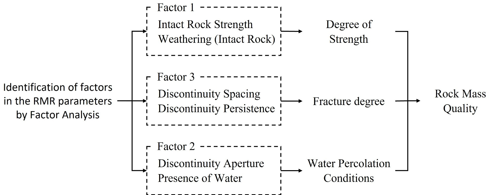
In the previous study by Santos et al. (2020), a factor analysis was applied to the full set of RMR parameters to identify the most influential variables for characterizing rock mass quality. The analysis revealed three main factors: (1) rock strength and weathering, representing the mechanical condition of the intact rock; (2) discontinuity aperture and the presence of water, expressing the hydrogeological influence on rock mass behavior; and (3) discontinuity spacing and persistence, describing the degree of fracturing. These six variables showed the highest communalities and factor loadings, meaning they capture most of the variability in rock mass quality while reducing redundancy. Therefore, they were selected as the input variables in the present study, ensuring both parsimony and representativeness.

The factors identified and interpreted by Santos et al. (2020) have a high relationship with the rock mass quality. For that reason, the variables contained in these factors were used in this present study. Factor 1 is related to the strength of the rock, as it is composed of the intact rock strength and its weathering. Factor 2 is related to the conditions of water percolation in the rock mass, as it includes the presence of water and the discontinuity aperture. Finally, Factor 3 is directly related to the rock mass fracture degree, as it is composed of the variables discontinuity spacing and persistence. The factors are presented in the Figure 1.

Figure 1
Interpretation of Factors identified in the dataset, according to Santos et al. (2020).

Database

A database composed of 3210 samples available in points along mine slopes, encompassing many different open pit mines in Brazil, was used in this study. It is the same data used by Santos et al. (2020).

The database was categorized using the values presented in Table I. The applied ranges correspond to RMR values. Lower ratings in categories refer to situations regarding poor rock mass quality.

Table I
Factors according to Santos et al. (2020).

Intact rock strength
Description	R0	R1	R2	R3	R4	R5	R6
Rating	0	1	2	3	4	5	6
Weathering
Description	W1	W2	W3	W4	W5		W6
Rating	6	5	4	3	2		1
Discontinuity Spacing
Description	> 2 m	0.6 to 2 m	0.2 to 0.6 m	60 to 200 mm		< 60 mm
Rating	5	4	3	2		1
Discontinuity Persistence
Description	< 1 m	1 to 3 m	3 to 10 m	10 to 20 m		> 20 m
Rating	5	4	3	2		1
Discontinuity Aperture
Description	0 mm	< 0.1 mm	0.1 a 1 mm	1 a 5 mm		> 5 mm
Rating	5	4	3	2		1
Water presence
Description		Wet		Dry
Rating		1		5

The intact rock strength (geologist’s hammer test) and rock mass weathering (weathering grades) were evaluated according to ISRM (1981). The parameters of discontinuities were categorized with values from 1 to 5. The presence of water was described by the presence or non-presence of water in each sample.

Methodology

The classes of rock masses were obtained through the application of PAM. Then, a system of rules was created using a decision tree, to obtain these classes from the input database. The decision tree allows the application of the methodology for new database. The Figure 2 presents the general methodology of the study.

Figure 2
General methodology.

The selection of the number of groups was based on the Elbow and Silhouette methods. Thus, each of the grouping possibilities was studied, applying the principle of group interpretability in conjunction with the cluster validation metrics.

An important point for the classification system was the creation of the Score variable (Eq. 1). The Score is the result of the sum of the weights of the variables for each sample in the database under study. Thus, the higher the Score, the higher is the rock mass quality. This “sum” methodology is analogous to the RMR methodology; however, the Score has a smaller number of variables (which are those selected by factor analysis), and the weight system is different.

$\mathrm{Score}=\sum _{i=1}^n{P}_i$ (1)

In Eq. (1), ​​P​​ i​​​​​​ is the value (weight) of variable ​i​​ and ​n​​ is the number of variables of the system, equal to 6. Using the Score and the interpretation of the variable values in each group, it was possible to label the groups (classes, or clusters).

Another important point about the Score was the verification of its relationship with the RMR value in each sampled point. The behavior between the two variables was determined using the correlation coefficient and the equation fitted through the two variables.

A final technique applied in this research was the decision tree. The technique was applied using the results of the clustering model. Thus, through the variables, a decision tree was adjusted to the groups obtained from PAM. The decision tree allowed a visualization of the relationship between the groups. Also, it allows the future use of the classification for new rock masses.

To validate the model, internal and external methods were used. Among the internal methods, we highlight Hopkins statistics, which verifies the tendency of database grouping, the MANOVA statistical test, which verifies whether the clusters are really different groups and, finally, visualization tools to verify the formation of the clusters. For external methods, the interpretability of the clusters was analysed, verifying the distribution of the values of variables in each cluster. In addition, the relationship between the Score and the clusters was verified, which allowed the creation of a hierarchy between clusters.

Repository of codes for applying the methodology.

The software used to apply the techniques was R version 3.3.1 (R Core Team 2019). R is a freeware, permitting the reproduction of the analysis. The packages applied were “cluster” (Maechler et al. 2021) and “rpart” (Therneau et al. 2013) to the PAM and decision tree, respectively.

Theory

K-medoids - partitioning around medoids (PAM) method

Partitioning clustering algorithms have already been popular even before the emergence of data mining (Han et al. 2021). Park & Jun (2009) commented that k-means clustering iteratively finds the k-centroids and assigns every object to the nearest centroid, where the coordinates of each centroid are the mean of the coordinates of the objects in the cluster.

In the problem of rock mass classification, the use of k-medoids is recommended as the variable values are defined by integers (weights). Considering that the medoids are samples extracted from the database, there will never be a weight with decimal places in the centroids. According to Park & Jun (2009) among many algorithms for k-medoids clustering, partitioning around medoids (PAM) proposed by Kaufman & Rousseeuw (1990) is known to be the most powerful.

Similarity measure

For describing similarity measures, consider ​​​ ~ X ​​ i​​​​ = ​​[​x​​ i1​​, ​x​​ i2​​, ​x​​ i3​​, … ​x​​ ip​​​​]​​​ t​​​​, ​i = 1, 2, 3, … , n​​, the vector of observations of variable ​j​​ in individual ​i​​. Being ​​d​​ ij​​​​​​ the distance between individuals ​i​​ and ​j ;​ ​​d​​ ij​​​​​​ only represents a measure of distance if, and only if: (a) ​​d​​ ij​​​​ > 0​ for all ​i​​ and ​j​​; (b) ​​d​​ ij​​​​ = 0​ if, and only if, i = j​​; (c) ​​d​​ ij​​​​ = ​d​​ ji​​​​​​ (d) ​​d​​ ij​​​​ ≤ ​d​​ ik​​​​ + ​d​​ kj​​​​​​ for any individual ​k​​.

The distance measure used in this research is the Euclidean distance. Eq. (2) shows the Euclidean distance between two individuals ​i​​ and ​j​​.

$d_{ij}=\sqrt{{({\tilde{x}}_i-{\tilde{x}}_j)}^t({\tilde{x}}_i-{\tilde{x}}_j)}=\sqrt{\sum _{k=1}^p{(x_{ik}-x_{jk})}^2}$ (2)

PAM algorithm

The PAM algorithm, used in this study, proposed by Johnson & Wichern (2018) is based on the search for k representative objects among the objects of the data set. The PAM algorithm works with the following input: the number of clusters ​k​​ and a database containing ​n​​ objects; and the output: a set of ​k​​ clusters which minimizes a criterion function ​E​​. The algorithm is described by Han et al. (2021) in three steps:

• 1) arbitrarily choose k centers as the initial solution;

• 2) repeat:

  • a) (re)compute membership of the objects according to present solution;

  • b) update some/all cluster centers/distributions according to new membership of the objects;

• 3) until (no change of ​E​​).

For initializing the k-medoids algorithm ​k​​ objects are randomly selected to be the cluster centres. PAM clustering assigns an object to its nearest centre. However, it is performed as part of the process in step 2b of the iterative relocation algorithm making step 2a redundant. This change in centres must result in a decrease of the criterion function ​E​​, according to Han et al. (2021).

To accomplish step 2b, PAM iterates through all the k-cluster centres and tries to replace each of them with one of the other ​​​(​​n − k​​)​​​​ objects. If the squared error function ​E​​ decreases, the replacement takes place, causing the next iteration of algorithm. However, if no replacement happens after going through all k clusters, there is no change of ​E​​, and the algorithm terminates with a local optimum (Han et al. 2021).

Since PAM attempts to replace each of the k cluster centres with one of the ​​​(​​n − k​​)​​​​ objects and each of these attempts results in ​​​(​​n − k​​)​​​​ operations for calculating ​E​​, the total complexity of PAM in one iteration is ​O​​(k ​​(n − k)​​​ 2​)​​. For larger values of ​n​​, such computation becomes costly (Han et al. 2021).

Decision trees

The decision trees model is based on rules, of the “if - else” type, for classification in a tree structure (Kuhn & Johnson 2013). In this research decision tree was used to create the rules to achieve the classes obtained by PAM algorithm.

The model learns by a series of logical decisions, similar to a flowchart, with decision nodes indicating a decision to be made in relation to a variable. The structure is divided into branches that indicate the choices of each decision node. The tree is completed by terminal nodes, also called leaves, which denote the result of following a combination of decisions (Lantz 2015).

There are different measures for selecting the best partition in the decision tree technique. The algorithms seek to divide the data in order to minimize the degree of impurity of the nodes that are in the sequence. Impurity can be understood as the distribution of classes of samples in each node; for example, impurity is null in a node if all the examples in it belong to the same class. Similarly, the maximum degree of impurity in a node occurs if the samples in it are equally distributed between the classes.

Eq. (3) presents one of the measures of impurity, named ​​Inf​​ gain​​​​, ​based on entropy. To determine the quality of a test condition performed, it is necessary to compare the degree of entropy of the parent node (before division) with the degree of entropy of the child nodes (after division). The attribute that gives the biggest difference is chosen as a test condition.

${\mathrm{Inf}}_{gain}=\mathrm{ent}(v_{j-1})-\sum _{j=1}^n[\frac{N(v_j)}{N}\mathrm{ent}(v_j)]$ (3)

In Eq. (3), ​​Inf​​ gain​​​​​​ is the information gained, ​ent​​(​v​​ j−1​​)​​ is the entropy in father node, ​n​​ is the number of attribute values, that is, the number of child nodes, ​N​​ is the total number of objects of the father node and ​N​​(​v​​ j​​​​)​​ is the number of examples associated with the child node ​​v​​ j​​​​​​. Eq. (4) determines the degree of entropy in the node ​​v​​ j​​​​​​, ​ent​​(​v​​ j​​​​)​​.

$\mathrm{ent}(v_j)=-\sum _{i=1}^{k}p(i/v_j)\cdot {log}_2[p(i/v_j)]$ (4)

In Eq. (4), ​p​​(i / ​v​​ j​​​​)​​ is the fraction of the records belonging to class ​i​​ in the node ​​v​​ j​​​​​​, and ​k​​ is the number of classes. This criterion selects the tested attribute that maximizes the information gained.

Another measure is the Gini, which applied a statistical dispersion index proposed in 1912 by the Italian statistician Corrado Gini. The Gini index is used in the CART (Classification and Regression Trees) algorithm proposed by Breiman et al. (1984). It is based on a measure of impurity called gini​​ index​​​​​​. For a problem with ​k​​ classes, the ​​gini​​ index​​​​​​ is defined by Eq. (5).

${\mathrm{gini}}_{index}(v_j)=1-\sum _{i=1}^{k}p{(i/v_j)}^2$ (5)

As in the calculation of the ​​Inf​​ gain​​​​​​, it is enough to calculate the difference between the ​​gini​​ index​​​​​​ before and after the division. This difference, ​Gini​​, is given by Eq. (6). The attribute that generates the highest value for ​Gini​​ is selected.

$\mathrm{Gini}={\mathrm{gini}}_{index}(v_{j-1})-\sum _{j=1}^n[\frac{N(v_j)}{N}{\mathrm{gini}}_{index}(v_j)]$ (6)

Currently, there are several algorithms for decision trees, with emphasis on ID3 (Iterative Dichotomiser 3), proposed by Quinlan (1986), C4.5 (extension of ID3), proposed by Quinlan (1993), and the CART - Classification and Regression Trees, proposed by Breiman et al. (1984).

This research used CART, which is a non-parametric technique. The choice of CART was based on the applicability to the type of data used. In addition, the algorithm does not impose rules in relation to the data set, which adheres to the research objectives.

The main advantages of CART are the ability to search for relationships between data, even when they are not evident, and the production of results in the form of decision trees of great simplicity and easy visualization. The trees generated by the CART algorithm are always binary, which can be traced from their roots to the leaves, answering only simple questions of the type “yes” or “no”. The steps of CART algorithm are:

• i) Initialization at the root node, where the input will be composed of all individuals in the database;

• ii) Split the node in a binary way using the ​Gini​​ criterion;

• iii) Assign to nodes the class to which most individuals belong;

• iv) Finalises the construction of the classification tree using the minimum classification error as a criterion.

RESULTS AND DISCUSSIONS

Determination of the number of groups

The first statistical test applied to the data was the Hopkins statistic, which verifies whether the data tend to group. The value of the Hopkins statistic was 0.33, an average value that indicates the possibility of the database clustering.

The optimal number of classes was determined using the silhouette (Figure 3) and the Elbow methods (Figure 4).

Figure 3
Selection of the number of groups by the Silhouette method.

Figure 4
Selection of the number of groups by Elbow method.

The Elbow method indicates an optimal number of 7 groups. From the silhouette it is possible to see that there is no significant difference between 5, 6 and 7 groups. Therefore, experiments were carried out with the three possibilities, and the choice of 7 groups was the best option based on the principle of group interpretability.

Cluster analysis and validation

Figure 5 shows the result of the silhouette for each sample within each group formed. Although the silhouette has an average value of about 0.30, which means a regular grouping, there are several points with values that reach 0.8; in addition, there are few points with a negative silhouette value.

Figure 5
Silhouette graph for groups.

In Figure 5, the table on the right shows, for each cluster i (​​C​​ j​​​​​​), the number of samples in the cluster (​​n​​ j​​​​​​) and the average silhouette width (​​ave​​ ie​​C​​ j​​​​​​​​​​), which indicates the internal cohesion of each cluster.

Cluster analysis was validated by the statistical tests of MANOVA, presented in Table II. From the results of the tests the null hypothesis is rejected at a confidence level of 99.9%; consequently, the groups formed are statistically different. In Table II, DF is the degrees of freedom.

Table II
MANOVA tests - General Model Adjustment.

Test	DF	Statistical Value	Approximate F	Num. DF	Den. DF	p-value
Pillai	6	1,7917	298.13	30	16015	< 2,2e-16
Wilks	6	0.0472	488.27	30	12798	< 2,2e-16
Hotelling-Lawley	6	7.0668	753.18	30	15987	< 2,2e-16
Roy	6	5,5629	2969.6	6	3203	< 2,2e-16

Visualization of clusters

For visualization of the groups the first 3 principal components (C18, C19 and C20) were plotted, resulting in a representation of a 3-dimensional graph (Figure 6).

Figure 6
Visualization of the groups.

In Figure 6, it is possible to visualize some degree of overlap. However, clusters are quite distinctive and well defined.

This degree of overlap was expected, due to the fact that the cluster analysis aims to assess the rock quality, which is a complex problem. Rock quality can be seen as a transitional problem; within each group there may be overlap.

This is also evident in the supervised models presented by Santos et al. (2020), which showed errors only in neighboring classes. In fact, a sample is included in a group by its multivariate characteristics, which are also defined through ranges of values. Therefore, there is a transition band between the classes of rock, and this is shown in Figure 6.

Interpretation of clusters

The interpretation of the groups was carried out by means of the basic statistics of the variables in each group. The values of number of samples (NS), mean (S1), standard deviation (S2), variance (S3), minimum value (S4), first quartile (S5), median (S6), third quartile (S7), maximum value (S8), mode (S9) and number of samples with value equal to mode (S10) were evaluated. The interpretation of clusters is carried out observing all parameters and comparing them group by group. It is very unlikely in this type of description to find groups with perfect behavior regarding their variables.

Table III presents the values used for interpretation of clusters. In Table III, P1 is the intact rock strength, P2 is the rock weathering, P3 is the discontinuity spacing, P4 is the discontinuity persistence, P5 is the discontinuity aperture and P6 is the presence of water.

Table III
Descriptive statistics for each group.

Variable	Group	NS	S1	S2	S3	S4	S5	S6	S7	S8	S9	S10
P1	1	491	5.88	0.32	0.10	5	6	6	6	6	6	433
P2			5.67	0.47	0.22	5	5	6	6	6	6	329
P3			3.25	0.66	0.44	2	3	3	4	5	3	272
P4			2.05	1.09	1.19	1	1	2	3	5	1	227
P5			3.05	1.45	2.10	1	2	3	5	5	5	145
P6			1	0	0	1	1	1	1	1	1	491
P1	2	1135	4.08	0.91	0.83	2	3	4	5	6	5	399
P2			4.61	0.62	0.38	2	4	5	5	6	5	736
P3			3.09	0.86	0.74	1	3	3	4	5	3	541
P4			1.87	1.08	1.16	1	1	1	3	5	1	632
P5			2.18	1.11	1.24	1	1	2	3	5	2	414
P6			1	0	0	1	1	1	1	1	1	1135
P1	3	340	1.28	0.96	0.91	0	0	1	2	3	2	119
P2			1.98	0.72	0.52	1	1	2	2	4	2	176
P3			3.64	0.74	0.54	2	3	4	4	5	4	172
P4			2.39	1.28	1.64	1	1	3	3	5	1	135
P5			2.40	1.34	1.79	1	1	2	3	5	2	135
P6			1	0	0	1	1	1	1	1	1	340
P1	4	286	1.48	0.68	0.46	0	1	1	2	3	1	149
P2			2.37	0.56	0.32	1	2	2	3	4	2	165
P3			1.13	0.34	0.12	1	1	1	1	2	1	248
P4			1.02	0.20	0.04	1	1	1	1	3	1	283
P5			1.17	0.55	0.30	1	1	1	1	5	1	258
P6			1	0	0	1	1	1	1	1	1	286
P1	5	425	5.06	0.59	0.35	3	5	5	5	6	5	292
P2			5.06	0.48	0.23	4	5	5	5	6	5	325
P3			3.56	0.77	0.59	2	3	4	4	5	4	202
P4			3.51	0.58	0.34	2	3	4	4	5	4	205
P5			1.66	0.90	0.82	1	1	2	2	5	1	211
P6			5	0	0	5	5	5	5	5	5	425
P1	6	315	4.96	0.84	0.71	3	4	5	6	6	5	151
P2			5.25	0.55	0.31	4	5	5	6	6	5	199
P3			3.40	0.89	0.79	2	3	3	4	5	3	165
P4			1.07	0.26	0.07	1	1	1	1	2	1	292
P5			1.90	1.33	1.78	1	1	1	2	5	1	174
P6			5	0	0	5	5	5	5	5	5	315
P1	7	218	2.05	0.67	0.45	1	2	2	2	3	2	120
P2			2.06	0.68	0.47	1	2	2	3	3	2	116
P3			3.59	1.02	1.04	2	3	4	4	5	3	74
P4			2.74	1.29	1.67	1	1	3	4	5	4	72
P5			1.73	0.55	0.31	1	1	2	2	3	2	136
P6			5	0	0	5	5	5	5	5	5	218

The evaluation of the groups was guided by the values presented in Table III. The variables strength and weathering were evaluated by a scale of “high”, “medium” and “low”. The variables spacing, persistence and aperture of discontinuities were analysed together in order to apply an interpretation of the rock mass fracture degree given by a “high”, “medium” and “low” scale.

The PAM technique separated the groups by perfectly discriminating the water variable, that is, there was no mixture of dry and wet conditions. Thus, the variable presence of water was assessed using the following criterion, “wet” or “dry”.

The analysis of the values presented in Table III enabled the description of each class, presented in Table IV.

Table IV
Description of the groups.

Cluster	Description
1	Rock mass with high strength, low weathering, medium fracture. Wet.
2	Rock mass with medium strength, medium weathering, medium fracture. Wet.
3	Rock mass with low strength, high weathering, low fracture. Wet.
4	Rock mass with low strength, high weathering, high fracture. Wet.
5	Rock mass with high strength, low weathering, low fracture. Dry.
6	Rock mass with medium strength, low weathering, medium fracture. Dry.
7	Rock mass with low strength, high weathering, low fracture. Dry.

Creation of the Score variable for class hierarchy

In order to create class hierarchy for the groups formed, the Score variable was proposed (Eq. 1). As previously explained, the Score is the result of the sum of the variable weights for each variable in the database under study.

The Score was calculated for each sample in the database and this value was connected with the groups formed. Figure 7 presents the average values, with minimums and maximums of the Score for each group formed.

Figure 7
Score for each PAM cluster formed.

Analysing Figure 7, it is possible to observe a hierarchy between the groups formed, which reinforces the entire methodology. Thus, with the aid of the average values of the Score and the description of the groups in Table V, it was possible to establish a hierarchy of the groups formed in classes of rock masses. We labeled the groups as classes A to G, with class A representing rock mass with high quality and class G representing rock mass of low quality. The result of this classification is shown in Table V.

Table V
Result of the hierarchy of groups.

Classes	PAM cluster	Score mean
A	5	23.85
B	6	21.57
C	1	20.90
D	7	17.17
E	2	16.83
F	3	12.68
G	4	8.17

Like the RMR classification system, where ranges are established for the values of the classes, we present the ranges for the proposed classes. In Figure 8 and 9 the boxplots for the Score are presented. Rock masses in Figure 8 are dry, while in Figure 9 they are wet.

Figure 9
Score ranges for classes C, E, F and G.

Figure 8
Score ranges for classes A, B and D.

The analysis was performed for the two water conditions (wet and dry), given that the PAM method separated these groups perfectly. A small range of overlap is observed at the extremes of the distributions (see Figure 10 and 11), but in the range between the 1st and 3rd quartiles this overlap is minimal. Therefore, the ranges of classes proposed at this point will be based on the values of the quantiles.

Figure 10
Distribution of the Score for classes A, B and D.

Figure 11
Distribution of the Score for classes C, E, F and G.

Based on Figures 8 to 11, Table VI is proposed with the ranges of Score values for rock mass classification, using the values of the class quantiles. The use of the interval between the 1st and 3rd quartiles indicates a probability value of 0.5 for the rock mass belongs to that labeled class, as this is believed to be a coherent premise to be adopted. Nevertheless, in classes G and A the minimum and maximum possible values were considered to define the extremes of these classes.

Table VI
Proposed ranges for the score variable.

Classes	1st Quartile	3rd Quartile	Water condition
Class A	23	32 (maximum score)	Dry situation
Class B	20	23
Class D	16	19
Class C	20	22	Wet situation
Class E	15	19
Class F	11	14
Class G	5 (minimum score)	10

Relationship between the Score and the RMR

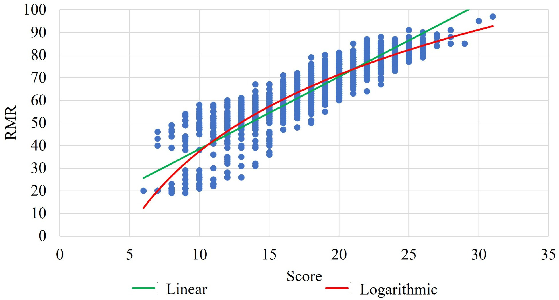
The relationship between the Score and the RMR for each sample in the database was studied. Pearson’s correlation coefficient between the two variables was 0.92, which expresses a strong positive linear relationship. Figure 12 shows the scatterplot between the Score and the RMR.

Figure 12
Relationship between the RMR and the Score.

From Figure 12, a function fitting was proposed between the two variables, a linear function and a logarithmic function. The two functions presented interesting results with the value for the determination coefficient of 0.84 for the linear function, and 0.87 for the logarithmic function.

From the values of the determination coefficient, it is possible to state that the proportion of the RMR variability is explained by the Score, that is, the RMR can be predicted from the Score. Eq. (7) and Eq. (8) are the equations to obtain the RMR from the Score, using linear and logarithmic functions, respectively.

$\mathrm{RMR}=3.20(\mathrm{Score})+6.45\text{with }{R}^2=0.84$ (7)

$\mathrm{RMR}=48.92\ln (\mathrm{Score})-75.23\text{with }{R}^2=0.87$ (8)

Application of decision trees

A classification system using decision rules, specifically the decision tree technique, was applied to the results of cluster analysis. It allowed the visualization of decisions about the variable values in relation to the labeled classes. The decision tree is another way of validating the applied labels and providing an alternative for using the classification system, different from that based only on the description of the rock mass. Figure 13 shows the results of the trained decision tree considering the variables used by grouping through the PAM technique.

Figure 13
Decision tree for the classification according to the groups.

The decision tree presented in Figure 13 was designed with the objective of extracting the maximum amount of information from the groups and allowing a quick and simple application of the proposed system.

For the training and testing of the tree, a sample partition system was not used, that is, the entire database was used to build the tree. The overall accuracy of the decision tree was 0.96.

From Figure 13, it is possible to observe that the system was built discriminating the rock masses based on the presence of water. This result is consistent with the result of cluster analysis which separated the classes from the rock mass by the variable presence of water.

After the presence of water, the variables discontinuity persistence, rock strength and weathering are the most important for discrimination in groups. In the dry rock masses, the importance of discontinuity persistence and weathering is observed, while in the rock masses with water, rock strength and weathering are observed, orienting the nodes for the classification. In rock masses with water at lower levels of the tree, the variables discontinuity spacing and aperture discriminate the classes. In fact, all variables are present in at least one node of the decision tree, which implies that all variables were used by the classification system.

From the decision tree in Figure 13, it is interesting to observe the influence of discontinuity aperture and spacing in wet rock masses. The permeability of rock masses strongly depends on these variables and, according to the decision tree path, they discriminate the classes C, E, F and G.

The poorest class in terms of rock quality, the class G, is strongly influenced by discontinuity spacing. The behaviour of class G is similar to a weathered continuum rock mass, due to the importance of spacing in its definition. According to the decision tree, it is the variable which separates class G from class F.

CONCLUSIONS

The development of mathematical and statistical techniques has contributed to achieve quantitative and less subjective models in rock engineering. In this work, a new approach to rock mass classification using the PAM and decision tree techniques was presented. The proposed model showed high performance and promising results for solving rock classification problems.

The methodology used extensive database, with different rock masses, from poor to high quality ones. The model input parameters were intact rock strength and weathering, presence of water, discontinuity aperture, spacing and persistence.

The proposed model is quantitative, less subjective, formed by a smaller number of variables, comparing to RMR geomechanical classification. Input parameters are variables easily measured in the field. The reduction of variables is advantageous, as it allows field work to be carried out faster, with few sources of errors.

The proposed model helps to classify and clarify the behavior of rock masses. The classification score shows a high relationship with the RMR value, indicating a similar behavior. Though, it is believed that the selectivity of the parameters and the reduction of the data dimensionality allow the simplification of geotechnical surveys without influencing the estimation of the rock mass quality.

The results obtained in this work indicate advances in the subject of rock mass classification. As a suggestion for future work, it is believed that the expansion of the database can contribute to this research, especially concerning the score limits for classes.

Finally, the research was developed using freeware, which allows other users to reproduce the proposed methodology. Therefore, the methodology can be consider an under development approach, allowing for updates and improvements.

Although the mathematics of applied techniques is quite complex, the results are easy to interpret and apply.

Acknowledgements

The authors would like to thank Conselho Nacional de Desenvolvimento Científico e Tecnológico (CNPq), for supporting this work.

• Data availability
  The repository with the codes can be found in github, see the link: https://github.com/allanerlikhman?tab=repositories.

References

• ALI M & CHAWATHÉ A. 2000. Using artificial intelligence to predict permeability from petrographic data. CG 26(8): 915-925. doi: 10.1016/s0098-3004(00)00025-x.
  » https://doi.org/10.1016/s0098-3004(00)00025-x
• ASADI M, EFTEKHARI M & BAGHERIPOUR MH. 2011. Evaluating the strength of intact rocks through genetic programming. Appl Soft Comput 11(2): 1932-1937. doi: 10.1016/j.asoc.2010.06.009.
  » https://doi.org/10.1016/j.asoc.2010.06.009
• AYDIN A. 2004. Fuzzy set approaches to classification of rock masses. Engineering Geology 74(3-4): 227-245. doi: 10.1016/s0013-7952(04)00081-x.
  » https://doi.org/10.1016/s0013-7952(04)00081-x
• AZADEH A, OSANLOO M & ATAEI M. 2010. A new approach to mining method selection based on modifying the Nicholas technique. Appl Soft Comput 10(4): 1040-1061. doi: 10.1016/j.asoc.2009.09.002.
  » https://doi.org/10.1016/j.asoc.2009.09.002
• BREIMAN L, FRIEDMAN JH, OLSHEN R & STONE CJ. 1984. Classification and Regression Trees. Belmont, CA: Wadsworth, p. 368.
• CEVIK A, SEZER EA, CABALAR AF & GOKCEOGLU C. 2011. Modeling of the uniaxial compressive strength of some clay-bearing rocks using neural network. Appl Soft Comput 11(2): 2587-2594. doi: 10.1016/j.asoc.2010.10.008.
  » https://doi.org/10.1016/j.asoc.2010.10.008
• CONTRERAS LF, BROWN ET & RUEST M. 2018. Bayesian data analysis to quantify the uncertainty of intact rock strength. J Rock Mech Geotech Eng 10(1): 11-31. doi: 10.1016/j.jrmge.2017.07.008.
  » https://doi.org/10.1016/j.jrmge.2017.07.008
• DAHAL A & LOMBARDO L. 2023. Explainable artificial intelligence in geoscience: A glimpse into the future of landslide susceptibility modeling. Computers & Geosciences 176: 105364. https://doi.org/10.1016/j.cageo.2023.105364.
  » https://doi.org/10.1016/j.cageo.2023.105364
• FERENTINOU M & FAKIR M. 2018. Integrating Rock Engineering Systems device and artificial neural networks to predict stability conditions in an open pit. Eng Geol 246(28): 293-309. doi: 10.1016/j.enggeo.2018.10.010.
  » https://doi.org/10.1016/j.enggeo.2018.10.010
• FERENTINOU M, HASIOTIS T & SAKELLARIOU M. 2012. Application of computational intelligence tools for the analysis of marine geotechnical properties in the head of Zakynthos canyon, Greece. Computers & Geosciences 40: 166-174. doi: 10.1016/j.cageo.2011.06.022.
  » https://doi.org/10.1016/j.cageo.2011.06.022
• HABIBAGAHI G & KATEBI S. 1996. Rock mass classification using fuzzy sets. IRJST 20: 273-284.
• HAN J, KAMBER M & TUNG AKH. 2021. Spatial clustering methods in data mining: A survey. In: Miller HJ & Han J (Eds), Geographic Data Mining and Knowledge Discovery. Taylor & Francis, p. 1-29.
• HEN X. 1995. A study on the neural network based expert system for mining method selection. Computer Applications and Software, p. 95.
• ISRM - INTERNATIONAL SOCIETY FOR ROCK MECHANICS. 1981. Rock Characterization, Testing and Monitoring – ISRM Suggested Methods. Pergamon Press, Oxford. Available at: https://isrm.net/page/show/177
  » https://isrm.net/page/show/177
• JALALIFAR H, MOJEDIFAR S & SAHEBI AA. 2014. Prediction of rock mass rating using fuzzy logic and multi-variable RMR regression model. Int J Min Sci Technol 24(2): 237-244. doi: 10.1016/j.ijmst.2014.01.015.
  » https://doi.org/10.1016/j.ijmst.2014.01.015
• JALALIFAR H, MOJEDIFAR S, SAHEBI AA & NEZAMABADI-POUR H. 2011. Application of the adaptive neuro-fuzzy inference system for prediction of a rock engineering classification system. Computers & Geotechnics 38(6): 783-790. doi: 10.1016/j.compgeo.2011.04.005.
  » https://doi.org/10.1016/j.compgeo.2011.04.005
• JOHNSON RA & WICHERN DW. 2018. Applied Multivariate Statistical Analysis. Pearson, 6th ed., p. 808.
• KANIK M. 2019. Evaluation of the limitations of RMR89 system for preliminary support selection in weak rock class. Computers & Geotechnics 115: 103159. doi: 10.1016/j.compgeo.2019.103159.
  » https://doi.org/10.1016/j.compgeo.2019.103159
• KAUFMAN L & ROUSSEEUW PJ. 1990. Finding Groups in Data: An Introduction to Cluster Analysis. New York, John Wiley & Sons. DOI: 10.2307/2532178.
• KUHN M & JOHNSON K. 2013. Applied Predictive Modeling. Springer, New York, p. 600. https://doi.org/10.1007/978-1-4614-6849-3
  » https://doi.org/10.1007/978-1-4614-6849-3
• LANTZ B. 2015. Machine Learning with R. Birmingham. Packt Publishing Ltd, Birmingham, UK, p. 452.
• LIU YC & CHEN CS. 2007. A new approach for application of rock mass classification on rock slope stability assessment. Engineering Geology 89(1-2): 129-143. doi: 10.1016/j.enggeo.2006.09.017.
  » https://doi.org/10.1016/j.enggeo.2006.09.017
• MAECHLER M, ROUSSEEUW P, STRUYF A, HUBERT M & HORNIK K. 2021. cluster: Cluster Analysis Basics and Extensions. R package version 2.1.1. Available at: https://www.researchgate.net/publication/272176869_Cluster_Cluster_Analysis_Basics_and_Extensions
  » https://www.researchgate.net/publication/272176869_Cluster_Cluster_Analysis_Basics_and_Extensions
• MARIUSZ M & MARTA S. 2017. The application of artificial intelligence for the identification of the maceral groups and mineral components of coal. Computers & Geosciences 103: 133-141. doi: 10.1016/j.cageo.2017.03.011.
  » https://doi.org/10.1016/j.cageo.2017.03.011
• PALMSTRÖM A. 2009. Technical note: Combining the RMR, Q, and RMi classification systems. Tunn Undergr Space Technol 24: 491-492.
• PARK HS & JUN CH. 2009. A simple and fast algorithm for K-medoids clustering. Expert Syst Appl 36(2): 3336-3341. doi: 10.1016/j.eswa.2008.01.039.
  » https://doi.org/10.1016/j.eswa.2008.01.039
• QUINLAN JR. 1986. Induction of decision trees. Machine Learning 1(1): 81-106. doi: 10.1007/bf00116251.
  » https://doi.org/10.1007/bf00116251
• QUINLAN JR. 1993. C4.5: Programs for Machine Learning. Morgan Kaufmann Publishers: San Mateo, USA, p. 302.
• R CORE TEAM. 2019. R: A Language and Environment for Statistical Computing. R Foundation for Statistical Computing, Vienna, Austria, p. 3895. Available at: https://cran.r-project.org/doc/manuals/r-release/fullrefman.pdf
  » https://cran.r-project.org/doc/manuals/r-release/fullrefman.pdf
• SANTOS AEM, LANA MS & PEREIRA TM. 2020. Rock Mass Classification by Multivariate Statistical Techniques and Artificial Intelligence. Geotech Geol Eng 39: 2409-2430. https://doi.org/10.1007/s10706-020-01635-5.
  » https://doi.org/10.1007/s10706-020-01635-5
• SANTOS AEM, LANA MS & PEREIRA TM. 2021. Evaluation of machine learning methods for rock mass classification. Neural Comput Appl 34: 4633-4642. https://doi.org/10.1007/s00521-021-06618-y.
  » https://doi.org/10.1007/s00521-021-06618-y
• SANTOS TB, LANA MS, PEREIRA TM & CANBULAT I. 2018. Quantitative hazard assessment system (Has-Q) for open pit mine slopes. Int J Min Sci Technol 29(3): 419-427. doi: 10.1016/j.ijmst.2018.11.005.
  » https://doi.org/10.1016/j.ijmst.2018.11.005
• TERZAGHI K. 1946. Rock defects and loads in tunnel supports. In: Proctor RV & White TL (Eds), Rock Tunneling with Steel Supports. Youngstown, Ohio.
• THERNEAU T, ATKINSON B & RIPLEY B. 2013. Rpart: Recursive Partitioning. R package version 4.1-3. Available at: http://CRAN.R-project.org/package=rpart
  » http://CRAN.R-project.org/package=rpart
• ZARE NAGHADEHI M, JIMENEZ R, KHALOKAKAIE R & JALALI SME. 2011. A probabilistic systems methodology to analyze the importance of factors affecting the stability of rock slopes. Eng Geol 118(3-4): 82-92. doi: 10.1016/j.enggeo.2011.01.003.
  » https://doi.org/10.1016/j.enggeo.2011.01.003
• ZARE NAGHADEHI M, JIMENEZ R, KHALOKAKAIE R & JALALI SME. 2013. A new open-pit mine slope instability index defined using the improved rock engineering systems approach. Int J Rock Mech Min Sci 61: 1-14. doi: 10.1016/j.ijrmms.2013.01.012.
  » https://doi.org/10.1016/j.ijrmms.2013.01.012
• ZHANG W, LI H, HAN L, CHEN L & WANG L. 2022. Slope stability prediction using ensemble learning techniques: A case study in Yunyang County, Chongqing, China. J Rock Mech Geotech Eng 14(4): 1089-1099. https://doi.org/10.1016/j.jrmge.2021.12.011.
  » https://doi.org/10.1016/j.jrmge.2021.12.011

Edited by

• Handling editor
  Vasco Azevedo

Data availability

The repository with the codes can be found in github, see the link: https://github.com/allanerlikhman?tab=repositories.

Publication Dates

• Publication in this collection
  29 May 2026
• Date of issue
  2026

History

• Received
  11 Dec 2024
• Accepted
  1 Nov 2025