Mathematical analysis of a Mateo-Delgado model for cigar-shaped Bose-Einstein condensates

ABSTRACT

In this paper we present a mathematical analysis of a one-dimensional effective model proposed by A.M. Mateo and V. Delgado concerning Bose-Einstein condensates in the presence of harmonic confinement. Among the properties presented, we mention: existence, “uniqueness”, orbital stability, symmetry and Gaussian asymptotic decay of ground-state solutions in the repulsive case. We also report formulæ for the minimal energy E _min and the associated chemical potential µ as functions of λ , which is a parameter related to N (the number of atoms) and/or a (the s-wave scattering length). By considering Taylor’s development of the non-quadratic term of the energy and using appropriate gaussian functions as approximations for the ground state, we present some numerical experiments to illustrate our results.

Keywords:
Bose-Einstein condensates; stability of ground states; analytical approximate formulæ; repulsive or attractive interatomic interactions

1 INTRODUCTION

It is well known that, based on the statistics proposed by Bose ² for boson gases, Bose-Einstein condensates were predicted by Albert Einstein in 1924 (see ^{8), (9}) and experimentally realized only seventy years after his prediction, by confinement of different species of gases in magnetic and/or optical traps at extremely low temperatures ^{1), (7}. In addition to scientific interest, this phenomenon has attracted the attention of many scientists, especially in recent years, due to its relationship with superfluidity and superconductivity in metals (see ¹⁰).

From a theoretical point of view, the dynamics of an ultracold atomic gas composed of N interacting bosons of mass m confined by an external potential V _ext(x ) can be described by the evolution equation (see Eq.(2) of ⁴),

$i\hslash \frac{\partial \Psi }{\partial t}(t,\mathit{x})=\left[-\frac{{\hslash }^2}{2m}\Delta +V_{ext}\left(\mathit{x}\right)+{\int }_{{\mathrm{ℝ}}^3}\overline{\Psi (t,\mathit{y})}V(\mathit{x}-\mathit{y})\Psi (t,\mathit{y})d\mathit{y}\right]\Psi (t,\mathit{x}),$

where ħ is Dirac’s constant, Ψ is the macroscopic wave function of the condensate (the expectation value of the field operator), V (x − y ) is the interatomic potential (the two-body interaction field).

At near absolute zero temperatures, where thermal excitations can be neglected, the macroscopic wave function Ψ(t, x ) can be accurately described by the three dimensional (3D) Gross-Pitaevskii equation (GPE) ^{11), (18}, namely

$i\hslash \frac{\partial \Psi }{\partial t}(t,\mathit{x})=\left[-\frac{{\hslash }^2}{2m}\Delta +V_{ext}\left(\mathit{x}\right)+gN{\left|\Psi (t,\mathit{x})\right|}^2\right]\Psi (t,\mathit{x}),$ (1.1)

where $g=4\pi {\hslash }^{2}a/m$ is the interaction strength determined by the s-wave scattering length a (a < 0 when interatomic forces are attractive and a > 0 for repulsive interatomic forces), for which it is characterized by the ground-state solutions.

It is common to apply external potentials V _ext(x ) to trap the condensate. In the case of 3D magnetic ones, we have $V\left(\mathit{x}\right)=w_{1}x+w_{2}y+w_{3}z$, which is associated to the constant force $\mathit{f}=-\nabla V=(w_1,w_2,w_3)$, where the standard harmonic trap is given by

$V_{ext}\left(\mathit{x}\right):=\frac{1}{2}m(w_1^2{x}^2+w_2^2{y}^2+w_3^2{z}^2).$

With this choice one can manipulate the condensate using different frequencies along the three directions. The flexibility over the choice of the confining frequencies may be used to control its shape. For example, the strongly anisotropic case with ${\omega }_{\perp }:={\omega }_2={\omega }_3\gg {\omega }_1$ is particularly interesting as it is related to effective quasi-one-dimensional (1D) BEC.

Under certain choices of the physical parameters, the transverse confinement of the condensate is so tight that the dynamics of such a cigar-shaped BEC can be considered to be effectively 1D. However, this dimensional reduction should only be considered as a 1D limit of a 3D mean-field theory, instead of a genuine 1D model (see ¹⁴ for a rigorous mathematical discussion). Moreover, since the numerical resolution of (1.1) is a heavy task that requires considerable computational effort, several authors have looked for more effective one-dimensional models to analyze the behavior of cigar-shaped BECs (see Eq. (8) of ¹⁹ and Eq. (2) of ¹⁵).

This is the case for the one-dimensional model proposed by A. Mun˜oz Mateo and V. Delgado in ¹⁶. They assume that the axial degrees of freedom evolve so slowly in time in comparison with the transverse degrees of freedom in such a way that, at each instant t, correlations between axial and radial motions are negligible and the wave function can be factorized such that $\Psi (t,\mathit{x})=\Phi (y,z,n_1)\varphi (t,x)$, where n ₁ is the axial linear density,

$n_1(t,x):=N{\int }_{{\mathrm{ℝ}}^2}{\left|\Phi (t,x,y,z)\right|}^{2}dydz=N{\left|\varphi (t,x)\right|}^2,$

with both Φ and ϕ normalized to unity. This procedure allows us to decompose the equation (1.1) in such a way that

$i\hslash \frac{\partial \varphi }{\partial t}=\left(-\frac{{\hslash }^2}{2m}\frac{{\partial }^2}{\partial x^2}+\frac{1}{2m}{\omega }_1^2{x}^2+{\mu }_{\perp }\left(n_1\right)\right)\varphi ,$

where µ _⊥(n ₁) is the local chemical potential satisfying the stationary transverse GPE

$\left[-\frac{{\hslash }^2}{2m}\left(\frac{{\partial }^2}{\partial y^2}+\frac{{\partial }^2}{\partial z^2}\right)+\frac{1}{2m}\left({\omega }_2^2{y}^2+{\omega }_3^2{z}^2\right)+g{n}_1{\left|\Phi \right|}^2\right]\Phi ={\mu }_{\perp }\left(n_1\right)\Phi .$

After a cumbersome procedure using decomposition of generalized Laguerre polynomials and physical considerations, they have derived that

${\mu }_{\perp }\left(n_1\right)=\hslash {\omega }_{\perp }\alpha \frac{1+3\gamma a{n}_1}{\sqrt{1+2\gamma a{n}_1}},$

where α and γ denote positive parameters (see Eqs.15,16,18 of ¹⁶). This leads us to the following equation for the axial dynamics in the x direction,

$i\hslash \frac{\partial \varphi }{\partial t}=-\frac{{\hslash }^2}{2m}\frac{{\partial }^2\varphi }{\partial x^2}+\frac{1}{2m}{\omega }_1^2{x}^2\varphi +\hslash {\omega }_{\perp }\alpha \frac{1+3\gamma aN{\left|\varphi \right|}^2}{\sqrt{1+2\gamma aN{\left|\varphi \right|}^2}}\varphi .$ (1.2)

In this paper we are interested in the mathematical analysis of ground-state solutions of equation (1.2), i.e., the standing wave solutions of minimal energy: $\varphi (t,x)={\varphi }_0\left(x\right)e^{-i{\mu }_{0}t/\hslash }$, which leads us to consider the equation

$-\frac{{\hslash }^2}{2m}\frac{d^2{\varphi }_0}{d{x}^2}+\frac{1}{2m}{\omega }_1^2{x}^2{\varphi }_0+\hslash {\omega }_{\perp }\alpha \frac{1+3\gamma aN{\left|{\varphi }_0\right|}^2}{\sqrt{1+2\gamma aN{\left|{\varphi }_0\right|}^2}}{\varphi }_0={\mu }_0{\varphi }_0.$

To proceed in this goal, we consider the dimensionless formulation of the previous equation, which takes the form

$-\frac{d^2\phi }{d{s}^2}+s^2\phi +C_{\omega }\frac{1+3\lambda {\left|\phi \right|}^2}{\sqrt{1+2\lambda {\left|\phi \right|}^2}}\phi =\mu \phi ,$ (1.3)

where, for $l_0:=\sqrt{\hslash /m{\omega }_1}$, we set $s:=x/l_0,\phi \left(s\right):={\varphi }_0\left(l_{0}s\right)$ and

$\mu :=\frac{{\mu }_0}{\hslash {\omega }_1},C_{\omega }:=\frac{2{\omega }_{\perp }\alpha }{{\omega }_1},\lambda :=\frac{\gamma aN}{l_0},$

with sign(λ) = sign(a), i.e. λ positive (negative) for repulsive (attractive) interactions, respectively.

Note that the solutions of (1.3) can be viewed as standing waves of the following dimensionless time-dependent GPE

$i\frac{\partial u}{\partial \tau }=-\frac{{\partial }^{2}u}{\partial s^2}+s^{2}u+C_{\omega }\frac{1+3\lambda {\left|u\right|}^2}{\sqrt{1+2\lambda {\left|u\right|}^2}}u.$ (1.4)

We organize the paper as follows: in Section 2 we prove that every complex solution of equation (1.3) has the form $\psi \left(s\right)=e^{i\theta }\phi \left(s\right)$, where θ ∈ ℝ and φ is a real solution that decays at infinity as gaussians. We prove the existence and uniqueness of ground states for every λ ≥ 0 and that these solutions are orbitally stable. As mentioned in ¹⁶, the authors state that equation 1.2 is also valid in the attractive case (λ < 0), although a rigorous mathematical analysis of this case is quite delicate in view of the strong λ-dependence in the nonlinear term of the equation (see the Remark at the end of Section 3).

In Section 3 we deduce a general formula relating the minimal energy and the associated chemical potential as functions of the parameter λ. In Section 4 we present some numerical results and, finally, in Section 5, we present an extension for the present context of Thomas-Fermi’s approach.

2 EXISTENCE AND STABILITY OF GROUND STATES IN THE REPULSIVE CASE (λ > 0)

Since the solutions of (1.4) are in general complex-valued functions, and because we are in dimension one, Sobolev’s embedding theorems alow us to restrict our analysis of the existence of ground states for real valued ones, as we can see by the following lemma, where H ¹(ℝ) denotes the usual Sobolev space (the space of finite energy).

Lemma 2.1.If$\psi \in H^1\left(\mathrm{ℝ}\right)$is a complex solution of (1.3) (which means$\psi =u+iv$with$u,v\in H^1\left(\mathrm{ℝ}\right)$), then there exists a real function U(s) solution of (1.3) and a real number θ such that$\psi \left(s\right)=e{i\theta }^{}U\left(s\right)$.

Proof. To simplify the notation, we define $f_{\lambda }:[0,+\infty )\to \mathrm{ℝ}$ as

$f_{\lambda }\left(\rho \right):=\frac{1+3\lambda {\rho }^2}{\sqrt{1+2\lambda {\rho }^2}}=\frac{3}{2}\sqrt{1+2\lambda {\rho }^2}-\frac{1}{2}\frac{1}{\sqrt{1+2\lambda {\rho }^2}}.$ (2.1)

Then the equation (1.3) is read as

$-\frac{d^2}{d{s}^2}\phi \left(s\right)+s^2\phi \left(s\right)+C_{\omega }{f}_{\lambda }\left(\left|\phi \left(s\right)\right|\right)\phi \left(s\right)=\mu \phi \left(s\right),s\in \mathrm{ℝ}.$ (2.2)

If φ = u + iv is a complex solution of (2.2), it follows that

$\left\{\begin{array}{l}-\frac{d^{2}u}{d{s}^2}+s^{2}u+C_{\omega }{f}_{\lambda }\left(\left|\phi \right|\right)u=\mu u,\\ -\frac{d^{2}v}{d{s}^2}+s^{2}v+C_{\omega }{f}_{\lambda }\left(\left|\phi \right|\right)v=\mu v.\end{array}\right.$ (2.3)

Now, multiplying the first equation in the above system by v and the second by u, we get

$u\frac{d^{2}v}{d{s}^2}-v\frac{d^{2}u}{d{s}^2}=0\Rightarrow u\frac{dv}{ds}-v\frac{du}{ds}=C,\forall s\in \mathrm{ℝ},$

for some real constant C. As it is well known that $H^1\left(\mathrm{ℝ}\right)\subset C_0\left(\mathrm{ℝ}\right)$, where C ₀(ℝ) is the space of continuous functions which tend to zero as s → ±∞, we conclude that C = 0 and hence

$u\frac{dv}{ds}-v\frac{du}{ds}=0\Rightarrow \frac{d}{ds}\left(\frac{v}{u}\right)=0.$

Therefore, u = βv, β ∈ ℝ and each one of the equations of (2.3) reduces to

$-\frac{d^{2}u}{d{s}^2}+s^{2}u+C_{\omega }{f}_{\lambda }\left(\right(1+{\beta }^2{)}^{1/2}\left|u\right|)u=\mu u.$

Now, considering $U\left(s\right):=(1+{\beta }^2{)}^{1/2}u(s)$, it follows that U(s) is a real valued solution of (2.2) and

$\psi =u+iv=\left(\frac{1}{\sqrt{1+{\beta }^2}}+\frac{i\beta }{\sqrt{1+{\beta }^2}}\right)U=e{i\theta }^{}U,$

where θ: = arctan β. □

Remark. Although Lemma 2.1 is sufficient for the present study, it is interesting to note that the proof can be interpreted as a rephrasing of well-known results on the Schrödinger equation and the nonlinear extensions that preserve the symmetry of the U(1) group, i.e., the phase change: $\Psi \to e^{i\theta }\Psi ,\theta \in \mathrm{ℝ}$. In fact, if we consider the equation

$i\hslash \frac{\partial \Psi }{\partial t}(t,\mathit{x})=\left[-\frac{{\hslash }^2}{2m}\Delta +V(\mathit{x},|\Psi (t,\mathit{x})\left|\right)\right]\Psi (t,\mathit{x}),$ (2.4)

where V is a real potential (possibly depending on |Ψ|), the symmetry U(1) allows us to deduce the following quantum continuity equation:

$\frac{\partial \rho }{\partial t}+div\mathit{J}=0,$ (2.5)

with probability density ρ and probability current density J given by

$\rho (t,\mathit{x}):=\left|\Psi \right(t,\mathit{x}){|}^2,\mathit{J}(t,\mathit{x}):=\frac{-\hslash }{2mi}\left(\overline{\psi (t,\mathit{x})}\nabla \Psi (t,\mathit{x})-\Psi (t,\mathit{x})\nabla \overline{\Psi (t,\mathit{x})}\right).$

Indeed, if we multiply Eq. (2.4) by $2\overline{\Psi (t,\mathit{x})}$ and take the real part, we obtain

$2\mathfrak{R}\left(\overline{\Psi }\frac{\partial \Psi }{\partial t}\right)=-\frac{\hslash }{m}\mathfrak{I}\left(\overline{\Psi }\Delta \Psi \right).$

Since

$\frac{\partial \rho }{\partial t}=2\mathfrak{R}\left(\overline{\Psi }\frac{\partial \Psi }{\partial t}\right)\text{and}\mathfrak{I}\left(\overline{\Psi }\Delta \Psi \right)=\frac{1}{2i}\left(\overline{\Psi }\Delta \Psi -\Psi \Delta \overline{\Psi }\right)=\frac{1}{2i}div\left(\overline{\Psi }\nabla \Psi -\Psi \nabla \overline{\Psi }\right),$

we get the conservation equation (2.5).

The continuity equation (2.5) is important in the study of Quantum Mechanics. In our particular context, it allows us to restrict one-dimensional standing waves $\Psi (t,s)=e^{i\theta t}\phi \left(s\right)$ to real function φ. Indeed, assuming that φ(s) = u(s) + iv(s), with uv ≠ 0, the U(1) symmetry gives $\frac{\partial \rho }{\partial t}=0$ and, consequently, $\frac{d}{ds}J=0$, where

$J(t,s)=-\frac{\hslash }{2mi}\left(\overline{\phi \left(s\right)}\frac{d\phi \left(s\right)}{ds}-\phi \left(s\right)\frac{d\overline{\phi \left(s\right)}}{ds}\right)=-\frac{\hslash }{m}\mathfrak{I}\left(\overline{\phi \left(s\right)}\frac{d\phi \left(s\right)}{ds}\right).$

Therefore, there exists a real constant β such that

$\mathfrak{I}\left(\overline{\phi }\frac{d\phi }{ds}\right)=u\frac{dv}{ds}-v\frac{du}{ds}=v^2\frac{d}{ds}\left(\frac{u}{v}\right)=\beta$

and we get, as in the end of the proof of Lemma 2.1, u(s) = βv(s), for which we can write

$\phi \left(s\right)=e^{i\theta }R\left(s\right),\text{with}\theta =\arctan (1/\beta ),\text{and}R\left(s\right)\in \mathrm{ℝ}.$

In the sequel we denote ∥ψ∥_p the usual norm of ψ ∈ L ^p (ℝ).

Lemma 2.2.If ψ ∈ H ¹(ℝ) is a real solution of (1.3), then µ ≥ 1 + C _ω .

Proof. Indeed, let φ₁: ℝ → ℝ be the function

${\phi }_1\left(s\right):=\frac{1}{\sqrt[4]{\pi }}\exp (-s^2/2).$ (2.6)

which is the ground state of the harmonic oscillator corresponding to (1.3) with C _ω = 0. Indeed, it is easy to see that ∥φ ₁∥₂ = 1 and that $-{\phi }_1^{"}\left(s\right)+s^2{\phi }_1\left(s\right)={\phi }_1\left(s\right)$. This means that φ ₁ is an eigenfunction of the operator $L:=-\frac{d^2}{d{s}^2}+s^2$ corresponding to the eigenvalue λ ₁ = 1. In fact, L has an infinite sequence of eigenvalues λ ₁ < λ ₂ < · · · , where λ _n = (2n + 1), n ∈ ℕ, and the Hermite functions are the corresponding eigenfunctions. It is also known that λ ₁ has the following variational characterization,

${\lambda }_1=\min \left\{{\int }_{\mathrm{ℝ}}\left({\left|\psi \text{'}\left(s\right)\right|}^2+s^2{\left|\psi \left(s\right)\right|}^2\right)ds;{||\psi ||}_2=1\right\}.$ (2.7)

So, if we multiply (1.3) by φ and integrate on ℝ, we get

$\mu {||\phi ||}_2^2={\int }_{\mathrm{ℝ}}\left(\phi {\text{'}\left(s\right)}^2+s^2\phi {\left(s\right)}^2+C_{\omega }{f}_{\lambda }\left(\phi \left(s\right)\right)\phi {\left(s\right)}^2)\right)ds.$

Since f _λ (ρ) ≥ 1 for all ρ ≥ 0, we get from (2.7)

$\mu {||\phi ||}_2^2\ge ({\lambda }_1+C_{\omega }){||\phi ||}_2^2\Rightarrow \mu \ge 1+C_{\omega }.\square$

An important property of solutions of (1.3) is their Gaussian asymptotic decay at infinity, as asserted in the following result.

Theorem 2.1.Let φ ∈ H ¹(ℝ) be a solution of (1.3). Then φ ∈ C ²(ℝ) and there exist constants k ₀ ∈ (0, 1) and C(k ₀) > 0 such that

$\left|\phi \left(s\right)\right|\le C\left(k_0\right)\exp [-k_0{s}^2/2]\forall s\in \mathrm{ℝ}.$ (2.8)

Proof. We proceed as in ¹². Since φ ∈ H ¹(ℝ), it follows from Sobolev embedding that φ(s) is a continuous function satisfying

$\underset{\left|s\right|\to +\infty }{\lim }\phi \left(s\right)=0.$ (2.9)

If we denote $g\left(s\right):=s^2-\mu +C_{\omega }{f}_{\lambda }\left(\left|\phi \left(s\right)\right|\right)$, it follows from (1.3),

$<\phi \text{'}\text{'}:\varphi >=<g\phi :\varphi >,\forall \varphi \in D\left(\mathrm{ℝ}\right).$ (2.10)

Let h(s) := |ϕ(s)|. By Kato’s inequality we have h” ≥ sign(φ)φ” in the sense of distributions. So, by multiplying (2.10) by sign(φ), we get

$<h\text{'}\text{'}:\varphi >\ge <\mathrm{sign}\left(\phi \right)\phi \text{'}\text{'}:\varphi >=<g\left|\phi \right|:\varphi >,\forall \varphi \in D\left(\mathrm{ℝ}\right),\varphi \ge 0,$

which means that

$-h\text{'}\text{'}+gh\le 0\text{in the sense of distributions on}\mathrm{ℝ}.$ (2.11)

On the other hand, if we set ${\phi }_{\kappa }\left(s\right):=e^{-\kappa s^2/2}$, a simple calculation gives

$-{\phi }_{\kappa }^{"}\left(s\right)+g\left(s\right){\phi }_{\kappa }\left(s\right)=\left[\right(1-{\kappa }^2)s^2+\kappa -\mu +C_{\omega }{f}_{\lambda }(\left|\phi \left(s\right)\right|\left)\right]{\phi }_{\kappa }\left(s\right).$

Since f _λ is a positive increasing function on [0, +∞) and f _λ (0) = 1, it follows that

$-{\phi }_{\kappa }^{"}\left(s\right)+g\left(s\right){\phi }_{\kappa }\left(s\right)\ge \left[\right(1-{\kappa }^2)s^2+\kappa -\mu +C_{\omega }]{\phi }_{\kappa }\left(s\right),\forall s\in \mathrm{ℝ}.$

Note that, by Lemma (2.2), we have µ ≥ C _ω + 1, so that we can choose κ ₀ ∈ (0, 1) and R ₀ > 0 such that $(1-{\kappa }_0^2)R_0^2+{\kappa }_0+C_{\omega }-\mu >0$ to assure that

$-{\phi }_{{\kappa }_0}^{"}\left(s\right)+g\left(s\right){\phi }_{{\kappa }_0}\left(s\right)\ge 0,\text{for}\left|s\right|\ge R_0.$ (2.12)

From (2.11), (2.12) and the Maximum Principle, we conclude that $h\left(s\right)\le {\phi }_{{\kappa }_0}\left(s\right)$ for all |s| ≥ R ₀. So, we can choose C(κ ₀) ≥ 1 large enough such that $h\left(s\right)\le C\left({\kappa }_0\right){\phi }_{{\kappa }_0}\left(s\right)$ for all s ∈ ℝ to conclude the proof. □

2.1 Existence of ground states in repulsive case

Let us firstly consider, for λ > 0, the real function G _λ: ℝ → ℝ defined as

$G_{\lambda }\left(\rho \right):=\frac{1}{2\lambda }\left[(1+2\lambda {\rho }^2{)}^{3/2}-(1+2\lambda {\rho }^2{)}^{1/2}\right]=\sqrt{1+2\lambda {\rho }^2}{\rho }^2.$ (2.13)

It is clear that ρ ↦ G _λ (ρ) is a positive, convex and C ^∞ function such that G _λ (0) = 0 and that

$G_{\lambda }^{\text{'}}\left(\rho \right)=2f_{\lambda }\left(\rho \right)\rho ,\forall \rho \in \mathrm{ℝ}.$

Let us introduce now the functional framework which allows us to prove the existence and stability of ground states for Eq. (1.3). To do so, let 𝒳 be the space defined by

$\mathcal{X}:=\left\{\psi \in H^1\left(\mathrm{ℝ}\right);{\int }_{\mathrm{ℝ}}\left({\left|\psi \text{'}\left(s\right)\right|}^2+s^2{\left|\psi \left(s\right)\right|}^2\right)ds<+\infty \right\}.$ (2.14)

The space 𝒳 is a real Hilbert space if endowed with the following usual inner product

$\left(\varphi \right|\psi {)}_{\mathcal{X}}:={\int }_{\mathrm{ℝ}}\left(\psi \text{'}\left(s\right)\varphi \text{'}\left(s\right)+s^2\psi \left(s\right)\varphi \left(s\right)\right)ds,$

having the Hermite functions as a Hilbert orthogonal basis. Then, the associated norm is given by

${||\psi ||}_{\mathcal{X}}^2:={\int }_{\mathrm{ℝ}}\left({\left|\psi \text{'}\left(s\right)\right|}^2+s^2{\left|\psi \left(s\right)\right|}^2\right)ds.$

It is well known that the embedding of 𝒳 into L ^p (ℝ) is compact for all p ≥ 2 (see Proposition 6 of ¹²).

We define the energy E _λ: 𝒳 → ℝ and the charge Q: 𝒳 → ℝ, respectively by

$\left\{\begin{array}{l}{E}_{\lambda }\left(\psi \right):={\int }_{\mathrm{ℝ}}{\left|\psi \text{'}\left(s\right)\right|}^{2}ds+{\int }_{\mathrm{ℝ}}{s}^2{\left|\psi \left(s\right)\right|}^{2}ds+C_{\omega }{\int }_{\mathrm{ℝ}}\sqrt{1+2\lambda {\left|\psi \left(s\right)\right|}^2}{\left|\psi \left(s\right)\right|}^{2}ds\\ Q\left(\psi \right):={\int }_{\mathrm{ℝ}}{\left|\psi \left(s\right)\right|}^{2}ds\end{array}\right.$ (2.15)

and we denote ${\Sigma }_1:=\{\psi \in \mathcal{X};Q(\psi )=1\}$. By the embedding $\mathcal{X}\subset L^p\left(\mathrm{ℝ}\right)$, it follows that E _λ (ψ) is well defined because

${\int }_{\mathrm{ℝ}}\sqrt{1+2\lambda \psi (s{)}^2}\psi (s{)}^{2}ds\le {\int }_{\mathrm{ℝ}}\left[\psi (s{)}^2+2\lambda \psi (s{)}^4\right]ds={||\psi ||}_2^2+2\lambda {||\psi ||}_4^4.$

With these ingredients we look for solutions φ _min of Eq. (1.3) that minimizes the energy E _λ among all functions in Σ₁. More precisely,

Theorem 2.2.Let λ > 0 be given. Then, there exists φ _min ∈ Σ₁ such that

${\phi }_{min}\in {\Sigma }_1\text{and}{E}_{\lambda }\left({\phi }_{min}\right)=\mathrm{minl}\left\{E_{\lambda }\right(\psi );\psi \in {\Sigma }_1\}.$ (2.16)

Proof. We denote $E_{min}:=\mathrm{infl}\left\{E_{\lambda }\right(\psi );\psi \in {\Sigma }_1\}$. Since E _λ (ψ) ≥ 0 for all ψ ∈ 𝒳, it follows that E _min ≥ 0 and there exists a sequence of minimizing functions {ψ _n }_n∈ℕ in Σ₁, i.e., a sequence in Σ₁ such that lim_n→+∞ E _λ (ψ _n ) = E _min.

Note that G _λ (ρ) ≥ 0 for all ρ ∈ ℝ implies ${||\psi ||}_{\mathcal{X}}^2\le E_{\lambda }\left({\psi }_n\right)$ and consequently, {ψ _n }_n∈ℕ is a bounded sequence in 𝒳. So, by applying the Banach-Alaoglu Theorem, we have a subsequence $\{{\psi }_{n_k}{\}}_{k\in \mathrm{\mathbb{N}}}$ of {ψ _n }_n∈ℕ converging to some φ _min in the weak topology of 𝒳 (which we write symbolically as ${\psi }_{n_k}\rightharpoonup {\phi }_{min}$). To simplify the notation we still write ψ _n for the elements of this subsequence.

On the other hand, since 𝒳 is compactly embedded in L ²(ℝ), it follows that φ _min ∈ Σ₁ and

$\underset{n\to \infty }{\lim }{\int }_{\mathrm{ℝ}}{\left|{\psi }_n\left(s\right)\right|}^{2}ds={\int }_{\mathrm{ℝ}}{\left|\phi {}_{min}\left(s\right)\right|}^{2}ds.$

Since the functional E _λ is continuous and convex, the Banach Theorem assures that E is semi-continuous for the weak topology of 𝒳, which means that

$E_{\lambda }\left({\phi }_{min}\right)\le \underset{n\to +\infty }{\lim \inf }{E}_{\lambda }\left({\psi }_n\right)=E_{min}$

and consequently, φ_min satisfies (2.16). □

Corollary 2.2. Each solution of (2.16) satisfies the equation (1.3)

Proof. This follows directly from the fact that E _λ (ψ) and Q(ψ) are continuously differentiable functionals in 𝒳. In fact, by a consequence of the Lagrange Theorem, there exists µ ∈ ℝ (a Lagrange multiplier) such that

$E_{\lambda }^{\text{'}}\left({\phi }_{min}\right)=\mu Q\text{'}\left({\phi }_{min}\right),$

where $E_{\lambda }^{\text{'}}\left(\phi \right)$ and Q’(ψ) are the Fréchet derivatives of E _λ and Q at ψ ∈ 𝒳, respectively. Note that this last equation is the same as (1.3). This completes the proof. □

2.2 Uniqueness of positive ground states

Let us denote by 𝒢λ the set of ground states, i.e., ${\mathcal{G}}_{\lambda }:=\{\psi \in {\Sigma }_1;E_{\lambda }(\psi )=E_{min}\}$. It follows easily from ${||\psi ||}_{\mathcal{X}}\le E_{\lambda }\left(\psi \right)$ that 𝒢λ is a bounded set of 𝒳 and we have the following properties:

Theorem 2.3.Assuming λ > 0, there exists a unique positive symmetric function φ _min ∈ Σ₁ which is decreasing in the interval [0, +∞) (with gaussian asymptotic decai at infinity). Moreover

${\mathcal{G}}_{\lambda }=\{e{i\theta }^{}{\phi }_{min};\theta \in \mathrm{ℝ}\}.$

Proof. For uniqueness, we proceed in two steps.

Step 1: Let us assume for the moment that there exist two positive functions φ ₁, φ ₂ ∈ 𝒢_λ. Then, for 0 < ν < 1, we define

${\psi }_{\nu }\left(s\right):=\left(\nu {\phi }_1\right(s{)}^2+(1-\nu ){\phi }_2(s{)}^2{)}^{1/2}.$

It is clear that ψ _ν ∈ Σ₁ and that

${\int }_R{s}^2{\left|{\psi }_{\nu }\left(s\right)\right|}^{2}ds=\nu {\int }_R{s}^2{\left|\phi {}_1\left(s\right)\right|}^{2}ds+(1-\nu ){\int }_R{s}^2{\left|\phi {}_2\left(s\right)\right|}^{2}ds.$ (2.17)

Since $\rho \mapsto G_{\lambda }\left(\rho \right)$ is strictly convex, it follows that

$G_{\lambda }\left({\psi }_{\nu }\right)<\nu G_{\lambda }\left({\phi }_1\right)+(1-\nu )G_{\lambda }\left({\phi }_2\right).$ (2.18)

Moreover, by differentiating both sides of ${\psi }_{\nu }^2=\nu {\phi }_1^2+(1-\nu ){\phi }_2^2$ and using the Cauchy-Schwarz inequality, we get for each s ∈ ℝ,

${\psi }_{\nu }\left(s\right){\psi }_v^{\text{'}}\left(s\right)=\nu {\phi }_1\left(s\right){\phi }_1^{\text{'}}\left(s\right)+(1-\nu ){\phi }_2\left(s\right){\phi }_2^{\text{'}}\left(s\right)\le {\psi }_{\nu }\left(s\right)\sqrt{\nu {\phi }_1^{\text{'}}(s{)}^2+(1-\nu \left){\phi }_2^{\text{'}}\right(s{)}^2},$

from which it follows that

${\left|{\psi }_v^{\text{'}}\left(s\right)\right|}^2\le \nu {\left|{\phi }_1^{\text{'}}\left(s\right)\right|}^2+(1-\nu ){\left|{\phi }_2^{\text{'}}\left(s\right)\right|}^2.$ (2.19)

Therefore, we have from (2.17)-(2.19) that E _λ (ψ _ν ) < νE _min + (1 − ν)E _min = E _min, which is impossible by the definition of E _min and we conclude that φ ₁(s) = φ ₂(s) for all s ∈ ℝ.

Step 2: We know by Theorem 2.2 that there exists at least one real function φ _min ∈ 𝒢λ. Since |φ _min| ∈ Σ₁ and the fact that 𝒳 ⊂ H ¹(ℝ), we $\frac{d}{ds}\left|{\phi }_{mIn}\right|=\frac{d}{ds}{\phi }_{mIn}$ almost everywhere in ℝ. This implies that E _λ (|φ _min|) = E _min and so |φ _min| ∈ 𝒢_λ is the unique positive solution of (2.16)

In order to prove that |φ _min| is decreasing and symmetric, let φ _*(s) be the symmetric-decreasing rearrangement of |φ _min(s)|. As it is well known (see ^{13), (17}), φ _* is a positive and symmetric function on ℝ such that, for every increasing function H: [0, +∞) → ℝ and every p ≥ 1,

${\int }_{\mathrm{ℝ}}H\left({\phi }_{*}\right(s\left)\right)ds={\int }_{\mathrm{ℝ}}H\left(\left|{\phi }_{min}\left(s\right)\right|\right)ds\mathrm{and}{\int }_{\mathrm{ℝ}}{\left|\psi {\text{'}}_{*}\left(s\right)\right|}^{p}ds\le {\int }_{\mathrm{ℝ}}{\left|\phi {}_{min}\text{'}\left(s\right)\right|}^{p}ds.$ (2.20)

Hence, from (2.20) with H(ρ) = ρ ², we get φ _* ∈ Σ₁. On the other hand, if c > 0, it follows from the Hardy-Littlewood inequality,

${\int }_{\mathrm{ℝ}}(c-s^2{)}^{+}{\left|\phi {}_{min}\left(s\right)\right|}^{2}ds\le {\int }_{\mathrm{ℝ}}(c-s^2{)}^{+}\left|{\phi }_{*}(s{)}^2\right|ds,$

which gives

$c{\int }_{-\sqrt{c}}^{\sqrt{c}}({\left|\phi {}_{min}\left(s\right)\right|}^2-{\left|\phi {}_{*}\left(s\right)\right|}^2)ds\le {\int }_{-\sqrt{c}}^{\sqrt{c}}{s}^2({\left|\phi {}_{min}\left(s\right)\right|}^2-{\left|\phi {}_{*}\left(s\right)\right|}^2)ds.$ (2.21)

Therefore, using the L’Hospital rule and (2.8), we get for $f\left(s\right):={\left|\phi {}_{i\mathrm{mn}}\left(s\right)\right|}^2-{\left|\phi {}_{*}\left(s\right)\right|}^2$,

$$\begin{gathered} \underset{c\to +\infty }{\lim }c{\int }_{-\sqrt{c}}^{\sqrt{c}}f\left(s\right)ds=-\underset{c\to +\infty }{\lim }{c}^2\left[f\right(\sqrt{c})-f(-\sqrt{c}\left)\right] \\ =-\underset{c\to +\infty }{\lim }{c}^2[{\left|\phi {}_{min}\left(\sqrt{c}\right)\right|}^2-{\left|\phi {}_{min}(-\sqrt{c})\right|}^2]=0, \end{gathered}$$

which implies from (2.21) that

${\int }_{\mathrm{ℝ}}{s}^2{\left|\phi {}_{*}\left(s\right)\right|}^{2}ds\le {\int }_{\mathrm{ℝ}}{s}^2{\left|\phi {}_{min}\left(s\right)\right|}^{2}ds<+\infty .$ (2.22)

So, from (2.20) with H = G _λ , together with the second inequality in (2.20) with p = 2 and (2.22), we get E _λ (φ _∗) = E _min, which means that φ _∗ ∈ 𝒢_λ and, by uniqueness, |φ _min(s)| = φ _∗(s) for every s ∈ ℝ and the proof is complete. □

We will denote φ _λ ∈ 𝒢_λ the unique real ground state for which the minimal energy E _min is explicitly given by

$E_{\lambda }\left({\phi }_{\lambda }\right)={\int }_{\mathrm{ℝ}}\left({\phi }_{\lambda }^{\text{'}}(s{)}^2+s^2{\phi }_{\lambda }(s{)}^2\right)ds+C_{\omega }{\int }_{\mathrm{ℝ}}\sqrt{1+2\lambda {\phi }_{\lambda }(s{)}^2}{\phi }_{\lambda }(s{)}^{2}ds.$ (2.23)

The next lemma gives a characterization of the chemical potential µ as function of φ _λ .

Lemma 2.3.Let φ_λbe the unique real function of 𝒢_λ . Then

$\mu \left({\phi }_{\lambda }\right)=E_{\lambda }\left({\phi }_{\lambda }\right)+C_{\omega }\lambda {\int }_{\mathrm{ℝ}}\frac{{\phi }_{\lambda }(s{)}^4}{\sqrt{1+2\lambda {\phi }_{\lambda }(s{)}^2}}ds.$ (2.24)

Proof. We know that φ_λ ∈ Σ₁ satisfies the equation

$-{\phi }_{\lambda }^{"}+s^2{\phi }_{\lambda }+C_{\omega }{f}_{\lambda }\left({\phi }_{\lambda }\right){\phi }_{\lambda }=\mu \left({\phi }_{\lambda }\right){\phi }_{\lambda }.$

By multiplying the above equation by φ_λ and integrating on ℝ, we get

$\mu \left({\phi }_{\lambda }\right)={\int }_R\left({\phi }_{\lambda }^{\text{'}}(s{)}^2+s^2{\phi }_{\lambda }(s{)}^2\right)ds+C_{\omega }{\int }_{\mathrm{ℝ}}{f}_{\lambda }\left({\phi }_{\lambda }\right(s\left)\right){\phi }_{\lambda }(s{)}^{2}ds.$ (2.25)

However, it follows from (2.1) that

$$\begin{gathered} f_{\lambda }\left(\rho \right){\rho }^2=\sqrt{1+2\lambda {\rho }^2}{\rho }^2+\frac{1}{2}\left[\sqrt{1+2\lambda {\rho }^2}{\rho }^2-\frac{{\rho }^2}{\sqrt{1+2\lambda {\rho }^2}}\right] \\ =\sqrt{1+2\lambda {\rho }^2}{\rho }^2+\lambda \frac{{\rho }^4}{\sqrt{1+2\lambda {\rho }^2}} \end{gathered}$$

and we get (2.24) directly from (2.25) and (2.26). □

2.3 Stability of ground states

First of all, let us consider the complex extensions of 𝒳, i.e., $\hat{\mathcal{X}}:=\mathcal{X}+i\mathcal{X}$. Note that it can be identified with 𝒳 × 𝒳, which is a real Hilbert space embedded with the cartesian inner product.

In order to prove the stability of ground states of (1.3), we consider the Cauchy problem

$i\frac{\partial v\left(\tau \right)}{\partial \tau }=\frac{1}{2}{E}_{\lambda }^{\text{'}}\left(v\right(\tau \left)\right),v(0,s)=v_0\left(s\right),$ (2.27)

where $E_{\lambda }^{\text{'}}\left(v\right(\tau \left)\right)$ denotes the Fréchet derivative of E _λ on v(τ) in $\hat{\mathcal{X}}$ for all τ ∈ ℝ, i.e.,

$E_{\lambda }^{\text{'}}\left(v\right(\tau \left)\right)=2\left(-\frac{{\partial }^{2}v\left(\tau \right)}{\partial s^2}+s^{2}v\left(\tau \right)+C_{\omega }{f}_{\lambda }\left(\left|v\left(\tau \right)\right|\right)v\left(\tau \right)\right).$

It is well known ³ that the Cauchy problem for (2.27) has a unique solution that is global in time. In other words, for any $v_0\in \hat{\mathcal{X}}$, there exists a unique $v\in C\left(\right[0,+\infty ),\hat{\mathcal{X}})$ satisfying (2.27). In particular, if ψ ∈ 𝒢_λ , the unique solution u of (2.27) such that u(0, s) = ψ(s) is the standing wave given by

$u(\tau ,s)=e{-i\mu \tau }^{}\psi \left(s\right).$

Taking into account the non uniqueness of ground-states, we consider here the orbital stability of 𝒢_λ , which means that, if the initial datum $v_0\in \hat{\mathcal{X}}$ is close enough to ψ ∈ 𝒢_λ in $\hat{\mathcal{X}}$, the trajectory $v\left(\tau \right)\in \hat{\mathcal{X}}$ remains close to 𝒢_λ , as τ varies in ℝ. More precisely,

Definition 2.1.We will say that 𝒢_λ is orbitally stable if, for each ε > 0, there exists δ > 0 such that, if$v_0\in \hat{\mathcal{X}}$satisfies$in{f}_{\theta \in [0,2\pi ]}{||v_0-e{i\theta }^{}{\phi }_{\lambda }||}_{\hat{\mathcal{X}}}<\delta$, the solution of (2.27) satisfies

$\underset{\tau \in \mathrm{ℝ}}{\sup }\left(\underset{\theta \in [0,2\pi ]}{\inf }{||v\left(\tau \right)-e{-i\mu \left({\phi }_{\lambda }\right)\tau }^{}e{i\theta }^{}\psi ||}_{\hat{\mathcal{X}}}\right)<\epsilon .$

In order to prove the stability of 𝒢_λ , we follow Cazenave-Lions ⁵, where the orbital stability is a direct consequence of the well known conservation laws that hold for all solutions of (2.27): if v(τ, s) is a solution of (2.27) such that v(0, s) = v ₀(s), then, for each τ ∈ ℝ, we have

$Q\left(v\right(\tau \left)\right)=Q\left(v_0\right)\mathrm{and}{E}_{\lambda }\left(v\right(\tau \left)\right)=E_{\lambda }\left(v_0\right).$

The above identities are known respectively as conservation of charge and conservation of energy and are easily obtained by multiplying the equation respectively by the complex conjugates of −iv(τ) and ∂v(τ)/∂τ.

Theorem 2.4.Assuming λ > 0, the set 𝒢_λ is stable in the sense of the Definition 2.1.

Proof. We argue by contradiction. If 𝒢_λ is not stable in the sense of Definition 2.1, there exists ε ₀ > 0 such that, for all n ∈ ℕ, we can find $v_{0n}\in \hat{\mathcal{X}}$ satisfying

$\underset{\theta \in [0,2\pi ]}{\inf }{||v_{0n}-e{i\theta }^{}{\phi }_{\lambda }||}_{\hat{\mathcal{X}}}<\frac{1}{n}$ (2.28)

and

$\underset{\tau \in \mathrm{ℝ}}{\sup }\left(\underset{\theta \in [0,2\pi ]}{\inf }{||v_n\left(\tau \right)-e{-i{\mu }_{\lambda }\tau }^{}e{i\theta }^{}{\phi }_{\lambda }||}_{\hat{\mathcal{X}}}\right)\ge {\epsilon }_0,$ (2.29)

where $v_n\in C(\mathrm{ℝ};\hat{\mathcal{X}})$ is the unique solution of (2.27) with initial datum v _0n and µ _λ: = µ(φ _λ ).

Let θ _n ∈ [0, 2π] such that ${||v_{0n}-e{i{\theta }_n}^{}{\phi }_{\lambda }||}_{\hat{\mathcal{X}}}<1/n$. By compactness, there exist θ ₀ ∈ [0, 2π] and a subsequence of {θ _n }_n∈ℕ (for simplicity still denoted by {θ _n }_n∈ℕ ), such that θ _n → θ ₀ ∈ [0, 2π], from which we may infer that

$\underset{n\to \infty }{\lim }{||v_{0n}-e{i{\theta }_n}^{}{\phi }_{\lambda }||}_{\hat{\mathcal{X}}}=0,$

which means that v _0n converges to $e{i{\theta }_0}^{}{\phi }_{\lambda }$ in $\hat{\mathcal{X}}$.

Since $e{i{\theta }_0}^{}{\phi }_{\lambda }\in {\mathcal{G}}_{\lambda }$ and E _λ , Q are continuous in $\hat{\mathcal{X}}$, we have

$\left\{\begin{array}{l}Q\left(v_{0n}\right)\to Q\left(e{i{\theta }_0}^{}{\phi }_{\lambda }\right)=1,\\ E_{\lambda }\left(v_{0n}\right)\to E_{\lambda }\left(e{i{\theta }_0}^{}{\phi }_{\lambda }\right)=E_{min}.\end{array}\right.$ (2.30)

On the other hand, it follows from (2.29) that we can select a sequence {τ _n }_n∈ℕ in ℝ such that

$\underset{\theta \in [0,2\pi ]}{\inf }{||v_n\left({\tau }_n\right)-e{-i{\mu }_{\lambda }{\tau }_n}^{}e{i\theta }^{}{\phi }_{\lambda }||}_{\hat{\mathcal{X}}}\ge {\epsilon }_0/2,\forall n\in \mathrm{\mathbb{N}}.$ (2.31)

Now, denoting ${\psi }_n:=e{i{\mu }_{\lambda }{\tau }_n}^{}{v}_n\left({\tau }_n\right)$, we have from (2.31)

${||{\psi }_n-e{i\theta }^{}{\phi }_{\lambda }||}_{\hat{\mathcal{X}}}\ge {\epsilon }_0/2,\forall \theta \in [0,2\pi ],\forall n\in \mathrm{\mathbb{N}}.$ (2.32)

From the conservation laws, we get, for n → +∞,

$$\begin{gathered} Q\left({\psi }_n\right)=Q\left(v_{0n}\right)\to Q\left(e{i{\theta }_{*}}^{}{\phi }_{\lambda }\right)=1 \\ {E}_{\lambda }\left({\psi }_n\right)=E_{\lambda }\left(v_{0n}\right)\to E_{\lambda }\left(e{i{\theta }_{*}}^{}{\phi }_{\lambda }\right)=E_{min}. \end{gathered}$$

Note that the sequence {E _λ (ψ _n )}_n∈ℕ is convergent and as ${||{\psi }_n||}_{\hat{\mathcal{X}}}\le E_{\lambda }\left({\psi }_n\right)$, there exists a subsequence still indexed by n that converges to some ψ _∞ in the weak topology of $\hat{\mathcal{X}}$, i.e., ψ _n ⇀ ψ _∞ in $\hat{\mathcal{X}}$. By remembering that $\hat{\mathcal{X}}$ is compactly embedded in L ^p (ℝ) for all p ≥ 2, it follows that ψ _n → ψ _∞ in L ^p (ℝ) and we have ψ _∞ ∈ Σ₁.

Note that the functional $J_{\lambda }\left(\psi \right):={\int }_{\mathrm{ℝ}}{G}_{\lambda }\left(\psi \right(s\left)\right)ds$ is convex and well defined in V: = L ²(ℝ) ∩ L ⁴(ℝ), which is a Banach space for the norm ∥ ∥_V: = ∥ ∥₂ + ∥ ∥₄. So, J _λ is continuous in V and then J _λ (ψ _n ) → J _λ (ψ _∞) as n → +∞. Moreover,

${||{\psi }_{\infty }||}_{\hat{\mathcal{X}}}^2\le \underset{n\to \infty }{\lim \inf }{||{\psi }_n||}_{\hat{\mathcal{X}}}^2=\underset{n\to \infty }{\lim }\left(E_{\lambda }\right({\psi }_n)-C_{\omega }J({\psi }_n\left)\right)=E_{min}-C_{\omega }J\left({\psi }_{\infty }\right).$

Therefore, we have $E\left({\psi }_{\infty }\right)={||{\psi }_{\infty }||}_{\hat{\mathcal{X}}}^2+C_{\omega }{J}_{\lambda }\left({\psi }_{\infty }\right)\le E_{min}$, which implies that ψ _∞ ∈ 𝒢_λ and, consequently, $\underset{\theta \in [0,2\pi ]}{\inf }{||{\psi }_{\infty }-e{i\theta }^{}{\phi }_{\lambda }||}_{\hat{\mathcal{X}}}=0$. But this contradicts (2.32), because

$\underset{n\to \infty }{\lim }{||{\psi }_n||}_{\hat{\mathcal{X}}}^2=\underset{n\to \infty }{\lim }\left(E_{\lambda }\right({\psi }_n)-C_{\omega }J({\psi }_n\left)\right)=E_{min}-C_{\omega }J\left({\psi }_{\infty }\right)={||{\psi }_{\infty }||}_{\hat{\mathcal{X}}}^2$

implies that ψ _n → ψ _∞ in $\hat{\mathcal{X}}$ and

${||{\psi }_{\infty }-e{i\theta }^{}{\phi }_{\lambda }||}_{\hat{\mathcal{X}}}=\underset{n\to \infty }{\lim }{||{\psi }_n-e{i\theta }^{}{\phi }_{\lambda }||}_{\hat{\mathcal{X}}}\ge {\epsilon }_0/2,\forall \theta \in [0.2\pi ].$

3 A RELATION BETWEEN CHEMICAL POTENTIAL AND ENERGY AS FUNCTIONS OF λ > 0

In this section we report the relations between the minimal energy E _λ (φ _λ ) and the corresponding chemical potential µ(φ _λ ) as functions of λ, which are well defined from the uniqueness of φ _λ , for all λ ≥ 0. More precisely, let E _min , µ _min: [0, +∞) → ℝ be the functions defined by

$E_{min}\left(\lambda \right):=E_{\lambda }\left({\phi }_{\lambda }\right)\text{and}{\mu }_{min}\left(\lambda \right):=\mu \left({\phi }_{\lambda }\right).$

Lemma 3.4. The function E _min is a positive, increasing and concave function such that

$\underset{\lambda \to +\infty }{\lim }{E}_{min}\left(\lambda \right)=+\infty .$ (3.1)

Assuming that the curve λ ↦→ ϕ _λ ∈ 𝒳 is continuously differentiable in (0, +∞), we have

$E_{min}\in C^1(0,+\infty )\text{and}\frac{d}{d\lambda }{E}_{min}\left(\lambda \right)=C_{\omega }{\int }_{\mathrm{ℝ}}\frac{{\phi }_{\lambda }(s{)}^4}{\sqrt{1+2\lambda {\phi }_{\lambda }(s{)}^2}}ds$ (3.2)

Moreover, µ _min is continuous, satisfy the same limit in (3.1) and is related to E _min by

$E_{min}\left(\lambda \right)=\frac{1}{\lambda }{\int }_0^{\lambda }{\mu }_{min}\left(\xi \right)d\xi .$ (3.3)

Proof. For each ψ ∈ Σ₁ and s ∈ ℝ, the map λ ↦ G _λ (ψ(s)) is increasing and concave, which imply that λ ↦ E _λ (ψ) is also increasing and concave. As it is well known that the minimum of a family of increasing and concave functions is itself increasing and concave, the same is true for E _min(λ).

To prove the limit (3.1), let us proceed by contradiction. Since E _min is increasing, if (3.1) does not hold, we have lim_λ→+∞ E _min(λ) = L for some L > 0. In particular, for λ _n: = n, the sequence {φ _n }_n∈ℕ is bounded in 𝒳. Hence, there exists φ _∞ ∈ 𝒳 such that φ _n ⇀ φ _∞ in 𝒳 and, by the compact embedding, φ _∞ ∈ L ^p (ℝ) for all p ≥ 2. So, φ _∞ ∈ Σ₁ and

$L\ge E_{min}\left(n\right)\ge {\int }_{\mathrm{ℝ}}\sqrt{1+2n{\phi }_n(s{)}^2}{\phi }_n(s{)}^{2}ds\ge \sqrt{2n}{||{\phi }_n||}_3^3\forall n\in \mathrm{\mathbb{N}},$

which is impossible.

From the definition of the minimal energy, we have

$\frac{d}{d\lambda }{E}_{min}\left(\lambda \right)=2{\int }_{\mathrm{ℝ}}{\phi }_{\lambda }^{\text{'}}\left(s\right)\frac{d}{d\lambda }{\phi }_{\lambda }^{\text{'}}\left(s\right)ds+2{\int }_{\mathrm{ℝ}}{s}^2{\phi }_{\lambda }\left(s\right)\frac{d}{d\lambda }{\phi }_{\lambda }\left(s\right)ds+C_{\omega }\frac{d}{d\lambda }H\left(\lambda \right),$ (3.4)

where $H\left(\lambda \right):={\int }_{\mathrm{ℝ}}\sqrt{1+2\lambda {\phi }_{\lambda }(s{)}^2}{\phi }_{\lambda }(s{)}^{2}ds$. By direct calculation we get

$\frac{d}{d\lambda }H\left(\lambda \right)=2{\int }_{\mathrm{ℝ}}\frac{1+3\lambda {\phi }_{\lambda }(s{)}^2}{\sqrt{1+2\lambda {\phi }_{\lambda }(s{)}^2}}{\phi }_{\lambda }\left(s\right)\frac{d}{d\lambda }{\phi }_{\lambda }\left(s\right)ds+{\int }_{\mathrm{ℝ}}\frac{{\phi }_{\lambda }(s{)}^4}{\sqrt{1+2\lambda {\phi }_{\lambda }(s{)}^2}}ds.$ (3.5)

Now, remembering that

$E\text{'}\left(\psi \right)=-2\psi \text{'}\text{'}\left(s\right)+2s^2\psi \left(s\right)+2C_{\omega }\frac{1+3\lambda \psi (s{)}^2}{\sqrt{1+2\lambda \psi (s{)}^2}}\psi \left(s\right),$

it follows from (3.4) and (3.5) that

where 〈:〉 denotes the duality product in 𝒳^′ × 𝒳. Since E ^′(φ _λ ) = µ(λ)Q’(φ _λ ) and Q(φ _λ ) = 1 for all λ ≥ 0, we have

from which (3.2) is proved.

On the other hand, by Lemma 2.3, it follows that µ _min(λ) ≥ E _min(λ) for all λ > 0, which implies that µ _min has the same limit as E _min at infinity. Furthermore, from (2.24) and (3.2) we get

${\mu }_{min}\left(\lambda \right)=E_{min}\left(\lambda \right)+\lambda \frac{d}{d\lambda }{E}_{min}\left(\lambda \right)=\frac{d}{d\lambda }\left(\lambda E_{\lambda }\right(\lambda \left)\right),$

from which we obtain (3.3) after integrating the above identity on [0, λ]. □

Remark. The parameter λ in our context is related to the s-wave scattering length a (or the product aN) and, as inferred in ¹⁶, the model (1.2) is also valid for the attractive case (a < 0). So, it would be important to assure this fact from a mathematical point of view, which means to prove that (1.3) admit solutions for λ < 0. Therefore, from the definition of the energy, one must be assured that 2λφ _λ (s)² + 1 ≥ 0 for all s ∈ ℝ and for λ in a certain interval (−λ _∗ , 0) for some λ _∗ > 0.

4 APPROXIMATION FORMULÆ

Based on the exponential decay as proved in Theorem 2.1 and the properties presented in Theorem 2.3, we are led to consider the curve Γ₁ ⊂ Σ₁ defined by

${\Gamma }_1:=\left\{{\psi }_{\kappa }\right(s):=(\kappa /\pi {)}^{1/4}\exp (-\kappa s^2/2),\kappa >0\}$ (4.1)

as trial functions to evaluate the minimal energy E _min(λ).

Note that if λ = 0, it follows from (2.15) that $E_0\left(\psi \right)={||\psi ||}_{\mathcal{X}}^2+C_{\omega }{||\psi ||}_2^2$, which reaches its minimum at ${\phi }_1\left(s\right)=(1/\pi {)}^{1/4}{e}^{-s^2/2}$ and $E_{\lambda }\left({\phi }_1\right)=\mu \left({\phi }_1\right)=1+C_{\omega }$.

A direct calculation of the energy at ψ _κ ∈ Γ₁ gives

$E_{\lambda }\left({\psi }_{\kappa }\right)=\frac{1}{2}\left(\kappa +\frac{1}{\kappa }\right)+C_{\omega }{\int }_{\mathrm{ℝ}}\sqrt{1+2\lambda {\psi }_{\kappa }(s{)}^2}{\psi }_{\kappa }(s{)}^{2}ds.$ (4.2)

By the same argument in the proof of Theorem 2.2, we can show that there exists a unique κ(λ) > 0 such that

$E_{\mathrm{app}}\left(\lambda \right):=E_{\lambda }\left({\psi }_{\kappa \left(\lambda \right)}\right)=\min \left\{E_{\lambda }\right({\psi }_{\kappa });k>0\}.$ (4.3)

Unfortunately, there is no explicit solution of the integral in (4.2) to calculate κ(λ) from this variational problem involving a simple real function of κ (see ⁶ for a general model where we have an exact solution for κ(λ)). To overcome this difficulty, we consider the Taylor series of G _λ (ρ) defined in (2.13).

The direct calculation gives

$G_{\lambda }\left(\rho \right)=\frac{1}{2\lambda }\left[2\lambda {\rho }^2+\sum _{n=2}^{\infty }\frac{(-1{)}^n}{n!}\frac{(2n-4)!}{(n-2)!}\frac{2n}{2^{2n-2}}(2\lambda {\rho }^2{)}^n\right],$

which converges absolutely and uniformly for 2λρ ² in compact subsets of (−1, 1).

For ρ = ψ _κ (s), we have

$$\begin{gathered} E_{\lambda }\left({\psi }_{\kappa }\right)=\frac{1}{2}\left(\kappa +\frac{1}{\kappa }\right)+C_{\omega }\left(1+\sum _{n=2}^{\infty }{a}_n{\lambda }^{n-1}{\kappa }^{(n-1)/2}\right), \\ {a}_n=\frac{(-1{)}^n}{n!}\frac{(2n-4)!}{(n-2)!}\frac{\sqrt{n}}{2^{n-2}}{\left(\frac{1}{\pi }\right)}^{(n-1)/2}, \end{gathered}$$

which is convergent as long as κ < π/4λ².

To illustrate our numerical results, we assume that C_ω = 1. Then, from (4.4), we have

$\frac{d}{d\kappa }{E}_{\lambda }\left({\psi }_{\kappa }\right)=\frac{1}{2}\left(1-\frac{1}{{\kappa }^2}\right)+\sum _{n=2}^{\infty }\frac{n-1}{2}{a}_n{\lambda }^{n-1}{\kappa }^{(n-3)/2}=0,$ (4.5)

or equivalently,

$2{\kappa }^2\frac{d}{d\kappa }{E}_{\lambda }\left({\psi }_{\kappa }\right)={\kappa }_2-1+\sum _{n=2}^{\infty }(n-1)a_n{\lambda }^{n-1}{\kappa }^{(n+1)/2}=0.$

This development up to order n = 3 allows us to recover the energy of a cubic-quintic model ²⁰.

By considering Taylor’s approximation up to orden n = 6, we get

$2{\kappa }^2\frac{d}{d\kappa }{E}_{\lambda }\left({\psi }_{\kappa }\right)=0\iff f(\lambda ,\kappa )=1,$ (4.6)

for $f(\lambda ,\kappa ):=a_2\lambda {\kappa }^{3/2}+(1+2a_3{\lambda }^2){\kappa }^2+3a_4{\lambda }^3{\kappa }^{5/2}+4a_5{\lambda }^4{\kappa }^3+5a_6{\lambda }^3{\kappa }^{7/2}$, where

$a_2=\frac{1}{\sqrt{2\pi }},a_3=-\frac{1}{2\sqrt{3}\pi },a_4=\frac{1}{4\pi \sqrt{\pi }},a_5=-\frac{\sqrt{5}}{8{\pi }^2},a_6=\frac{7\sqrt{6}}{48{\pi }^2\sqrt{\pi }}.$ (4.7)

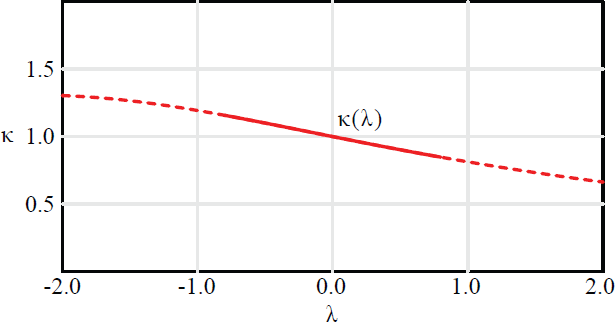
In the sequel, we denote E_app(λ) and µ_app(λ) respectively the energy and the corresponding chemical potential, with approximation up to order n = 6. We present their graphics based on determining the solution κ(λ) of Eq. (4.6), which are unique for any λ ≥ 0 (even for λ < 0 if |λ| is not very large). Figure 1 shows the graphic of the function λ ↦ κ(λ).

Figure 1:
Graphic of κ(λ) for λ ∈ [−2, 2]. The solid line corresponds to Eq. (4.6) in the interval of convergence of (4.4).

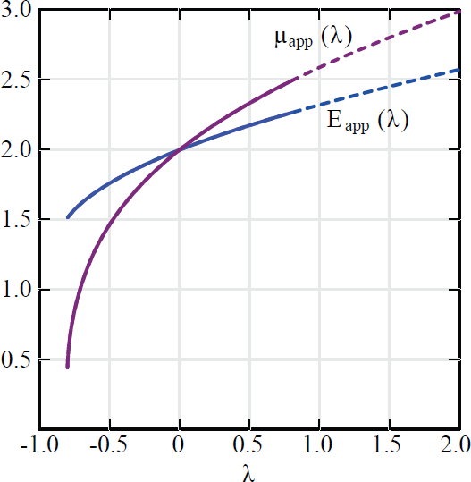
By using the values of κ(λ) in the Eq. (4.2) and numerical integration of the non-quadratic term with ψ_κ(λ), we obtain the graphics of E_app(λ) for λ ∈ (−λ_app, 2], where λ_app ≈ 0.78. Similarly, by using the values of E_app(λ) and numerical integration in Eq. (2.24), we obtain the graphic of µ_app(λ).

Figure 2:
Graphics of E _app(λ) (blue) and µ _app(λ) (purple) for λ ∈ (−λ _app , 2]. In both cases, the solid lines correspond to the interval of convergence of (4.4).

We can calculate the function κ(λ) by considering the implicity derivation of Eq. (4.6). More precisely,

$\frac{d}{d\lambda }f(\lambda ,\kappa (\lambda \left)\right)=\frac{\partial f}{\partial \lambda }+\frac{\partial f}{\partial \kappa }\frac{d\kappa }{d\lambda }=0,$ (4.8)

which allows us to determine the function κ(λ) as the solution to an initial value problem for ODEs, namely,

$\frac{d\kappa }{d\lambda }=-\frac{\partial f}{\partial \lambda }{\left(\frac{\partial f}{\partial \kappa }\right)}^{-1},\kappa \left(0\right)=1.$

This method produces similar results as before if λ is restrict to the interval of convergence of (4.4).

5 GENERALIZED THOMAS-FERMI APPROXIMATION

Under the condition that the kinetic energy be small enough, i.e. if

${\int }_{\mathrm{ℝ}}{\left|\phi \text{'}\left(s\right)\right|}^{2}ds\ll C_{\omega }{\int }_{\mathrm{ℝ}}{f}_{\lambda }\left(\phi \right(s\left)\right)\phi (s{)}^{2}ds,$

the term φ” is negligible, which means that, for λ > 0 large enough, the equation is reduced to

$f_{\lambda }\left(\phi \right(s\left)\right)=\frac{\mu -s^2}{C_{\omega }},$ (5.1)

where $f_{\lambda }\left(\rho \right)=\frac{3}{2}\sqrt{1+2\lambda {\rho }^2}-\frac{1}{2\sqrt{1+2\lambda {\rho }^2}}$.

It is clear that ρ ↦ f _λ (ρ) is strictly increasing in [0, +∞) and its inverse can be easily calculated. Indeed, from its definition we can write $f_{\lambda }\left(\rho \right):=h\left(\sqrt{1+2\lambda {\rho }^2}\right)$, where $\xi :=h\left(\eta \right)=\frac{1}{2}\left(3\eta -\frac{1}{\eta }\right)$, whose inverse is

$h^{-1}\left(\xi \right)=\frac{1}{3}\left(\xi +\sqrt{{\xi }^2+3}\right).$

Therefore, from (5.1) we get

$\sqrt{1+2\lambda \phi (s{)}^2}=h^{-1}\left(\frac{\mu -s^2}{C_{\omega }}\right)=\frac{\mu }{3C_{\omega }}\left(1-\frac{s^2}{\mu }+\sqrt{{\left(1-\frac{s^2}{\mu }\right)}^2+\frac{3C_{\omega }^2}{{\mu }^2}}\right),$

or equivalently,

$1+2\lambda \phi (s{)}^2=\frac{2{\mu }^2}{9C_{\omega }^2}\left[{\left(1-\frac{s^2}{\mu }\right)}^2+\left(1-\frac{s^2}{\mu }\right)\sqrt{{\left(1-\frac{s^2}{\mu }\right)}^2+\frac{3C_{\omega }^2}{{\mu }^2}}\right]+\frac{1}{3}.$

From the fact that µ is large if λ > 0 is large enough (see Lemma (3.4)), we can assume that $C_{\omega }^2/{\mu }^2$ is negligible to get the following (first) approximation

$1+2\lambda \phi (s{)}^2=\frac{4{\mu }^2}{9C_{\omega }^2}{\left(1-\frac{s^2}{\mu }\right)}^2+\frac{1}{3}.$ (5.2)

Hence, considering that ${\int }_{-\sqrt{\mu }}^{\sqrt{\mu }}{\phi }_{\lambda }(s{)}^{2}ds\approx 1$ (and remembering the symmetry of φ), we get

$\frac{4{\mu }^2\sqrt{\mu }}{9C_{\omega }^2}{\int }_0^1(1-u^2{)}^{2}du-\frac{2\sqrt{\mu }}{3}=\lambda .$ (5.3)

On the other hand, instead of simply discard the term 3C _ω /µ ², we can consider the approximation of $\sqrt{x+h}$ as $\sqrt{x}+h/2\sqrt{x}$, with x = (1 − s ² /µ)² and $h=3C_{\omega }^2/{\mu }^2$, to get

$1+2\lambda \phi (s{)}^2=\frac{4{\mu }^2}{9C_{\omega }^2}{\left(1-\frac{s^2}{\mu }\right)}^2+\frac{2}{3},$ (5.4)

which gives the (second) approximation

$\frac{4{\mu }^2\sqrt{\mu }}{9C_{\omega }^2}{\int }_0^1(1-u^2{)}^{2}du-\frac{\sqrt{\mu }}{3}=\lambda .$

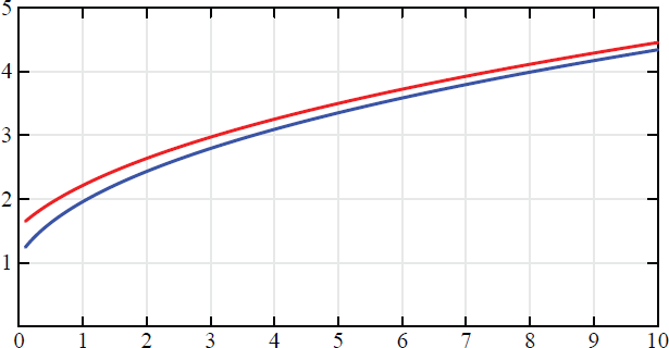
The solutions of (5.3) and (5.5) provide good approximations for µ as functions of λ - the generalized (first and second) Thomas-Fermi approximations -, as shown in Figure 3 (where we still have considered C _ω = 1 for numerical calculations).

Figure 3:
Graphics of µ(λ) for λ ∈ (0, 10] by Thomas-Fermi approximation. The red line corresponds to Eq. (5.3) and the blue one, to Eq. (5.5).

6 CONCLUSIONS

In this paper we present some important mathematical properties of the ground-state solutions of one-dimensional effective model proposed by A. Mun˜oz Mateo and V. Delgado to describe the cigar-shaped Bose-Einstein condensates in harmonic trap potentials. In Section 2, we prove, in the case of repulsive interatomic forces (λ > 0), that there exists a unique positive and symmetric ground state φ _min, decreasing for s > 0 (Theorems 2.2 and 2.3), which is orbitally stable in the Hilbert space of finite energy functions (Theorem 2.4). Moreover, like any other solution of Eq. (1.3), such ground state has a Gausssian-like exponential asymptotic decay (Theorem 2.1). In section 3 we describe the minimal energy E _min and the corresponding chemical potential µ _min as functions of the parameter λ , for which some general properties are shown (Lemma 3.4). All theses properties suggest that Gaussian functions could be used as approximations of those BECs. Based on this idea, we present in Section 4 some numerical examples. Finally, in Section 5, we describe an extension of the Thomas-Fermi approach to calculate the chemical potential in the context of large λ > 0.

Data availability

All data generated or analysed during this study are included in this published article.

REFERENCES

• ¹ M.H.J. Anderson, J.R. Ensher, M.R. Matthews & C.E. Wieman. Observation of Bose-Einstein condensation in a dilute atomic vapor. Science, 269(5221) (1995), 198-201.
• ² S. Bose. Plancks gesetz und lichtquantenhypothese. Zeitschrift für Physik, (26) (1924), 178-181.
• ³ R. Carles. Remarks on nonlinear Scherödinger equation with harmonic potential. Ann. Henri Poincaré, 3 (2002), 757-772.
• ⁴ R. Carretero-González, D.J. Frantzeskakis & P.G. Kevrekidis. Nonlinear waves in Bose-Einstein condensates: physical lelevance and mathematical techniques. Nonlinearity, 21 (2008), R139-R202.
• ⁵ T. Cazenave & P.L. Lions. Orbital stability of standing waves for some nonlinear Schrödinger equations. Comm. Math. Phys, 85 (1982), 549-561.
• ⁶ R. Cipolatti, Y.M. Lira & C. Trallero-Giner. Nonlinear Schrödinger equations with single power nonlinearity and harmonc potential. J. Phys. A: Math. Theor., 51 (2018), 115201-115218.
• ⁷ K..B.. Davis, M.O. Mewes, M.R. Andrews, N..J. van Druten, D.S. Durfee, D.M. Kurn & W. Ketterle. Bose-Einstein condensation in a gas of sodium atoms. Phys. Rev. Lett., (75) (1995), 27.
• ⁸ A. Einstein. Quantentheorie des einatomigen idealen Gases I. Sitzungsberichte der Preussischen Akademie der Wissenschaften (Proceedings of the Prussian Academy of Sciences), (21) (1924), 261-267.
• ⁹ A. Einstein. Quantentheorie des einatomigen idealen Gases, Zweite Abhandlung. Sitzungsberichte der Preussischen Akademie der Wissenschaften (Proceedings of the Prussian Academy of Sciences) , (3) (1925), 261.
• ¹⁰ A. Griffin, D.W. Snoke & S. Stringari. “Bose-Einstein Condensation”. Cambridge University Press (1995).
• ¹¹ E.P. Gross. Hydrodynamics of a superfluid condensate. Journal of Mathematical Physics, 4(2) (1963), 195-207.
• ¹² O. Kavian & F. Weissler. Self-similar solutions of the pseudo-conformally invariant nonlinear Schrödinger equation. Michigan Math. J., 41 (1994), 151-173.
• ¹³ E.H. Lieb & M. Loss. “Analysis”. Graduate Studies in Mathematics, Vol.14 (2nd Edition), AMS (2001).
• ¹⁴ E.H. Lieb, R. Seiringer & J. Yngvason. Bosons in a trap: a rigorous derivation of the Gross-Pitaevskii energy functional. Physical Review A, 61 (2000), 043602.
• ¹⁵ A.M. Mateo & V. Delgado. Effective one-dimensional dynamics of elongated Bosw-Winstein condensates. Annals of Physics, 324 (2009), 709.
• ¹⁶ A.M. Mateo & V. Delgado. Effective equation for matter-wave gap solitons in higher-order transversal states. Phys. Rev. E, 88 (2013), 042916.
• ¹⁷ J. Mossino. “Inegalités Isoperimetriques et Aplications en Physique”. Hermann (1984).
• ¹⁸ L.P. Pitaevskii. Vortex lines in an imperfect Bose gas. Soviet Physics JETP, 13(12) (1961), 451.
• ¹⁹ L. Salasnich, A. Parola & L. Reatto. Effective wave equation for the dynamics of cigar-shaped and disk-shaped Bose condensates. Phys. Rev. A, 043614 (2002), 65.
• ²⁰ C. Trallero-Giner, R. Cipolatti & T.C.H. Liew. One-dimensional cubic-quintic Gross-Pitaevskii equation for Bose-Einstein condensates in a trap potential. The European Physical Journal D, 67(143) (2013), 1-7.

Edited by

• Associate editor:
  Mustapha Rachidi

Publication Dates

• Publication in this collection
  27 July 2026
• Date of issue
  2026

History

• Received
  20 Jan 2026
• Accepted
  01 June 2026