Three-Dimensional Simulation of Neutron Flux Distribution in Boron Neutron Capture Therapy (BNCT)

ABSTRACT

Glioblastoma Multiforme (GBM) is one of the most aggressive and difficult-to-treat forms of malignant brain tumor, presenting a high incidence and resistance to conventional treatment methods. Boron Neutron Capture Therapy (BNCT) stands out as an innovative and promising approach for treating complex tumors such as GBM, as it enables the selective destruction of tumor cells with minimal impact on healthy tissues. In this study, the multigroup neutron diffusion equation is solved in a three-dimensional domain using four energy groups. The neutron source is represented as a boundary condition, and after diagonalizing the system of equations, the method of Separation of Variables can be applied to obtain an closed-form eigenfunction expansion. The validation of the proposed approach was carried out through numerical simulations in a water phantom, whose results indicated that thermal and epithermal neutron fluxes are predominant.

Keywords:
BNCT; neutron flux; neutron diffusion equation; closed-form eigenfunction expansion; method of separation of variables

1 INTRODUCTION

Glioblastoma multiforme (GBM) is the most common and aggressive type of brain tumor. Classified as a glioma, it originates from glial cells, which provide support and protection to neurons. GBM is characterized by rapid and invasive growth, making complete removal difficult and leading to a high recurrence rate. Despite advances in medicine and cancer therapies, the prognosis for patients diagnosed with GBM remains challenging, with a survival rate of only 5% five years after diagnosis.

The choice of treatment for GBM is individualized, considering the tumor’s location and extent, as well as the patient’s response. Surgical resection is often chosen to remove as much tumor tissue as possible without compromising essential neurological functions. However, due to the infiltrative nature of GBM, complete removal is rarely achieved, making the use of additional therapies necessary. Radiotherapy and chemotherapy are widely employed to slow tumor progression. Furthermore, emerging approaches such as immunotherapy ^{5), (9} and Boron Neutron Capture Therapy (BNCT) ^{2), (3), (4), (6), (7), (8), (13), (15} are being studied to enhance treatment efficacy and minimize damage to healthy tissues.

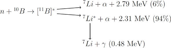
BNCT utilizes the nuclear reaction between a neutron and the boron-10 isotope (¹⁰B). This method is based on the administration of a compound containing ¹⁰B, which selectively accumulates in tumor tissue. After this concentration, the patient is irradiated with neutrons, triggering a nuclear reaction that releases alpha particles and lithium-7 (⁷ Li) nuclei, both with high linear energy transfer. The boron capture reaction is described as follows:

Figure 1:
Boron capture reaction.

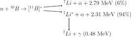
The main advantage of BNCT lies in its high specificity for cellular damage, as the emitted particles have a short range-approximately 9 micrometers for alpha particles and 5 micrometers for lithium nuclei, totaling only 14 micrometers ¹⁰. This range is smaller than the average cell diameter, ensuring that destruction occurs predominantly in tumor cells that have absorbed boron, while adjacent healthy cells are spared. Therefore, the precise determination of neutron and gamma dose rates is essential to ensure the safety and effectiveness of the treatment. Thus, BNCT represents a promising alternative for the treatment of tumors resistant to conventional therapies.

Historically, BNCT (Boron Neutron Capture Therapy) used nuclear reactors as a neutron source, as only these facilities could generate sufficiently intense thermal and epithermal neutron fluxes. Currently, there is a movement to replace reactors with accelerator-based neutron sources, which can be installed in hospitals, facilitating the spread of BNCT as a viable alternative in oncological treatment. Although few reactor-based facilities remain active (in Argentina, China, Japan, and Taiwan), these facilities continue to play a key role in advancing BNCT ¹. In Japan, since 2020, BNCT has been employed in the clinical treatment of inoperable head and neck carcinomas, using accelerator-based neutron sources. With the increasing number of patients undergoing this therapy, it has become essential to improve treatment planning systems to optimize the dose and maximize therapeutic efficacy ¹³.

Currently, Monte Carlo algorithms are the most commonly used methods for BNCT planning ^{2), (3), (4), (8), (13), (15}, but there is a growing demand for faster and equally accurate methods for dose calculation. Studies have explored new approaches to improve the efficiency of dose calculations in BNCT. For example, ¹⁵ calculated neutron flux distributions in a head and neck phantom using multigroup diffusion equations, reducing computation time compared to the Monte Carlo method, but with lower accuracy. ⁷ proposes a hybrid method for calculating neutron flux in BNCT, combining Monte Carlo simulations with diffusion equations using DIF3D (finite difference method).

In this work, we aim to solve the multigroup neutron diffusion equation in a three-dimensional domain, considering four energy groups, with the goal of analyzing the behavior of the neutron flux used in BNCT treatment. To achieve this, the neutron source is placed at the boundary at x = 0, transforming the problem into a homogeneous formulation. Furthermore, the system of equations is diagonalized, allowing the decoupling of the differential equations and their independent solution. The final solution is obtained using the method of Separation of Variables.

The physical environment considered consists of a homogeneous water phantom, commonly used as an approximation of soft biological tissue in BNCT studies, where the neutron beam is assumed to be incident perpendicularly at the boundary x = 0. The computational implementation is carried out in Python by numerically evaluating the closed-form eigenfunction expansion, truncated to a finite number of modes.

Unlike the works presented in the literature, the proposal of this study is to present a solution with lower computational time than the Monte Carlo Method and without the inherent approximations of numerical methods. Numerical simulations are presented on a water phantom, and the results obtained are consistent with those reported in the literature.

2 METHODOLOGY

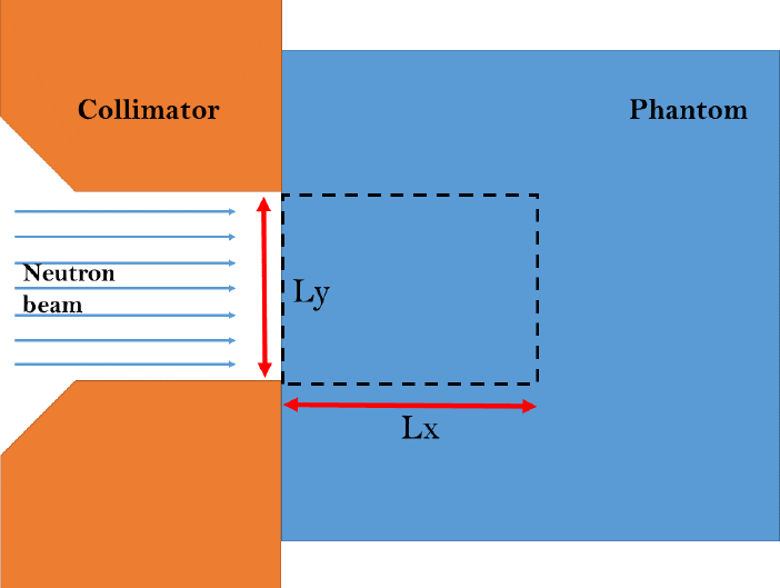
To model the neutron flux exiting a reactor or accelerator used in BNCT treatment, a phantom (a structure designed to simulate the physical and radiological properties of biological tissues) composed of water is considered to study the neutron distribution.

In Figure 2, a representative schematic of a cross-sectional view can be observed, where an orange structure represents the collimator of the irradiation system. The neutron beam (horizontal blue arrows) exits the collimator and enters the region of interest. These neutrons are directed to enter perpendicularly on the water phantom. Inside the phantom, there is a black dashed rectangle, indicating a region of interest where the neutron flux distribution will be analyzed.

Figure 2:
Cross-sectional view of the water phantom.

To model this process, the following equation is a form of the stationary multigroup diffusion equation for neutrons, used to describe the distribution of neutron flux considering their interactions with the medium ^{11), (12}:

$-D_g{\nabla }^2{\Phi }_g+{\Sigma }_{R,g}{\Phi }_g=\sum _{g\text{'}-1}^{g-1}{\Sigma }_{s,g\text{'}\to g}{\Phi }_{g\text{'}}+S_g,$

where Φ_g is the neutron flux in group g, D _g is the diffusion coefficient, Σ_R,g is the macroscopic removal cross section, Σ_s,g’→g is the macroscopic scattering cross section, and S _g is an external neutron source. The macroscopic cross sections and diffusion coefficients adopted in this work are obtained from the removal-diffusion framework reported in ^{11), (12}, which provides representative group constants commonly used in BNCT modeling.

The approach proposed in this work consists of reformulating the neutron diffusion equation by treating the source as a boundary condition at x = 0. This strategy allows the application of the method of separation of variables, leading to a closed-form eigenfunction expansion of the problem.

$-D_g{\nabla }^2{\Phi }_g+{\Sigma }_{R,g}{\Phi }_g=\sum _{g\text{'}-1}^{g-1}{\Sigma }_{s,g\text{'}\to g}{\Phi }_{g\text{'}}.$ (2.1)

When applying this formulation to a domain representing a region of brain tissue with a well-defined geometry, homogeneous Dirichlet boundary conditions are imposed, i.e., Φ_g = 0 on the domain boundaries. This assumption corresponds to an idealized absorbing boundary and ensures that no particles remain within the system beyond the prescribed limits, which is consistent with the mathematical formulation adopted. In particular, such a choice allows the use of separation of variables and eigenfunction expansion, enabling the derivation of closed-form modal solutions with reduced computational cost.

At the entrance boundary x = 0, a non-homogeneous condition is prescribed in the form Φ_g (0, y, z) = f, representing the incident neutron beam. In this formulation, the function f is obtained by evaluating the source term at x = 0, ensuring consistency between the mathematical model and the imposed driving condition.

It is important to note that, from a physical standpoint, homogeneous Dirichlet conditions may represent an idealized absorbing boundary and do not fully capture realistic neutron behavior at the domain limits, where more accurate treatments typically involve vacuum conditions, extrapolated boundary distances, or albedo-type formulations. Similarly, prescribing the flux at the entrance boundary constitutes a simplified representation of the incident beam, which in a more rigorous framework would be described in terms of incoming neutron current or mixed (Robin-type) boundary conditions. Nevertheless, such simplified boundary assumptions are commonly adopted in analytical and semi-analytical models aimed at capturing the dominant features of the neutron flux distribution while preserving mathematical tractability. In particular, this approach is consistent with reaction-diffusion models used in the mathematical modeling of tumor growth, such as those proposed by ¹⁴, which rely on idealized domain conditions to maintain analytical structure. In the present work, this choice is further motivated by the perspective of coupling the neutron diffusion model with tumor evolution models of the Swanson type, ensuring compatibility within a unified modeling framework.

For the application of the methodology, the Equation (2.1) is first rewritten in matrix form:

$-\mathit{D}{\nabla }^2\mathit{\Phi }+\mathit{\Sigma }\mathit{\Phi }=\overline{0},$ (2.2)

where:

$$\begin{gathered} \mathit{D}=\left[\begin{array}{cccc}{D}_1& 0& 0& 0\\ 0& D_2& 0& 0\\ 0& 0& D_3& 0\\ 0& 0& 0& D_4\end{array}\right], \\ \Sigma =\left[\begin{array}{cccc}{\Sigma }_{R,1}& 0& 0& 0\\ -{\Sigma }_{s,1\to 2}& {\Sigma }_{R,2}& 0& 0\\ -{\Sigma }_{s,1\to 3}& -{\Sigma }_{s,2\to 3}& {\Sigma }_{R,3}& 0\\ -{\Sigma }_{s,1\to 4}& -{\Sigma }_{s,2\to 4}& -{\Sigma }_{s,3\to 4}& {\Sigma }_{R,4}\end{array}\right], \end{gathered}$$

∇2Φ denotes the application of the Laplacian operator to the neutron flux vector Φ, and $\overline{0}$ is a null vector.

To decouple the system of equations and solve them independently, Σ is diagonalized. For this, a matrix P is used such that P ⁻¹ ΣP = Λ, where Λ is a diagonal matrix whose elements are the eigenvalues λ _i of the matrix Σ, and P is composed of the eigenvectors of Σ. Since Σ is a lower triangular matrix, its eigenvalues are simply the entries on its main diagonal:

$\mathit{\Lambda }=\left[\begin{array}{cccc}{\lambda }_1& 0& 0& 0\\ 0& {\lambda }_2& 0& 0\\ 0& 0& {\lambda }_3& 0\\ 0& 0& 0& {\lambda }_4\end{array}\right]=\left[\begin{array}{cccc}{\Sigma }_{R,1}& 0& 0& 0\\ 0& {\Sigma }_{R,2}& 0& 0\\ 0& 0& {\Sigma }_{R,3}& 0\\ 0& 0& 0& \Sigma R,4\end{array}\right].$

Thus, a new unknown vector is defined as Ψ = P ⁻¹ Φ, and Φ = PΨ is substituted into Equation (2.2), yielding:

$-\mathit{D}{\mathbf{\nabla }}^2\mathit{\Psi }+\mathit{\Lambda }\mathit{\Psi }=\overline{0},$

which results in a system of four decoupled partial differential equations:

$$\begin{gathered} -D_1{\nabla }^2{\Psi }_1+{\lambda }_1{\Psi }_1=0, \\ -D_2{\nabla }^2{\Psi }_2+{\lambda }_2{\Psi }_2=0, \\ -D_3{\nabla }^2{\Psi }_3+{\lambda }_3{\Psi }_3=0, \\ -D_4{\nabla }^2{\Psi }_4+{\lambda }_4{\Psi }_4=0, \end{gathered}$$

Now, the decoupled partial differential equations can be solved for each energy group by applying the method of Separation of Variables:

${\Psi }_g\left(x,y,z\right)=X\left(x\right)Y\left(y\right)Z\left(z\right).$

Substituting the separated solution ${\Psi }_g\left(x,y,z\right)=X\left(x\right)Y\left(y\right)Z\left(z\right).$ into the decoupled partial differential equation, we obtain:

$-D_g{\nabla }^2\left[X\left(x\right)Y\left(y\right)Z\left(z\right)\right]+{\lambda }_{i}X\left(x\right)Y\left(y\right)Z\left(z\right)=0.$

Expanding the Laplacian operator, it follows that:

$Y\left(y\right)Z\left(z\right)\frac{d^{2}X\left(x\right)}{d{x}^2}+X\left(x\right)Z\left(z\right)\frac{d^{2}Y\left(y\right)}{d{y}^2}+X\left(x\right)Y\left(y\right)\frac{d^{2}Z\left(z\right)}{d{z}^2}-\frac{{\lambda }_i}{D_g}X\left(x\right)Y\left(y\right)Z\left(z\right)=0.$

Dividing both sides by X(x)Y(y)Z(z), we obtain:

$\frac{1}{X\left(x\right)}\frac{d^{2}X\left(x\right)}{d{x}^2}+\frac{1}{Y\left(y\right)}\frac{d^{2}Y\left(y\right)}{d{y}^2}+\frac{1}{Z\left(z\right)}\frac{dZ\left(z\right)}{d{z}^2}=\frac{{\lambda }_i}{D_g}.$

Defining ${\gamma }_g=\frac{{\lambda }_i}{D_g}$ and introducing a separation constant σ ₁, we assume:

$\frac{1}{Z\left(z\right)}\frac{d^{2}Z\left(z\right)}{d{z}^2}={\sigma }_1.$

Substituting into the previous equation yields:

$\frac{1}{X\left(x\right)}\frac{d^{2}X\left(x\right)}{d{x}^2}+\frac{1}{Y\left(y\right)}\frac{d^{2}Y\left(y\right)}{d{y}^2}+{\sigma }_1={\gamma }_g.$

Rearranging terms and introducing a second separation constant σ ₂, we obtain:

$\frac{1}{X\left(x\right)}\frac{d^{2}X\left(x\right)}{d{x}^2}+\left({\sigma }_1-{\gamma }_g\right)=-\frac{1}{Y\left(y\right)}\frac{d^{2}Y\left(y\right)}{d{y}^2}={\sigma }_2.$

Thus, we arrive at the following system of ordinary differential equations:

$$\begin{gathered} \frac{d^{2}X\left(x\right)}{d{x}^2}+\left({\sigma }_1-{\gamma }_g-{\sigma }_2\right)X\left(x\right)=0, \\ \frac{d^{2}Y\left(y\right)}{d{y}^2}+{\sigma }_{2}Y\left(y\right)=0, \\ \frac{d^{2}Z\left(z\right)}{d{z}^2}+{\sigma }_{1}Z\left(z\right)=0. \end{gathered}$$

This system of ordinary differential equations has well-known analytical solutions in the literature, with ${\sigma }_2={\xi }_2^2>0$ and ${\sigma }_1={\xi }_1^2<0$.

By combining the solutions of these ordinary differential equations, the general solution can be obtained as the product of the individual solutions. Thus, the solution for Ψ_g is:

${\Psi }_g=\sum _{m=1}^{\infty }\sum _{l=1}^{\infty }{A}_{l,m}\left[-e^{2{\xi }_{3,l,m^{L_x}}}{e}^{{\xi }_{3,l,m^x}}+e^{-{\xi }_{3,l,m^x}}\right]\sin \left({\xi }_{2,m}y\right)\sin \left({\xi }_{1,l}z\right),$

where ${\xi }_{1,l}=\frac{l\mathrm{\pi }}{L_z}$, with l = 1, 2, . . .; ${\xi }_{2,m}=\frac{m\mathrm{\pi }}{L_y}$, with m = 1, 2, . . .; and ${\xi }_{3,l,m}=\sqrt{{\gamma }_g+{\xi }_{2,m}^2+{\xi }_{1,l}^2}$.

To explicitly determine the coefficients A _l,m , we apply the non-homogeneous boundary condition at x = 0. Substituting into the general solution, we obtain:

$P^{-1}f=\sum _{m=1}^{\infty }\sum _{l=1}^{\infty }{A}_{l,m}\left[-e^{2{\xi }_{3,l,m}{L}_x}+1\right]\sin \left({\xi }_{2,m}y\right)\sin \left({\xi }_{1,lz}\right).$

Using the orthogonality properties of the sine eigenfunctions, the coefficients A _l,m can be determined as:

$A_{l,m}=\frac{{\int }_0^{L_y}{\int }_0^{L_z}{\mathit{P}}^{-1}f\sin \left({\xi }_{2,m}y\right)\sin \left({\xi }_{1,l}z\right)dzdy}{\left[-e^{-2{\xi }_{3,l,m}{L}_x}+1\right]{\int }_0^{L_y}{\sin }^2\left({\xi }_{2,m}y\right)dy{\int }_0^{L_z}{\sin }^2\left({\xi }_{1,l}z\right)dz}.$

Finally, it is sufficient to revert to the original variable Φ = PΨ to obtain the final solution of the problem.

To improve the clarity and reproducibility of the computational procedure, a flowchart summarizing the main steps of the methodology is presented in Figure 3. The diagram outlines the sequence of operations, including the definition of the physical and numerical parameters, the formulation and diagonalization of the multigroup system, the application of the separation of variables technique, and the reconstruction of the neutron flux. This representation provides a structured overview of the implementation adopted in this work.

Figure 3:
Flowchart of the computational procedure adopted to solve the three-dimensional multi-group neutron diffusion equation.

2.1 Analytical Residual of the Truncated Modal Expansion

To complement the convergence analysis based on the relative change in the neutron flux between successive truncation levels, an additional consistency verification can be carried out through the residual of the governing multigroup diffusion equations. Since the solution proposed in this work is obtained in analytical form as a closed-form eigenfunction expansion, it is more appropriate to evaluate the residual using the analytical structure of the truncated series itself. This choice ensures that the residual reflects only the effects of modal truncation and floating-point arithmetic, and not additional discretization errors.

After diagonalization of the multigroup system, the governing equations are decoupled and written, for each energy group g, as

$-D_g{\nabla }^2{\Psi }_g+{\lambda }_i{\Psi }_g=0,$

The truncated solution for each group is expressed as

${\Psi }_g^{\left(L,M\right)}\left(x,y,z\right)=\sum _{m=1}^M\sum _{l=1}^L{A}_{l,m}^{\left(g\right)}\left[-e^{-2{\xi }_{3,l,m}^{\left(g\right)}{L}_x}{e}^{{\xi }_{3,l,m}^{\left(g\right)}x}+e^{-{\xi }_{3,l,m}^{\left(g\right)}x}\right]\sin \left({\xi }_{2,m}y\right)\sin \left({\xi }_{1,l}z\right),$

where L and M denote the truncation levels in the modal indices.

To evaluate the analytical residual, it is useful to observe that each retained modal term satisfies the decoupled differential operator analytically. Indeed, the second derivative of the exponential factor with respect to x yields

$\frac{{\partial }^2}{\partial x^2}\left[-e^{-2{\xi }_{3,l,m}^{\left(g\right)}{L}_x}{e}^{{\xi }_{3,l,m}^{\left(g\right)}x}+e^{{\xi }_{3,l,m}^{\left(g\right)}x}\right]={\left({\xi }_{3,lm}^{\left(g\right)}\right)}^2\left[-e^{-2{\xi }_{3,l,m}^{\left(g\right)}{L}_x}{e}^{{\xi }_{3,l,m}^{\left(g\right)}x}+e^{{\xi }_{3,l,m}^{\left(g\right)}x}\right].$

Similarly, the second derivatives of the trigonometric factors are

$$\begin{gathered} \frac{{\partial }^2}{\partial y^2}\sin \left({\xi }_{2,m}y\right)=-{\xi }_{2,m}^2\sin \left({\xi }_{2,m}y\right), \\ \frac{{\partial }^2}{\partial z^2}\sin \left({\xi }_{1,l}z\right)=-{\xi }_{1,l}^2\sin \left({\xi }_{1,l}z\right). \end{gathered}$$

Therefore, for each modal contribution, the Laplacian operator produces the factor

${\left({\xi }_{3,l,m}^{\left(g\right)}\right)}^2-{\xi }_{2,m}^2-{\xi }_{1,l}^2.$

Using the definition of ${\xi }_{3,l,m}^{\left(g\right)}$, it follows immediately that

${\left({\xi }_{3,l,m}^{\left(g\right)}\right)}^2-{\xi }_{2,m}^2-{\xi }_{1,l}^2={\gamma }_g.$

Hence, the Laplacian of the truncated solution satisfies

${\nabla }^2{\Psi }_g^{\left(L,M\right)}={\gamma }_g{\Psi }_g^{\left(L,M\right)}.$

Substituting this relation into the decoupled equation, the analytical residual associated with the truncated expansion can be written as

$R_{\Psi ,g}^{\left(L,M\right)}\left(x,y,z\right)=-D_g{\nabla }^2{\Psi }_g^{\left(L,M\right)}\left(x,y,z\right)+{\lambda }_i{\Psi }_g^{\left(L,M\right)}\left(x,y,z\right),$

which, using the previous identity, becomes

$R_{\Psi ,g}^{\left(L,M\right)}\left(x,y,z\right)=-\left(D_g{\gamma }_g+{\lambda }_i\right){\Psi }_g^{\left(L,M\right)}\left(x,y,z\right).$ (2.3)

Since γ _g = λ _i /D _g , the coefficient in parentheses is theoretically zero, and therefore

$R_{\Psi ,g}^{\left(L,M\right)}\left(x,y,z\right)=0$

for the exact analytical representation. In practical numerical implementation, however, a very small nonzero residual may appear due to floating-point round-off and the numerical diagonalization of the matrix Σ.

To quantify this effect, the relative residual is evaluated by means of the L ² norm over the spatial domain Ω:

${\tilde{\epsilon }}_{R_g}^{\left(L,M\right)}=\frac{{||R_{\Psi ,g}^{\left(L,M\right)}||}_{L^2\left(\Omega \right)}}{{||{\Psi }_g^{\left(L,M\right)}||}_{L^2\left(\Omega \right)}},g=1,...,G.$

A global residual indicator may also be defined as

${\tilde{\epsilon }}_R^{\left(L,M\right)}=\frac{{\left(\sum _{g=1}^G{||R_{\Psi ,g}^{\left(L,M\right)}||}_{L^2\left(\Omega \right)}^2\right)}^{1/2}}{{\left(\sum _{g=1}^G{||{\Psi }_g^{\left(L,M\right)}||}_{L^2\left(\Omega \right)}^2\right)}^{1/2}}.$

It is important to emphasize that this residual does not measure the convergence of the modal truncation itself, since each retained mode already satisfies the decoupled differential equation analytically. Instead, the analytical residual serves as a consistency check of the implementation. For this reason, the convergence of the truncated expansion is more informatively assessed through the relative change in the flux between successive truncation levels, while the analytical residual verifies that the truncated modal representation remains fully consistent with the governing operator up to machine precision. Let Φ ^(L,M) denote the multigroup flux obtained with truncation levels L and M. The relative variation is given by

${\epsilon }_{\Phi }^{\left(L,M\right)}=\frac{{||{\Phi }^{\left(L,M\right)}-{\Phi }^{\left(L-1,M-1\right)}||}_{L^2\left(\Omega \right)}}{{||{\Phi }^{\left(L,M\right)}||}_{L^2\left(\Omega \right)}},$ (2.4)

where ${||·||}_{L^2\left(\Omega \right)}$ denotes the L ² norm over the spatial domain Ω, defined as

${||{\mathit{\Phi }}^{\left(L,M\right)}||}_{L^2\left(\Omega \right)}={\left(\sum _{g=1}^G{\int }_{\Omega }{\left|{\Phi }_g^{\left(L,M\right)}\left(x,y,z\right)\right|}^{2}d\Omega \right)}^{1/2}.$

Since the spectral behavior is particularly relevant in BNCT applications, this indicator can also be evaluated separately for each energy group:

${\epsilon }_{{\Phi }_g}^{\left(L,M\right)}=\frac{{||{\Phi }_g^{\left(L,M\right)}-{\Phi }_g^{\left(L-1,M-1\right)}||}_{L^2\left(\Omega \right)}}{{||{\Phi }_g^{\left(L,M\right)}||}_{L^2\left(\Omega \right)}},g=1,...,G.$

The truncation levels can be selected such that the relative flux variation satisfy prescribed tolerance, i.e.,

${\epsilon }_{{\Phi }_g}^{\left(L,M\right)}<to{l}_{\Phi }\text{and}{\tilde{\epsilon }}_{R_g}^{\left(L,M\right)}<to{l}_R,$

ensuring that the truncated solution provides an accurate and converged semi-analytical approximation of the multigroup neutron flux.

2.2 Results and Discussions

The numerical simulation of the solution found to determine the behavior of the neutron flux was performed in Python. Four energy groups were used, where Group 1 covers energies between 1.0 × 10³ and 3.0 × 10⁵ eV, Group 2 includes neutrons with energies ranging from 10 to 1.0 × 10³ eV, Group 3 encompasses neutrons with energies between 0.4 and 10 eV, while Group 4 has an energy range from 0 to 0.4 eV. For the energy group intensities related to the non-homogeneous boundary condition, an approximation was used where a function is inversely proportional to the mean energy range of each group ^{11), (12}.

The physical environment consists of a homogeneous water phantom, commonly used to approximate soft biological tissue in BNCT studies. The domain considered for the simulation has dimensions L _x = 5.0, L _y = 3.0, and L _z = 3.0. The computational implementation was carried out in Python, using a structured grid with spatial discretization ∆x = ∆y = ∆z = 0.01. The closed-form eigenfunction expansion was evaluated by truncating the modal indices to L = M = 25, retaining a finite number of modes in each spatial direction. The numerical evaluation and visualization of the results were performed using standard scientific computing libraries.

The neutron beam is assumed to be incident perpendicularly at the boundary x = 0. The medium is considered homogeneous, and no heterogeneities are included in the present model.

The macroscopic cross sections and diffusion coefficients employed in this study were obtained from the literature, specifically from the removal-diffusion framework presented in ^{11), (12} (Table 1). These parameters are representative of typical materials used in BNCT modeling and are widely adopted in studies involving neutron transport in biological media.

Table 1:
Parameters used in the numerical simulation. Source: Adapted from ^{11), (12}.

g	Dg [cm]	ΣR,g [1/cm]	Σs,g′−g [1/cm]	Σs,g′−g [1/cm]
			(g-1→g)	(g-2→g)
1	2.0 × 10−1	1.572 × 10−1	-	-
2	2.5 × 10−1	1.1 × 10−1	6 × 10−2	-
3	2.2 × 10−1	9.7 × 10−2	6.1 × 10−2	-
4	2.1 × 10−2	2.2 × 10−3	0	5.228 × 10−2

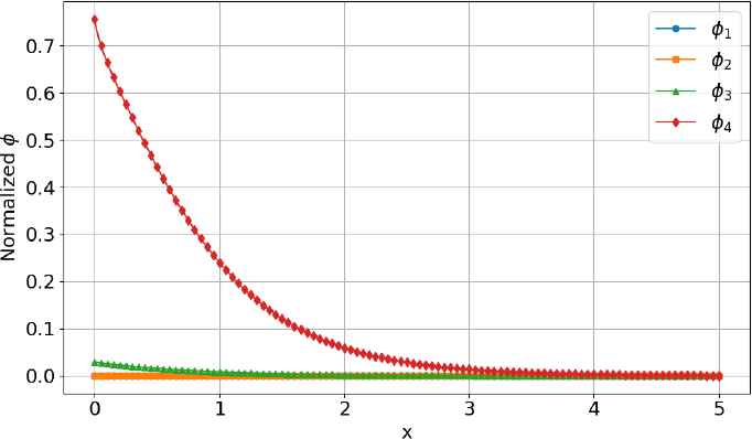
Figure 4 illustrates the distribution of fluxes as a function of depth x in the phantom, at the center of the mesh of y and z. It can be observed that the neutron fluxes decrease exponentially as the depth increases. It is also noted that the thermal and epithermal fluxes are more significant, which is in line with expectations for BNCT therapy, while the high-energy fluxes are nearly insignificant (close to zero).

Figure 4:
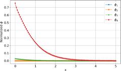
Flux distribution as a function of depth x in the phantom, in the middle of the y and z grid.

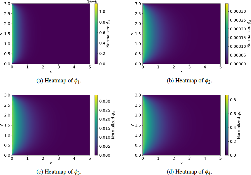
The Figure 5 shows the heatmaps of ϕ ₁, ϕ ₂, ϕ ₃, and ϕ ₄, respectively, in the plane at the midpoint of the mesh in the z-direction. It can be observed that the fluxes ϕ ₁ and ϕ ₂ tend to zero at the initial positions. The fluxes ϕ ₃ and ϕ ₄ decrease more gradually, as they lose energy progressively while interacting with the atoms of the medium (moderation effect).

Figure 5:
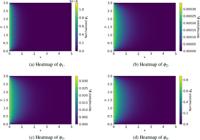
Heat maps of the variables ϕ ₁, ϕ ₂, ϕ ₃, and ϕ ₄ in the plane at the midpoint of the mesh in the z-direction.

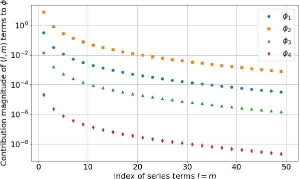
To further analyze the structure of the closed-form eigenfunction expansion obtained through the method of separation of variables, Figure 6 shows the magnitude of the modal coefficients corresponding to the indices (l, m) for each energy group. These coefficients determine the weight of each harmonic component in the reconstruction of the neutron flux and therefore indicate how rapidly the truncated series converges in practice.

Figure 6:
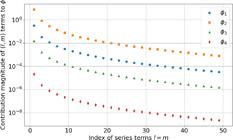
Contribution of the series terms (l, m) to the solution ϕ _g for each energy group, evaluated at the point (x, y, z) = (0.2, 1.5, 1.5).

As expected for diffusion-type problems with homogeneous boundary conditions, the contributions decrease monotonically as the indices l and m increase, revealing that the lowest-order harmonics dominate the spatial behavior of the flux. The analysis was carried out at the spatial point (x, y, z) = (0.2, 1.5, 1.5), corresponding to the mesh indices (i, j, k) = (2, ny/2, nz/2), which lies at the center of the domain in the y- and z-directions and near the boundary at x = 0, where the neutron source is applied. It was observed that the modal amplitudes decay rapidly, and for L = M = 30, the contribution of additional terms is of the order of 10⁻⁸ for the thermal group flux, indicating that the truncated solution provides an accurate approximation of the infinite series representation.

The results indicate that only a relatively small number of terms is required to accurately represent the solution, supporting the truncation strategy used in the numerical simulations. A practical stopping criterion can therefore be defined based on the magnitude of the incremental contribution of additional modes, ensuring that the relative change in the flux norm remains below a prescribed tolerance.

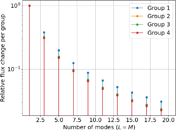
Using the formula (2.4), the truncation levels were taken as L = M, and the error was evaluated for increasing values of L = 1, 2, . . . , 20. The spatial norm was computed over the entire computational domain Ω. Additionally, for visualization purposes, modal contributions were also evaluated at a representative point located at (x, y, z) = (0.2, 1.5, 1.5), corresponding to a position near the beam entrance and centered in the transverse directions. Figure 7 presents the relative flux change for each energy group as a function of the number of retained modes.

Figure 7:
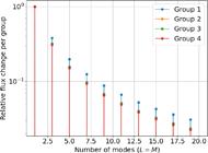
Convergence of the truncated modal expansion for each energy group, evaluated through the relative change in the neutron flux between successive truncation levels (L = M).

The results show a clear and monotonic decay of the error for all energy groups as the truncation level increases. In logarithmic scale, the curves exhibit an approximately linear behavior, indicating an exponential convergence of the modal expansion. This behavior is characteristic of solutions obtained through separation of variables and eigenfunction expansions.

It is also observed that the magnitude of the error differs slightly between energy groups. The higher-energy groups exhibit larger errors for a given truncation level, while the lower-energy (thermal) group converges more rapidly. This behavior is consistent with the smoother spatial distribution typically associated with thermal neutron fluxes, which are easier to represent with a limited number of modes. For truncation levels around L = M = 20, the relative change in the flux is already significantly reduced for all groups, indicating that additional modes contribute negligibly to the solution. This confirms that the adopted truncation level provides a stable and accurate approximation of the infinite-series representation.

Using the analytical structure of the expansion of the eigenfunction, the residual (Equation (2.3)) was calculated without introducing additional numerical discretization errors. As expected, the residual remains at the level of numerical round-off, confirming that each retained mode satisfies the differential operator consistently.

Overall, these results demonstrate that the proposed semi-analytical solution exhibits fast and robust convergence, and that the truncation strategy based on a finite number of modes is sufficient to accurately capture the multigroup neutron flux distribution.

3 FINAL CONSIDERATIONS

In this work, the solution to the multigroup neutron diffusion equation in a three-dimensional domain was presented, considering four energy groups. The behavior of the neutron flux employed in BNCT therapy for the treatment of GBM was studied. The approach used treats the neutron source, characteristic of the BNCT treatment, as a boundary condition at x = 0, homogenizing the problem and allowing the application of the method of Separation of Variables. Moreover, the system of equations was diagonalized, enabling the decoupling of the differential equations and their solution independently. It is worth noting that this study provides a closed-form eigenfunction expansion of the solution, avoiding spatial discretization errors typical of fully numerical methods, while maintaining reduced computational cost.

Although the solution is expressed in analytical form as a closed-form eigenfunction expansion, it consists of an infinite series which, in practice, must be truncated to a finite number of terms, resulting in a semi-analytical approximation. This truncation introduces a small approximation error, and the computational effort required depends on the number of terms considered in the series. An analysis of the contribution of the series terms was performed, showing that the higher-order terms rapidly decrease in magnitude, indicating fast convergence of the solution and justifying the truncation adopted in the numerical simulations. A convergence analysis was performed by evaluating both the relative change in the neutron flux and the normalized residual of the governing equations as a function of the truncation level. The results demonstrate a rapid decay of both error indicators, confirming that the adopted truncation level provides an accurate and stable approximation of the solution. The simulated results are in accordance with the dynamics of the problem.

As a perspective for future work, a systematic validation of the proposed method will be carried out through comparisons with results available in the literature. This will allow a detailed assessment of the accuracy of the multigroup flux predictions across different energy groups and spatial regions. It is important to emphasize that the primary objective of the present work was the development of a closed-form semi-analytical solution for the multigroup neutron diffusion equation, and therefore the focus was placed on the mathematical formulation and its properties.

Additionally, the present model can be extended to incorporate more physically realistic boundary conditions, such as vacuum, albedo, or mixed (Robin-type) formulations, allowing a more accurate representation of neutron leakage and incident beam characteristics. Furthermore, na important research direction consists in coupling the neutron diffusion model with reaction-diffusion models describing tumor cell dynamics, such as those proposed by ¹⁴. In this context, the computation of BNCT dose components based on the multigroup neutron flux will be incorporated, enabling a consistent link between neutron transport, dose deposition, and tumor response. This integrated approach may provide a unified framework for simulating both neutron flux and tumor evolution in BNCT, enabling more realistic and clinically relevant treatment modeling.

Data availability

Datasets related to this article are available upon request to the corresponding author.

Acknowledgments

The authors would like to thank FAPERGS (Fundação de Amparo à pesquisa do Estado do Rio Grande do Sul) for their financial support.

REFERENCES

• ¹ S. Altieri & N. Protti. A brief review on reactor-based neutron sources for boron neutron capture therapy. Therapeutic Radiology and Oncology, 2 (2018), 1-8. doi: 10.21037/tro.2018.10.08.
  » https://doi.org/10.21037/tro.2018.10.08
• ² F. Arianto, L.T. Handayani, W.S. Budi & P. Basuki. Determination of Neutron Flux in Brain Cancer Boron Neutron Capture Therapy Using Monte Carlo Simulation. Physics Communication, 6 (2022), 79-84. doi: 10.1016/j.nima.2022.167240.
  » https://doi.org/10.1016/j.nima.2022.167240
• ³ R.V. Balle. In Vivo Total Dose Analysis in Mice for BNCT Trial TRIGA Kartini Research Reactor Based Using PHITS. Indonesian Journal of Physics and Nuclear Applications, 4 (2019), 27-32. doi: 10.24246/ijpna.v4i1.27-32.
  » https://doi.org/10.24246/ijpna.v4i1.27-32
• ⁴ A.H. Bilalodin & F. Abdullatif. Dose analysis of Boron Neutron Capture Therapy (BNCT) on head cancer using PHITS code with neutron source from accelerator. Journal of Physics: Conference Series, 2498 (2023), 1-7. doi: 10.1088/1742-6596/2498/1/012044.
  » https://doi.org/10.1088/1742-6596/2498/1/012044
• ⁵ N.K. et al. Current state and future prospects of immunotherapy for glioma. Immunotherapy, 10 (2018), 317-339. doi: 10.2217/imt-2017-0122.
  » https://doi.org/10.2217/imt-2017-0122
• ⁶ IAEA. “Advances in Boron Neutron Capture Therapy”. International Atomic Energy Agency, Vienna (2023).
• ⁷ C. Lee, N. Jung & H. Lee. Neutron Flux Calculation for BNCT with Monte Carlo-Diffusion Hybrid Method. In “Transactions of the Korean Nuclear Society Virtual Autumn Meeting” (2020), p. 1-4.
• ⁸ G. Li, W. Jiang, L. Zhang, W. Chen & Q. Li. Design of Beam Shaping Assemblies for Accelerator-Based BNCT With Multi-Terminals. Frontiers in Public Health, 9 (2021), 642561. doi: 10.3389/fpubh.2021.642561.
  » https://doi.org/10.3389/fpubh.2021.642561
• ⁹ M. Lim, Y. Xia, C. Bettegowda & M. Weller. Current state of immunotherapy for glioblastoma. Nature Reviews Clinical Oncology, 15 (2018), 422-442. doi: 10.1038/s41571-018-0003-5.
  » https://doi.org/10.1038/s41571-018-0003-5
• ¹⁰ Y. Mishima, M. Ichihashi, S. Hatta, C. Honda, K. Yamamura & T. Nakagawa. New thermal neutron capture therapy for malignant melanoma: melanogenesis-seeking 10B molecule-melanoma cell interaction from in vitro to first clinical trial. Pigment Cell Research, 2(4) (1989), 226-234. doi: 10.1111/j.1600-0749.1989.tb00196.x.
  » https://doi.org/10.1111/j.1600-0749.1989.tb00196.x
• ¹¹ J. Niemkiewicz & T.E. Blue. “Removal-Diffusion Theory for Calculation of Neutron Distributions in BNCT”. Springer US, Boston, MA (1993), p. 177-180. doi: 10.1007/978-1-4615-2978-135.
  » https://doi.org/10.1007/978-1-4615-2978-135
• ¹² J. Niemkiewicz, T.E. Blue & N. Gupta. Calculation of neutron flux distributions in BNCT using removal-diffusion theory. Transactions of the American Nuclear Society, 70 (1994).
• ¹³ M. Nojiri, T. Takata, N. Hu, Y. Sakurai, M. Suzuki & H. Tanaka. Neutron flux evaluation algorithm with a combination of Monte Carlo and removal-diffusion calculation methods for boron neutron capture therapy. Medical Physics, 51(5) (2024), 3711-3724. doi: 10.1002/mp.16931.
  » https://doi.org/10.1002/mp.16931
• ¹⁴ R. Rockne, E.C. Alvord Jr., J.K. Rockhill & K.R. Swanson. A mathematical model for brain tumor response to radiation therapy. Journal of Mathematical Biology, 58(4-5) (2009), 561-578. doi: 10.1007/s00285-008-0219-6.
  » https://doi.org/10.1007/s00285-008-0219-6
• ¹⁵ K. Takada, H. Kumada, P.H. Liem, H. Sakurai & T. Sakae. Development of Monte Carlo based real-time treatment planning system with fast calculation algorithm for boron neutron capture therapy. Physica Medica, 32(12) (2016), 1846-1851. doi: 10.1016/j.ejmp.2016.11.007.
  » https://doi.org/10.1016/j.ejmp.2016.11.007

Edited by

• Associate editor:
  Mustapha Rachidi

Publication Dates

• Publication in this collection
  20 July 2026
• Date of issue
  2026

History

• Received
  12 Dec 2025
• Accepted
  13 Apr 2026