A Simplified Kinetic Model for the Tropospheric Ozone Cycle

ABSTRACT

To better understand the dynamics of air pollutants, several mathematical or computational models have been developed and employed. Among the pollutants of interest are those related to the cycle of formation of tropospheric ozone (O₃), which involve nitrogen oxides NO_x. In this process, there is a sequence of chemical reactions whose most elementary modeling can be described in terms of ordinary differential equations (ODEs), in which the concentrations (in µg/m³) of gases (O, NO, NO₂, and O₃) are functions of time. A novel study of the model is presented in terms of the qualitative theory of ordinary differential equations, for which the steady state of interest is non-hyperbolic. To study it, the Center Manifold Theorem was used to determine its stability. As for the results, our analytical calculations demonstrate the asymptotic local stability of the steady state, which was also numerically corroborated. Other than this new result of stability, the conclusion is that the simplified model of ozone kinetics with fixed kinetic parameters does not allow the behavior of sustained oscillatory solutions for the referred concentrations of pollutants, requiring other ingredients for this to be feasible.

KEYWORDS:
mathematical modeling; ordinary differential equations; air pollutants; air quality; nitrogen oxides

1 INTRODUCTION

In environmental research and management, there is a clear need to describe how certain environmental systems evolve from certain known conditions. In this sense, the environmental sciences agree with ideas from the physical and chemical sciences as to developing and improving quantitative tools that can describe and modulate their phenomena and processes. However, despite sharing this quantitative view, concerning the complexity of their objects of study, environmental sciences are configured differently²⁸.

In addition to extensive dimensions, also inherent in environmental systems are multiple events of different natures: physical phenomena, interaction of chemical species, and biological processes. Therefore, environmental sciences constitute an interdisciplinary field of knowledge that is developed in the areas of science, technology, engineering, and mathematics⁸, and whose central objective concerns the study and management of processes that impact or may impact human health and the environment. Ultimately, this translates into actions and interventions that simultaneously aim to care for human health and preserve the natural environment. Thus, there is a crucial need to consider the future and understand the impact of environmental events that have not (yet) happened, whether natural (e.g., floods and windstorms) or anthropogenic (e.g., deforestation and air pollution).

In the management of environmental processes and problems, it is essential to prepare forecasts of certain quantities of interest. To this end, in the context of air pollution studies, experimental approaches are crucial, especially for dynamically monitoring air quality indexes. However, in terms of predictive studies, analyzing environmental monitoring data is only the first step in preparing air pollution forecasts. Their development requires resorting to theoretical approaches, which are based on mathematical and computational models.¹ These theoretical-computational approaches make it possible to simulate different atmospheric pollution scenarios, without limitations as to scale, time, and financial resources that are required in experimental approaches. From a practical point of view, these characteristics make mathematical and computational models essential for predicting the behaviors of real environmental systems⁷.

In terms of air quality, there are several types of air pollutants. These include atmospheric aerosols and gases (e.g., O₃, NO₂, and NO)²¹. According to the emission source, pollutants can also be classified as primary, when directly emitted by sources, or secondary, when generated by physical and chemical processes in the atmosphere itself²¹. In the troposphere, with pollutants emitted, and with the natural presence of oxygen, several reactions occur (in steps) for the final formation of carbon dioxide (CO₂). In these steps, several intermediate compounds are formed. The NO_x acts as catalysts and sunlight as energy (photochemical reaction) of these reactions, and the main product formed is the ozone gas²¹.

As for relevance, NO₂ and NO can be considered the most important molecules in the chemistry of the atmosphere. In the stratosphere (10 to 25 km altitude), the presence of O₃ is beneficial, mainly due to the formation of the ozone layer. However, in the troposphere (0 to 10 km altitude), its presence is toxic to humans²⁷. If at concentrations of inadequate levels, NO₂ and O₃ can cause severe respiratory problems^{11), (26), (29}. In this regard, the World Health Organization (WHO) states in its most recent report that there is significant evidence that proves the effects of these pollutants on health³⁰. In particular, O₃ and one of its precursors (NO₂) follow the guidelines of the Air Quality Guidelines established by the World Health Organization, which must be observed to pose less health risk²⁹. Recently, such guidelines have been updated after an extensive review of scientific evidence on the effects of exposure to air pollutants. Their main objective is to guide international legislation, focusing on reducing emissions according to the socioeconomic conditions of each country^{3), (13}. Table 1 presents a comparison of these guidelines after the 2021 update for air pollutants directly related to the ozone cycle.

Table 1
WHO 2021/2005 air pollution guidelines comparison.

Pollutant	Average time	WHO 2005	WHO 2021	Change
O3 (µg/m3)	Peak Season	N/A	60	Newly introduced
	8-hour	100	100	Unchanged
NO2 (µg/m3)	Annual	40	10	Decreasing of 75%
	24-hour	N/A	25	Newly introduced
	1-hour	200	200	Unchanged

Given the relevance of the topic to human health, several mathematical and computational models have been employed in the study and prediction of concentrations of pollutants in the tropospheric ozone cycle. This area usually favors approaches involving the diffusion and convection of pollutants, in addition to kinetics containing a high number of chemical reactions, variables, and parameters¹². However, despite being highly recommended for large-scale applications, these complex approaches tend to disregard some basic facts related to fundamental mechanisms in tropospheric pollution^{10), (12}. In this work, we address one of these aspects from a mathematical point of view, to determine whether a simplified kinetic model of the tropospheric ozone with fixed kinetic parameters allows the existence of sustained oscillatory solutions for the referred concentrations of the pollutants of the tropospheric ozone cycle. A notable example of experimental observations of these oscillations in real data is presented in Figure 2 of the reference²⁰.

Given the presented objective, this work is structured as follows. In Section 2, we describe the basic elements that compose a simplified kinetic model of the tropospheric ozone cycle, which therefore is presented without the presence of external sources of pollutants. In Section 3, we analytically demonstrate and numerically confirm that fixed kinetic parameters cannot generate sustained oscillatory variations for the concentrations of the pollutants of the tropospheric ozone cycle described by the mathematical model. Finally, in Section 4 we present the conclusions of the work and its brief prospects.

2 MODELING THE TROPOSPHERIC OZONE CYCLE

Nitrogen dioxide (NO₂) and nitric oxide (NO) are jointly referred to as (NO_x) (nitrogen oxides) and enter the atmosphere through natural processes (biological processes and atmospheric discharges) and anthropogenic processes (combustion of fossil fuels (electricity and transport), biomass burning, and soil emissions from terrestrial ecosystems)²⁵. Tropospheric ozone (O₃) is formed by a series of photochemical reactions, which involve nitrogen oxides (NO_x) and volatile organic compounds (VOCs), which are unburnt or partially oxidized hydrocarbons with boiling temperatures between 50 and 260 ºC². Such compounds can be emitted by the burning of fossil fuels (e.g., in vehicle emissions)¹⁴, by the evaporation of fuels, by the use of solvents, by the burning of biomass for energy generation, in forest fires and in fires for agricultural purposes^{1), (24}.

Chemically, the formation of O₃ occurs through the association of oxygen atoms (O) with the molecular oxygen (O₂) present in the atmosphere, having as the main source the dissociation of NO₂ due to sunlight². In turn, NO₂ is formed by the reaction of NO and VOCs with the aid of free radicals¹⁸. In urban areas, the formation reaction of O₃ is limited by the presence and frequency of NO emission. As these pollutants are transported in air masses to other places, such as rural areas, where there is no significant NO emission, the degradation of the formed and/or transported does not occur, causing measurement peaks in these areas, even though they were not responsible for their generation²⁰.

From a chemical point of view, the non-linearity in the process of formation of O₃ is due to the sequence of reactions involved. The increases and decreases in ozone concentration occur as a function of the mixing ratio between NO_x and VOCs. There are two different sensitivity regimes for the formation of this pollutant due to its precursors (NO_x and VOCs). In the regime sensitive to NO_x, in which there is a low concentration of NO_x and a high concentration of VOCs, the formation of O₃ increases with the increase of NO_x. On the other hand, in the regime sensitive to VOCs, there is a low concentration of VOCs and a high concentration of NO_x, and the formation of O₃ increases with the decrease of NO_x²². In the atmosphere, in addition to VOCs, there are also other external pollutants formed in incomplete combustion processes that can impact the formation of tropospheric ozone. However, in this study, the tropospheric ozone cycle is analyzed as a closed system, without the contribution of pollutant emission sources.

2.1 Kinetics of the Tropospheric Ozone Cycle with no Emission of Pollutants

For the constitution of the compartments of the mathematical model, we considered the concentrations (in µg/m³) of the following gases over time: O(^3P ), NO, NO₂, and O₃, where O(^3P ) denotes the oxygen atom in its fundamental state. In the troposphere, these gases react according to the following physicochemical reactions^{9), (12), (17), (19), (27}:

$N{O}_2+hv\stackrel{k_1}{\to }NO+O\left({}^{3P}\right)$ (2.1)

$O\left({}^{3P}\right)+O_2+M\stackrel{k_2}{\to }{O}_3+M$ (2.2)

$NO+O_3\stackrel{k_3}{\to }{O}_2+N{O}_2$ (2.3)

where reaction (2.1) refers to the photolysis of nitrogen dioxide, reaction (2.2) refers to the formation of ozone, in which the oxygen atom reacts with the molecular oxygen generating ozone, and reaction (2.3) describes the consumption of ozone by reaction with nitric oxide, again forming nitrogen dioxide. In (2.1), (2.2), and (2.3), k _i (i=1, 2, 3) denotes the kinetic parameters of the referred physicochemical reactions. Since k ₁, k ₂ and k ₃ refer to kinetic rates, these quantities are positive parameters of the mathematical model.

Theoretically, the temporal dynamics of the chemical kinetics given by reactions (2.1), (2.2) and (2.3) can be described by the following system of ordinary differential equations (cf.^{9), (17), (19}):

$\left\{\frac{d\left[O\left({}^{3P}\right)\right]}{dt}=k_1\left[N{O}_2\right]-k_2\left[O\left({}^{3P}\right)\right]\right.$ (2.4)

$\left\{\frac{d\left[NO\right]}{dt}=k_1\left[N{O}_2\right]-k_3\left[NO\right]\left[O_3\right]\right.$ (2.5)

$\left\{\frac{d\left[N{O}_2\right]}{dt}=k_3\left[NO\right]\left[O_3\right]-k_1\left[N{O}_2\right]\right.$ (2.6)

$\left\{\frac{d\left[O_3\right]}{dt}=k_2\left[O\left({}^{3P}\right)\right]-k_3\left[NO\right]\left[O_3\right]\right.$ (2.7)

where k ₁ and k ₂ are first-order kinetic parameters and k ₃ is a second-order kinetic parameter. Initial condition is non-negative.

Equations (2.4), (2.5), (2.6), and (2.7) describe the variation of the concentration of each of the polluting gases over time. They mathematically model the rate at which reactants become products, where each portion of the direct side of the equations refers to the formation (+) or consumption (-) of the compounds involved. Moreover, in general, since the ozone cycle is photon-guided, k _i parameters vary in relation to time of day and period of year²⁷.

In equation (2.4), referring to the concentration of O(^3P ), there is formation and consumption of O(^3P ). The formation of O(^3P ) occurs as a result of the NO₂ photodissociation reaction, and its consumption occurs by the O₃ synthesis reaction. In equation (2.5), NO is formed by NO₂ photodissociation reaction, and consumed by the oxidation of NO by O₃. In equation (2.6), in turn, the amount of NO₂ is determined by the rate of oxidation of NO by O₃ and the rate of photodissociation of NO₂. Finally, in equation (2.7), the variation in the concentration of O₃ occurs by the consumption of the pollutant, in oxidizing NO, and by its formation proportional to the concentration of O(^3P )^{17), (27}.

Despite being essential for the removal of O(^3P ) and formation of O₃, the molecular oxygen O₂ involved in the ozone synthesis reaction is not present in the system (2.4)-(2.7). This is mainly because O₂ is abundant in the atmosphere and its concentration does not vary significantly as a function of solar radiation. Therefore, the concentration of O₂ is considered constant over time¹⁷.

3 RESULTS

3.1 Existence and Uniqueness of the Solution

The existence and uniqueness of the solution of the system (2.4)-(2.7) is a direct consequence of the Fundamental Existence-Uniqueness Theorem of Picard¹⁶.

3.2 Positivity

To prove that the solution remains positive, for a dynamical system of the form X ^’=f(X), where X∈ℝⁿ and f:ℝⁿ →ℝⁿ is Lipschitz continuous, one can check that each component f _i ≥0 if X _i =0 for all i=1, 2,..., n, which is known as tangential condition⁶. In fact, this condition is fulfilled for the system (2.4)-(2.7): for each equation of the referred system, the respective right-hand side is always positive when the respective variable is set to zero. For example, in the case of the equation for d[O(^3P )]/dt, setting [O(^3P )] equals to zero in the equation (2.4) results in a right-hand side k ₁[NO₂]≥0.

3.3 Stability Analysis

When analyzing the dynamics of the chemical kinetics of the reactions that characterize the ozone cycle, its possible steady states must also be considered. A steady state is one in which time-dependent variables have constant values that make zero all rates of change (or, in this case, that make zero the reaction rates).

To study the system (2.4)-(2.7) in terms of the qualitative theory of ordinary differential equations, we denote the time-varying concentrations of the chemical species at the moment t as C ₁(t)≐[O(^3P )](t), C ₂(t)≐[NO](t), C ₃(t)≐[NO ₂](t) and C ₄(t)≐[O ₃](t). The equilibrium solutions of (2.4)-(2.7) are those in which the rates of variation of [O(^3P )], [NO], [NO₂], and [O₃] are all null. Therefore, we have the following system of algebraic equations:

$\left\{k_1{C}_3^{*}-k_2{C}_1^{*}=0,\right.$ (3.1)

$\left\{k_1{C}_3^{*}-k_3{C}_2^{*}{C}_4^{*}=0,\right.$ (3.2)

$\left\{k_3{C}_2^{*}{C}_4^{*}-k_1{C}_3^{*}=0,\right.$ (3.3)

$\left\{k_2{C}_1^{*}-k_3{C}_2^{*}{C}_4^{*}=0.\right.$ (3.4)

Not only in (3.1)-(3.4), but also in the system (2.4)-(2.7), there are dependency relations between these equations:

$\frac{d{C}_1}{dt}=-\frac{d{C}_3}{dt}-\frac{d{C}_4}{dt},$ (3.5)

which couple the temporal variation rates of the variables [O(^3P )], [NO₂] and [O₃], in which the variation of NO₂ concentration depends on the consumption of O(^3P ) and O₃. The other dependency relation is

$\frac{d{C}_2}{dt}=-\frac{d{C}_3}{dt},$ (3.6)

which indicates that NO formation rate is equal to NO₂ consumption rate. In practice, it is through this redundancy that the concentration of one of these gases is experimentally determined based on the concentration of the other. Thus, by means of equations (3.1) and (3.2), and given that the parameters k _i (i=1, 2, 3) are non-zero, we have the equalities:

$C_1^{*}=\frac{k_1}{k_2}{C}_3^{*},$ (3.7)

and

$C_2^{*}{C}_4^{*}=\frac{k_1}{k_3}{C}_3^{*}\Rightarrow C_3^{*}=\frac{k_3}{k_1}{C}_2^{*}{C}_4^{*}.$ (3.8)

Replacing $C_3^{*}$ in equation (3.7),

$C_1^{*}=\frac{k_1}{k_2}\frac{k_3}{k_1}{C}_2^{*}{C}_4^{*}=\frac{k_3}{k_2}{C}_2^{*}{C}_4^{*}.$ (3.9)

Thus, explicitly, the equilibrium solution of the system is given by

$E=\left(\frac{k_3}{k_2}{C}_2^{*}{C}_4^{*},C_2^{*},\frac{k_3}{k_1}{C}_2^{*}{C}_4^{*},C_4^{*}\right),$ (3.10)

where the values of [NO]* and [O₃]* determine the values of [O(^3P )]* and of [NO₂]*. The Jacobian matrix at equilibrium state E in (3.10) is given by:

$J\left(C_1^{*},C_2^{*},C_3^{*},C_4^{*}\right)=\left(\begin{array}{cccc}-k_2& 0& k_1& 0\\ 0& -k_3{C}_4^{*}& k_1& -k_3{C}_2^{*}\\ 0& k_3{C}_4^{*}& -k_1& k_3{C}_2^{*}\\ k_2& -k_3{C}_4^{*}& 0& -k_3{C}_2^{*}\end{array}\right),$ (3.11)

whose eigenvalues are determined by

$det\left(J-\lambda I\right)=0,$ (3.12)

where, by development into cofactors, we obtain:

${\lambda }^2\left[k_2{k}_3{C}_2^{*}+k_2{k}_3{C}_4^{*}+k_1{k}_2+\left(k_1+k_2+k_3\left(C_2^{*}+C_4^{*}\right)\right)\lambda +k_1{k}_3{C}_2^{*}+{\lambda }^2\right]=0.$ (3.13)

Thus, the characteristic polynomial (3.13) has four roots, two of which are null: λ_1,2=0. As for non-null eigenvalues, they are roots of the following polynomial equation:

$a{\lambda }^2+b\lambda +c=0,$ (3.14)

whose coefficients are all positive: a≐1, $b\stackrel{·}{=}\left[k_1+k_2+k_3\left(C_2^{*}+C_4^{*}\right)\right]$ and $c\stackrel{·}{=}{k}_1{k}_2+k_2{k}_3\left(C_2^{*}+C_4^{*}\right)+k_1{k}_3{C}_2^{*}$. Therefore, we use the solver of the second degree equation to characterize the solutions of the polynomial, ∆=b ²-4c, given by

$\Delta =k_1^2+2k_1{k}_3{C}_4^{*}+k_2^3{\left(C_4^{*}\right)}^2+k_2^2-2k_2{k}_3{C}_2^{*}+k_3^2{\left(C_2^{*}\right)}^2-2k_1{k}_2-2k_1{k}_3{C}_2^{*}-2k_2{k}_3{C}_4^{*}+2k_3^2{C}_2^{*}{C}_4^{*}$ (3.15)

Adding and subtracting the element $4k_1{k}_3{C}_2^{*}$, we have:

$\Delta ={\left[\left(k_1+k_3{C}_4^{*}\right)-\left(k_2-k_3{C}_2^{*}\right)\right]}^2-4k_1{k}_3{C}_2^{*}.$ (3.16)

Thus, in addition to the two null eigenvalues, the other two remaining eigenvalues are:

${\lambda }_{3,4}=-\frac{b\pm \sqrt{\Delta }}{2}.$ (3.17)

If ∆=0, λ_3,4=-b/(2), which occurs if

$\frac{1}{k_1{k}_3{C}_2^{*}}{\left(\frac{\left(k_1+k_3{C}_4^{*}\right)-\left(k_2-k_3{C}_2^{*}\right)}{2}\right)}^2=1.$ (3.18)

If ∆<0, the roots are imaginary and complex conjugates, of the form

${\lambda }_{3,4}=-\frac{b\pm i\sqrt{\left|\Delta \right|}}{2},$ (3.19)

which occurs if

$\frac{1}{k_1{k}_3{C}_2^{*}}{\left(\frac{\left(k_1+k_3{C}_4^{*}\right)-\left(k_2-k_3{C}_2^{*}\right)}{2}\right)}^2<1.$ (3.20)

In both cases, for ∆=0 and for ∆<0, the real part of the non-null roots is always negative by the definition of the parameters that define the coefficient b.

When ∆>0, as the coefficients a, b and c are positive, then b ²-4c<b ², since -4c<0 and b ²>0. In this case,

$\sqrt{b^2-4c}<\sqrt{b^2},$ (3.21)

$\sqrt{b^2-4c}<\left|b\right|,$ (3.22)

$\sqrt{b^2-4c}<b,$ (3.23)

$-b+\sqrt{b^2-4c}<0,$ (3.24)

and, as a>0, the other eigenvalues are:

${\lambda }_{3,4}=\frac{-b+\sqrt{b^2-4c}}{2}<0,$ (3.25)

which occurs if

$\frac{1}{k_1{k}_3{C}_2^{*}}{\left(\frac{\left(k_1+k_3{C}_4^{*}\right)-\left(k_2-k_3{C}_2^{*}\right)}{2}\right)}^2>1.$ (3.26)

To conclude, therefore, we observe that the eigenvalues always have a negative real part or are null, as compiled in Table 2 where we already use the value a≐1 as defined in equation (3.14).

Table 2
Eigenvalues associated with the equilibrium state E, Equation (3.10).

Discriminant	Condition	Eigenvalues
∆>0	$\frac{1}{k_1{k}_3{C}_2^{*}}{\left(\frac{\left(k_1+k_3{C}_4^{*}\right)-\left(k_2-k_3{C}_2^{*}\right)}{2}\right)}^2>1$	${\lambda }_{1,2}=0,{\lambda }_{3,4}=\frac{-b\pm \sqrt{\Delta }}{2}$
∆=0	$\frac{1}{k_1{k}_3{C}_2^{*}}{\left(\frac{\left(k_1+k_3{C}_4^{*}\right)-\left(k_2-k_3{C}_2^{*}\right)}{2}\right)}^2=1$	${\lambda }_{1,2}=0,{\lambda }_{3,4}=\frac{-b}{2}$
∆<0	$\frac{1}{k_1{k}_3{C}_2^{*}}{\left(\frac{\left(k_1+k_3{C}_4^{*}\right)-\left(k_2-k_3{C}_2^{*}\right)}{2}\right)}^2<1$	${\lambda }_{1,2}=0,{\lambda }_{3,4}=\frac{-b\pm i\sqrt{\left|\Delta \right|}}{2}$

As shown in Table 2, given the existence of null eigenvalues, the equilibrium state E of equation (3.10) is non-hyperbolic. To characterize its stability, we use the Center Manifold Theorem^{4), (16}, denoting the Jacobian of the function f by f ^’.

Theorem 1.(Local Center Manifold Theorem). Let f∈C ^r (K), where r≥1 and K is an open subset of ℝⁿ containing the origin. Suppose f(0)=0 and that f ^’(0) has c eigenvalues with null real part and s eigenvalues with negative real part, where c+s=n. Thesystem (2.4)-(2.7)can be written in diagonal form as,

$\left\{\frac{dx}{dt}=Cx+F\left(x,y\right),\right.$ (3.27)

$\left\{\frac{dy}{dt}=Py+G\left(x,y\right),\right.$ (3.28)

where (x, y)∈ℝ^c ×ℝ^s , C is a square matrix with c eigenvalues with zero real part, P is a square matrix with s eigenvalues with negative real part, F(0)=G(0)=0, and F ^’(0)=G ^’(0)=0. Thus, there is a δ>0 and a function h∈C ^r (N _δ(0)) that defines a local center manifold given by

$W_{local}^c=\left\{\left(x,y\right)\in \overline{){\mathrm{ℝ}}^c\times {\mathrm{ℝ}}^s}y=h\left(x\right)for\left|x\right|<\delta \right\},$ (3.29)

where W^cis tangent to the central subspace E^c={(x, y)∈ℝ^c ×ℝ^s |y=0} and satisfies

$h\text{'}\left(x\right)\left[Cx+F\left(x,h\left(x\right)\right)\right]-Ph\left(x\right)-G\left(x,h\left(x\right)\right)=0,$ (3.30)

for |x|<δ, and the flow over the center manifold W ^c (0) is defined by the system of equations

$\frac{dx}{dt}=Cx+F\left(x,h\left(x\right)\right),$ (3.31)

∀x∈ℝ^c , with |x|<δ. To use the Center Manifold Theorem at equilibrium state E it is necessary to make a translation to the origin. To do so, we use the following change of variables:

$C_{11}=C_1-\frac{k_3}{k_2}{C}_2^{*}{C}_4^{*},$ (3.32)

$C_{12}=C_2-C_2^{*},$ (3.33)

$C_{13}=C_3-\frac{k_3}{k_1}{C}_2^{*}{C}_4^{*},$ (3.34)

$C_{14}=C_4-C_4^{*}.$ (3.35)

Therefore, in these translated variables, the system is given by:

$d{C}_{11}/dt=k_1{C}_{13}-k_2{C}_{11},$ (3.36)

$d{C}_{12}/dt=k_1{C}_{13}-k_3{C}_{12}{C}_{14}-k_3{C}_4^{*}{C}_{12}-k_3{C}_4^{*}{C}_{14},$ (3.37)

$d{C}_{13}/dt=k_3{C}_{12}{C}_{14}+k_3{C}_4^{*}{C}_{12}+k_3{C}_4^{*}{C}_{14}-k_1{C}_{13},$ (3.38)

$d{C}_{14}/dt=k_2{C}_{11}-k_3{C}_{12}{C}_{14}-k_3{C}_4^{*}{C}_{12}-k_3{C}_4^{*}{C}_{14},$ (3.39)

or in the matrix form:

$\left(\begin{array}{c}d{C}_{11}/dt\\ d{C}_{12}/dt\\ d{C}_{13}/dt\\ d{C}_{14}/dt\end{array}\right)=\left(\begin{array}{cccc}-k_2& 0& k_1& 0\\ 0& -k_3{C}_4^{*}& k_1& -k_3{C}_2^{*}\\ 0& k_3{C}_4^{*}& -k_1& k_3{C}_2^{*}\\ k_2& -k_3{C}_4^{*}& 0& -k_3{C}_2^{*}\end{array}\right)\left(\begin{array}{c}{C}_{11}\\ C_{12}\\ C_{13}\\ C_{14}\end{array}\right)+\left(\begin{array}{c}0\\ -k_3{C}_{12}{C}_{14}\\ k_3{C}_{12}{C}_{14}\\ -k_3{C}_{12}{C}_{14}\end{array}\right).$ (3.40)

To determine whether the matrix of the system (3.40) is diagonalizable, we can study the geometric multiplicity of the null eigenvalue, which has an algebraic multiplicity equal to 2. To obtain it, we solve the equation Av=λv, where A is the matrix of the system (3.40), λ is the null eigenvalue and v is the eigenvector associated with λ=0:

$\left(\begin{array}{cccc}-k_2& 0& k_1& 0\\ 0& -k_3{C}_4^{*}& k_1& -k_3{C}_2^{*}\\ 0& k_3{C}_4^{*}& -k_1& k_3{C}_2^{*}\\ k_2& -k_3{C}_4^{*}& 0& -k_3{C}_2^{*}\end{array}\right)\left(\begin{array}{c}{\nu }_{11}\\ {\nu }_{12}\\ {\nu }_{13}\\ {\nu }_{14}\end{array}\right)=\left(\begin{array}{c}0\\ 0\\ 0\\ 0\end{array}\right).$ (3.41)

Solving it, we have:

$\nu =\left(\frac{k_3}{k_2}\left(C_2^{*}{\nu }_4+C_4^{*}{\nu }_2\right),{\nu }_2,\frac{k_3}{k_1}\left(C_2^{*}{\nu }_4+C_4^{*}{\nu }_2\right),{\nu }_4\right),$ (3.42)

and thus the eigenvalue λ=0 has geometric and algebraic multiplicity equal to 2. Next, we study the three cases for the discriminant that are shown in Table 2.

Case I: λ_1,2=0 and ${\lambda }_{3,4}=\left(-b\pm \sqrt{\Delta }\right)/2$, and the matrix of the system (3.40) is diagonalizable. Thus, there is a basis of vectors that forms the matrix Q, and a diagonal matrix D with the eigenvalues of A, such that Q ^-1 AQ=D, and the system to be studied is:

$\left(\begin{array}{c}d{u}_1/dt\\ d{u}_2/dt\\ d{u}_3/dt\\ d{u}_4/dt\end{array}\right)=\left(\begin{array}{cccc}0& 0& 0& 0\\ 0& 0& 0& 0\\ 0& 0& \left(-b-\sqrt{\Delta }\right)/2& 0\\ 0& 0& 0& \left(-b+\sqrt{\Delta }\right)/2\end{array}\right)\left(\begin{array}{c}{u}_1\\ u_2\\ u_3\\ u_4\end{array}\right)+\frac{B{k}_3}{2\sqrt{\Delta }}\left(\begin{array}{c}0\\ 0\\ \left(-b_2+\sqrt{\Delta }\right)\\ \left(+b_2+\sqrt{\Delta }\right)\end{array}\right).$ (3.43)

where $b_2=k_1+k_2-\left(C_2^{*}+C_4^{*}\right)k_3$, $b_1=-k_1+k_2+k_3\left(C_2^{*}-C_4^{*}\right)$, and

$B=\left[\frac{k_1{u}_2}{C_4^{*}{k}_3}-\frac{C_2^{*}{u}_1}{C_4^{*}}+2C_2^{*}{k}_3\left(\frac{u_3}{b_1+\sqrt{\Delta }}-\frac{u_4}{-b_1\sqrt{\Delta }}\right)\right]\left(u_1+u_3+u_4\right)$

and u ₁, u ₂, u ₃, u ₄ are such that

$\left(\begin{array}{c}{C}_{11}\\ C_{12}\\ C_{13}\\ C_{14}\end{array}\right)=Q\left(\begin{array}{c}{u}_1\\ u_2\\ u_3\\ u_4\end{array}\right).$

The system (3.43) has a suitable structure to apply Theorem 1. Let C=0 and

$P=\left(\begin{array}{cc}\frac{-b-\sqrt{\Delta }}{2}& 0\\ 0& \frac{-b+\sqrt{\Delta }}{2}\end{array}\right),$ (3.44)

where we have already shown that $\left(-b-\sqrt{\Delta }\right)/2$ and $\left(-b+\sqrt{\Delta }\right)/2$ are negative, F=(F ₁, F ₂), where F ₁(u ₁, u ₂, u ₃, u ₄)=0 and F ₂(u ₁, u ₂, u ₃, u ₄)=0, G=(G ₁, G ₂), where $G_1\left(u_1,u_2,u_3,u_4\right)=B{k}_3\left(-b_2+\sqrt{\Delta }\right)/\left(2\sqrt{\Delta }\right)$, and $G_2\left(u_1,u_2,u_3,u_4\right)=B{k}_3\left(+b_2+\sqrt{\Delta }\right)/\left(2\sqrt{\Delta }\right)$. Therefore, F(0, 0, 0, 0)=0, F ^’(0, 0, 0, 0)=0, G(0, 0, 0, 0)=0 and G’(0, 0, 0, 0)=0.

Defining u ₃=φ₁(u ₁, u ₂) and u ₄=φ₂(u ₁, u ₂), the center manifold of dimension two has the following form:

$M_1\left[{\varphi }_1,{\varphi }_2\right]=\frac{-\left(-b-\sqrt{\Delta }\right){\varphi }_1}{2}-k_3\frac{\left({\displaystyle \frac{k_1{u}_2}{C_4^{*}{k}_3}}-\frac{C_2^{*}{u}_1}{C_4^{*}}+{\displaystyle \frac{2C_2^{*}{k}_3{\varphi }_1}{b_1+\sqrt{\Delta }}-}\frac{2C_2^{*}{k}_3{\varphi }_2}{-b_1+\sqrt{\Delta }}\right)\left(u_1+{\varphi }_1+{\varphi }_2\right)\left(-b_2+\sqrt{\Delta }\right)}{2\sqrt{\Delta }}=0,$ (3.45)

$M_2\left[{\varphi }_1,{\varphi }_2\right]=\frac{-\left(-b+\sqrt{\Delta }\right){\varphi }_2}{2}-k_3\frac{\left({\displaystyle \frac{k_1{u}_2}{C_4^{*}{k}_3}}-\frac{C_2^{*}{u}_1}{C_4^{*}}+{\displaystyle \frac{2C_2^{*}{k}_3{\varphi }_1}{b_1+\sqrt{\Delta }}}-{\displaystyle \frac{2C_2^{*}{k}_3{\varphi }_2}{-b_1+\sqrt{\Delta }}}\right)\left(u_1+{\varphi }_1+{\varphi }_2\right)\left(+b_2+\sqrt{\Delta }\right)}{2\sqrt{\Delta }}=0,$ (3.46)

In general, from a practical point of view, the following approximation theorem is sufficient to prove stability⁴.

Theorem 2.Let φ:ℝⁿ →ℝⁿ of class C ¹ satisfying φ(0)=∇φ(0)=0. Let M[φ](X)=O(|x|^q ), x→0, for some q>1. Thus, there is a center manifold σ satisfying σ(x)-φ(x)=O(|x|^q ), x→0.

By Theorem 1, the equation does not depend on h and the stability of the system (3.40) is governed by:

$\left(\begin{array}{c}d{u}_1/dt\\ d{u}_2/dt\end{array}\right)=\left(\begin{array}{c}0\\ 0\end{array}\right).$ (3.47)

Thus, using Theorem 1, the equilibrium state E is stable for ∆>0.

Case II:${\lambda }_3=\left(-b+i\sqrt{\left|\Delta \right|}\right)/2$ and ${\lambda }_4=\left(-b-i\sqrt{\left|\Delta \right|}\right)/2$. In this case, the matrix of the system is also diagonalizable and the system to be studied is:

$\left(\begin{array}{c}d{u}_1\\ d{u}_2\\ d{u}_3\\ d{u}_4\end{array}\right)=\left(\begin{array}{cccc}0& 0& 0& 0\\ 0& 0& 0& 0\\ 0& 0& \left(-b+i\sqrt{\left|\Delta \right|}\right)/2& 0\\ 0& 0& 0& \left(-b-i\sqrt{\left|\Delta \right|}\right)/2\end{array}\right)\left(\begin{array}{c}{u}_1\\ u_2\\ u_3\\ u_4\end{array}\right)+\frac{B{k}_3}{2i\sqrt{\left|\Delta \right|}}\left(\begin{array}{c}0\\ 0\\ \left(-b_2+i\sqrt{\left|\Delta \right|}\right)\\ \left(+b_2+i\sqrt{\left|\Delta \right|}\right)\end{array}\right).$ (3.48)

The system (3.48) is written in a suitable structure to apply the Theorem 1.

Let C=0 and

$P=\left(\begin{array}{cc}\frac{-b+i\sqrt{\left|\Delta \right|}}{2}& 0\\ 0& \frac{-b-i\sqrt{\left|\Delta \right|}}{2}\end{array}\right),$ (3.49)

where we have already shown that $\left(-b-i\sqrt{\left|\Delta \right|}\right)/2$ and $\left(-b+i\sqrt{\left|\Delta \right|}\right)/2$ have a negative real part, F=(F ₁, F ₂), F=(F ₁, F ₂), where F ₁(u ₁, u ₂, u ₃, u ₄)=0 and F ₂(u ₁, u ₂, u ₃, u ₄)=0, G=(G, G), where $G_1\left(u_1,u_2,u_3,u_4\right)=B{k}_3\left(-b_2+i\sqrt{\left|\Delta \right|}\right)/\left(2i\sqrt{\left|\Delta \right|}\right)$, and $G_2\left(u_1,u_2,u_3,u_4\right)=B{k}_3\left(+b_2+i\sqrt{\left|\Delta \right|}\right)/\left(2i\sqrt{\left|\Delta \right|}\right)$. Therefore, F(0, 0, 0, 0)=0, F’(0, 0, 0, 0)=0, G(0, 0, 0, 0)=0 and G’(0, 0, 0, 0)=0.

Thus, defining u ₃=φ₁(u ₁, u ₂) and u ₄=φ₂(u ₁, u ₂), the center manifold has the following form:

$M_1\left[{\varphi }_1,{\varphi }_2\right]=\frac{-\left(-b+i\sqrt{\left|\Delta \right|}\right){\varphi }_1}{2}-k_3\frac{\left({\displaystyle \frac{k_1{u}_2}{C_4^{*}{k}_3}}-\frac{C_2^{*}{u}_1}{C_4^{*}}+{\displaystyle \frac{2C_2^{*}{k}_3{\varphi }_1}{b_1+i\sqrt{\left|\Delta \right|}}-}\frac{2C_2^{*}{k}_3{\varphi }_2}{-b_1+i\sqrt{\left|\Delta \right|}}\right)\left(u_1+{\varphi }_1+{\varphi }_2\right)\left(-b_2+i\sqrt{\left|\Delta \right|}\right)}{2i\sqrt{\left|\Delta \right|}}=0,$ (3.50)

$M_2\left[{\varphi }_1,{\varphi }_2\right]=\frac{-\left(-b-i\sqrt{\left|\Delta \right|}\right){\varphi }_2}{2}-k_3\frac{\left({\displaystyle \frac{k_1{u}_2}{C_4^{*}{k}_3}}-\frac{C_2^{*}{u}_1}{C_4^{*}}+{\displaystyle \frac{2C_2^{*}{k}_3{\varphi }_1}{b_1+i\sqrt{\left|\Delta \right|}}-}\frac{2C_2^{*}{k}_3{\varphi }_2}{-b_1+i\sqrt{\left|\Delta \right|}}\right)\left(u_1+{\varphi }_1+{\varphi }_2\right)\left(+b_2+i\sqrt{\left|\Delta \right|}\right)}{2i\sqrt{\left|\Delta \right|}}=0,$ (3.51)

By Theorem 1, the equation governing the solution of the system (3.40) is:

$\left(\begin{array}{c}d{u}_1/dt\\ d{u}_2/dt\end{array}\right)=\left(\begin{array}{c}0\\ 0\end{array}\right).$ (3.52)

Thus, the stability of the system at the origin. Therefore, by Theorem 1, the equilibrium state E is also stable for ∆<0.

Summarizing, except in the case where the discriminant ∆ is zero (see Table 2), we have proved that the equilibrium state E given in equation (3.10) is locally asymptotically stable.

3.4 Numerical Results

To illustrate the analytical results practically, the system of ordinary differential equations of the tropospheric ozone cycle was also solved numerically. To this end, a computational implementation was carried out for the numerical solution of the system of ordinary differential equations (2.4), (2.5), (2.6) and (2.7) The system was treated as an initial value problem in which the initial concentration of O(^3P ), NO, NO₂, and O₃ was chosen as being zero, 10¹², 10¹⁰, and zero molecules/cm³, respectively. These values are indicated in the reference⁹, Problem 12.3, Page 443. Moreover, still based on this reference (Table 12.3, Page 443), for a temperature T=298 K, the values assigned for the kinetic parameters were: k ₁=1.7·10^-2s^-1, $k_2=1.4·{10}^3·e^{\left(\frac{1175}{T}\right)}c{m}^{3}molecule{s}^{-1}{s}^{-1}$ and $k_3=1.4·{10}^{-12}·e^{\left(\frac{-1370}{T}\right)}c{m}^{3}molecule{s}^{-1}{s}^{-1}$. From the point of view of the numerical solution, the differences of several orders of magnitude in the values of these parameters present a characteristic known as (stiffness), which requires a careful and more sophisticated choice than the 4th-order Runge-Kutta method for the realization of the numerical solution of the model^{5), (23}.

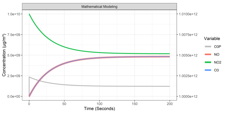
To this end, we used the ode routine of the R package deSolve, which can identify and numerically solve ODE (stiff) systems. Based on the graph shown in Figure 1, as NO₂ is consumed, NO and O₃ are formed. In addition, the equilibrium value is reached quickly, approximately at t=200 seconds. Furthermore, NO₂ and O₃ concentrations approximate when stability is reached, where NO2 consumption is equivalent to the O₃ formed. In other words, to have ozone accumulation in the troposphere, other oxidants must participate in the reactions. The curves shown in Figure 1 are the same as the reference cited above (Figure 12.5, Page 443,⁹).

Figure 1
Numerical solution of the mathematical model presented and defined by equations (2.4), (2.5), (2.6), and (2.7) for the tropospheric ozone cycle. The scale of [NO] is the vertical axis on the right, and the value of [O(^3P)] is presented with a multiplicative factor equal to 10⁶.

Finally, using the initial condition and the parameter values, we obtained the numerical stationary solution shown in Figure 1: (1.2194·10³, 1.0048·10¹², 5.1786·10⁹, 4.8213·10⁹), and the equilibrium solution given by (3.10) is (1.2173·10³, 1.0048·10¹², 5.1699·10⁹, 4.8213·10⁹).

Using Table 2, and with the referred inequality being less than the unity, the eigenvalues are λ_1,2=0, λ₃=-10573.3, and λ₄=-61625.7. According to the theoretical results, this equilibrium solution is stable. Thus, with this computational simulation, we can graphically verify the fulfillment of the theoretical result that was obtained analytically.

4 CONCLUSION

In this work, we present a qualitative study of a mathematical model of ordinary differential equations in time that characterizes the kinetics of the chemical reactions of the ozone cycle in the troposphere. The only equilibrium state of the system is non hyperbolic, and so we used the Center Manifold Theorem to study its local stability. We present complete analytical results that establish that the steady state is stable for any values of the kinetic parameters, which was also corroborated by the numerical solution of the resulting stiff problem. In addition to establishing this unprecedented result of stability, another conclusion is that the simplified model of ozone kinetics with fixed kinetic parameters does not allow the behavior of sustained oscillatory solutions for the referred concentrations of pollutants, requiring other ingredients for this to be feasible. In future works, we intend to address the problem of estimating mathematical model parameters from real data.

ACKNOWLEDGMENTS

JKC thanks PIBIC-CNPq for the Undergraduate Research Scholarship. TSFA thanks UNICAMP and DOW Brasil for the participation in the DOW-“CRIE” (Science, Representativeness, Inclusion, and Experience) Program and for the Undergraduate Research Scholarship of the Charities Aid Foundation America, Inc. (“CAF America”). EMDM and DSR thank the Graduate Program in Technology at UNICAMP and the Coordination for the Improvement of Higher Education Personnel (CAPES) for the Postdoctoral Scholarship of the Graduate Development Program (PDPG), CAPES Strategic Postdoctoral Program (PDPG/CAPES). The authors thank Espaço da Escrita - Pró-Reitoria de Pesquisa - UNICAMP - for the language services provided.

REFERENCES

• ¹ M.I. Abdurrahman, S. Chaki & G. Saini. Stubble burning: effects on health & environment, regulations and management practices. Environmental Advances, 2 (2020), 100011. doi: 10.1016/j.envadv.2020.100011.
  » https://doi.org/10.1016/j.envadv.2020.100011
• ² C. Baird & M. Cann. “Environmental Chemistry”. Bookman, 4 ed. (2011), 650 p.
• ³ P.M. Campos, A.F. Esteves, A.A. Leitão & J.C. Pires. Design of air quality monitoring network of Luanda, Angola: Urban air pollution assessment. Atmospheric Pollution Research, 12(8) (2021), 101128. doi: 10.1016/j.apr.2021.101128.
  » https://doi.org/10.1016/j.apr.2021.101128
• ⁴ J. Carr. “Applications of Centre Manifold Theory”. Applied Mathematical Sciences, 35, Springer New York, NY, 1 ed. (1982).
• ⁵ A. Dessler. “The Chemistry and Physics of Stratospheric Ozone”, volume 74. International Geophysics Series. Academic Press, New York, 2 ed. (2000).
• ⁶ A. Ducrot, Q. Griette, Z. Liu & P. Magal. “Positivity and Invariant Sub-Regions”. Springer International Publishing, Cham (2022), p. 213-223. doi: 10.1007/978-3-030-98136-5_7.
  » https://doi.org/10.1007/978-3-030-98136-5_7
• ⁷ EPA (US Environmental Protection Agency). Guidance on the Development, Evaluation, and Application of Environmental Models (EPA/100/K-09/003) (2009). Council for Regulatory Environmental Modeling. Washington, DC: Office of the Science Advisor.
• ⁸ G. Geidel & W.E. Winner. Environmental Science: the Interdisciplinary STEM field. Journal of Environmental Studies and Sciences, 2(6) (2016), 336-343.
• ⁹ M.Z. Jacobson. “Fundamentals of Atmospheric Modeling”. Cambridge University Press, 2 ed. (2005). doi: 10.1017/CBO9781139165389.
  » https://doi.org/10.1017/CBO9781139165389
• ¹⁰ L.V. Kalachev & R.J. Field. Reduction of a Model Describing Ozone Oscillations in the Troposphere: Example of an Algorithmic Approach to Model Reduction in Atmospheric Chemistry. Journal of Atmospheric Chemistry, 39(1) (2001), 65-93. doi: 10.1023/a:1010649217616.
  » https://doi.org/10.1023/a:1010649217616
• ¹¹ N.A. Manan, A.N. Aizuddin & R. Hod. Effect of Air Pollution and Hospital Admission: A Systematic Review. Annals of Global Health, 84(4) (2018), 670-678.
• ¹² S. Marsili-Libelli. Simplified kinetics of tropospheric ozone. Ecological Modelling, 84(1-3) (1996), 233-244. doi: 10.1016/0304-3800(94)00129-4.
  » https://doi.org/10.1016/0304-3800(94)00129-4
• ¹³ C. Mullen, A. Flores, S. Grineski & T. Collins. Exploring the distributional environmental justice implications of an air quality monitoring network in Los Angeles County. Environmental Research, 206 (2022), 112612. doi: 10.1016/j.envres.2021.112612. URL https://doi.org/10.1016/j.envres.2021.112612
  » https://doi.org/10.1016/j.envres.2021.112612» https://doi.org/10.1016/j.envres.2021.112612
• ¹⁴ K. Na, K.C. Moon & Y. Kim. Source contribution to aromatic VOC concentration and ozone formation potential in the atmosphere of Seoul. Atmospheric Environment, 39 (2005), 5517-5524. doi: 10.1016/j.atmosenv.2005.06.005.
  » https://doi.org/10.1016/j.atmosenv.2005.06.005
• ¹⁵ NRC (National Research Council). Models in Environmental Regulatory Decision Making (2007). Committee on Models in the Regulatory Decision Process, Board on Environmental Studies and Toxicology, Division on Earth and Life Studies. Washington, DC: National Academies Press.
• ¹⁶ L. Perko. “Differential Equations and Dynamical Systems”. Springer-Verlag, New York, 3 ed. (2000).
• ¹⁷ L.K. Peters. Gases and their Precipitation Scavenging in the Marine Atmosphere. In “Air-Sea Exchange of Gases and Particles”. Springer Netherlands (1983), p. 173-240.
• ¹⁸ A. Rathod, S. Sahu, S. Singh & G. Beig. Anomalous behaviour of ozone under COVID-19 and explicit diagnosis of O3-NOx-VOCs mechanism. Heliyon, 7(2) (2021), e06142. doi: 10.1016/j.heliyon.2021.e06142.
  » https://doi.org/10.1016/j.heliyon.2021.e06142
• ¹⁹ J. Roux. “Encyclopedia of Life Support Systems”, volume 2. EOLSS Publishers/UNESCO, Oxford (2009), chapter Mathematical Models in Air Quality Problems.
• ²⁰ A. Salvo & F.M. Geiger. Reduction in local ozone levels in urban São Paulo due to a shift from ethanol to gasoline use. Nature Geoscience, 6(7) (2014), 450-458.
• ²¹ J.H. Seinfeld & S.N. Pandis. “Atmospheric Chemistry and Physics: From Air Pollution to Climate Change”. John Wiley & Sons, Hoboken, New Jersey, 3 ed. (2016).
• ²² S. Sillman. The relation between ozone, NOx and hydrocarbons in urban and polluted rural environments. Atmospheric Environment, 33 (2002), 1821-1845.
• ²³ J. Stoer & R. Bulirsch. “Introduction to Numerical Analysis. Text in Applied Mathematics”. Springer-Verlag, New York, 2 ed. (1991).
• ²⁴ A.C. Targino, R.M. Harrison, P. Krecl, P. Glantz, C.H. de Lima & D. Beddows. Surface ozone climatology of South Eastern Brazil and the impact of biomass burning events. Journal of Environmental Management, 252 (2019), 109645. doi: https://doi.org/10.1016/j.jenvman.2019.109645. URL https://www.sciencedirect.com/science/article/pii/S0301479719313635
  » https://doi.org/10.1016/j.jenvman.2019.109645» https://www.sciencedirect.com/science/article/pii/S0301479719313635
• ²⁵ H. Tian, R. Xu, J.G. Canadell, R.L. Thompson, W. Winiwarter, P. Suntharalingam, E.A. Davidson, P. Ciais, R.B. Jackson, G. Janssens-Maenhout, M.J. Prather, P. Regnier, N. Pan, S. Pan, G.P. Peters, H. Shi, F.N. Tubiello, S. Zaehle, F. Zhou, A. Arneth, G. Battaglia, S. Berthet, L. Bopp, A.F. Bouwman, E.T. Buitenhuis, J. Chang, M.P. Chipperfield, S.R.S. Dangal, E. Dlugokencky, J.W. Elkins, B.D. Eyre, B. Fu, B. Hall, A. Ito, F. Joos, P.B. Krummel, A. Landolfi, G.G. Laruelle, R. Lauerwald, W. Li, S. Lienert, T. Maavara, M. MacLeod, D.B. Millet, S. Olin, P.K. Patra, R.G. Prinn, P.A. Raymond, D.J. Ruiz, G.R. van der Werf, N. Vuichard, J. Wang, R.F. Weiss, K.C. Wells, C. Wilson, J. Yang & Y. Yao. A comprehensive quantification of global nitrous oxide sources and sinks. Nature, 586(7828) (2020), 248-256. doi: 10.1038/s41586-020-2780-0. URL https://doi.org/10.1038/s41586-020-2780-0
  » https://doi.org/10.1038/s41586-020-2780-0» https://doi.org/10.1038/s41586-020-2780-0
• ²⁶ M. Travaglio, Y. Yu, R. Popovic, L. Selley, N.S. Leal & L.M. Martins. Links between air pollution and COVID-19 in England. Environmental Pollution, 268 (2021), 115859. doi: https://doi.org/10.1016/j.envpol.2020.115859. URL http://www.sciencedirect.com/science/article/pii/S0269749120365489
  » https://doi.org/10.1016/j.envpol.2020.115859» http://www.sciencedirect.com/science/article/pii/S0269749120365489
• ²⁷ D. Vallero. “Fundamentals of Air Pollution”. Academic Press, Oxford, 5 ed. (2014).
• ²⁸ J. Wainwright & M. Mulligan. “Environmental Modelling: Finding Simplicity in Complexity”. John Wiley & Sons, Oxford, 2 ed. (2012).
• ²⁹ World Health Organization. URL https://www.who.int/air-pollution
  » https://www.who.int/air-pollution
• ³⁰ World Health Organization. “WHO global air quality guidelines: particulate matter (PM2.5 and PM10), ozone, nitrogen dioxide, sulfur dioxide and carbon monoxide”. World Health Organization (2021), xxi, 273 p.

• 1
  According to the definition of the US National Research Council, and not only in the mathematical scope, a model is “a simplification of reality that is constructed to gain insights into select attributes of a particular physical, biological, economic, or social system”¹⁵.

Publication Dates

• Publication in this collection
  10 Feb 2025
• Date of issue
  2025

History

• Received
  19 Dec 2023
• Accepted
  26 Nov 2024