Machine learning application in geotechnics: predicting sand behavior with direct shear tests

Abstract

In geotechnical engineering, soil strength parameters are fundamental to design. Field and laboratory tests are essential, yet they often involve practical and financial constraints. Traditional approaches based on empirical or theoretical relationships may not adequately capture the complexity of soil behavior. This study investigates the use of artificial intelligence as an alternative approach to address these limitations. A predictive model was developed to represent the stress–strain response obtained from direct shear tests on sandy materials. Data compiled and digitized from multiple published sources were used to build an experimental dataset for training three machine learning (ML) algorithms: Support Vector Regression (SVR), Random Forest (RF), and Feedforward Neural Network (FNN). The models were evaluated using performance metrics and validation test curves. Among them, RF produced the most consistent performance. SVR and FNN also showed satisfactory results, although to a lesser extent. These findings indicate that ML techniques, particularly RF, can provide useful support for geotechnical engineers and researchers in predicting the behavior of sands, even when working with a relatively limited dataset.

Keywords:
Artificial Intelligence; Direct shear; Predictive model; Machine learning; Geotechnical laboratory test

1. Introduction

Understanding the shear strength of soil is fundamental for geotechnical engineering, as it directly affects the stability and safety of civil structures. Lambe & Whitman (1969) emphasize that the shear strength of dry granular soils is influenced by several factors, which may be grouped into two categories. The first includes factors that affect a specific soil, such as void ratio, confining stress, and loading rate. The second covers factors that distinguish the strength of one soil from another, even when stresses and void ratio are comparable, including particle size, particle shape, and grain size distribution.

The determination of shear strength parameters is essential for geotechnical analyses and design. Traditionally, these parameters are obtained through field and laboratory tests supported by empirical or theoretical relationships. However, such approaches may not fully represent the complexity of soil behavior.

Artificial intelligence (AI) has emerged as a promising tool in this context. Recent computational techniques, including AI, have been applied to various problems in geosciences and geotechnical engineering (Kanungo et al., 2014). Building on this trend, the present study develops and evaluates predictive models based on Machine Learning (ML) techniques, including Random Forest (RF), Support Vector Regression (SVR), and Feedforward Neural Networks (FNN), to estimate stress–strain curves obtained from direct shear tests on sand.

2. Literature review

2.1 Shear strength of soils

The study of soil strength is directly related to the stress state that leads to failure. According to Lambe & Whitman (1969), failure criteria describe the conditions under which materials fail under compression, tension, shear stresses, or strain energy. The Mohr–Coulomb criterion, widely used in geotechnical engineering, combines the formulations of Mohr and Coulomb; failure is reached when the Mohr stress circle touches the failure envelope defined by Coulomb’s equation. In sands, due to their high permeability, pore pressure dissipates almost instantaneously, and no excess pore pressure is generated ($\Delta u=0$).

Lambe & Whitman (1969) note that drained triaxial tests are the most appropriate method for analyzing the behavior of monotonic sands. In isotropically consolidated and drained (CID) triaxial compression tests, sands may display either contractive behavior, characterized by volumetric reduction, or dilative behavior, associated with volumetric increase. This response depends on the initial void ratio ($e_0$), relative density (RD), and the effective confining stress (${\sigma }_c^{\text{'}}=0$) at the onset of shearing.

Under contractive behavior, increasing axial strain produces a gradual rise in deviator stress until reaching a maximum value. Tests performed under different confining stresses show a proportional relationship between the deviator stress and the confining stress, resulting in a failure envelope that passes through the origin. Under dilative behavior, the deviator stress reaches a peak and then decreases until stabilizing at the residual strength. Dilation typically occurs after a brief initial contraction and is more pronounced under lower confining stresses (Lambe & Whitman, 1969).

2.2 Effect of void ratio and confining stress on sand behavior

Lee & Seed (1967) conducted isotropically consolidated and drained triaxial compression tests on Sacramento River sand. Samples prepared in loose and dense conditions were subjected to different confining stress levels (${\sigma }_c$). For dense conditions, increasing the confining stress produced three main effects: a reduction in peak stresses, an increase in axial strain at failure, and a decrease in dilatancy. Under sufficiently high stresses, even dense specimens may undergo volumetric compression. For loose conditions, similar trends were observed, but with lower dilatancy at low confining stresses and greater compression at higher stresses, demonstrating the influence of initial density on the mechanical behavior of sand (Lee & Seed, 1967).

2.3 Laboratory tests

Laboratory tests are essential for investigating the physical and mechanical properties of soils (Corte et al., 2017). Common procedures include the direct shear test, triaxial compression test, ring shear test, cubic triaxial test, hollow cylinder test, and direct simple shear (DSS) test. The present study focuses on the direct shear test.

According to Corte et al. (2017), as published in Soils and Rocks, the direct shear test is one of the most traditional methods for evaluating shear strength based on the Mohr–Coulomb criterion. The test is known for being rapid, cost-effective, and relatively simple for determining geotechnical parameters. In this procedure, normal stress is applied to a predefined plane, and the shear stress required to induce failure is measured. The split box mechanism enables controlled horizontal displacement, and the resulting data are used to generate shear strength curves. One limitation of the test is the inability to control drainage conditions, meaning that results are interpreted in terms of total stresses.

2.4 Machine learning

2.4.1 Basic concepts of machine learning

Artificial intelligence encompasses a wide range of approaches, often associated with simulating human performance or developing systems that behave rationally. Among its subfields, one of the most influential is machine learning, which focuses on creating algorithms that learn from data and improve their performance without explicit reprogramming (Russell & Norvig, 2020). The effectiveness of ML models depends strongly on both the quality and the quantity of data available (Mohri et al., 2018).

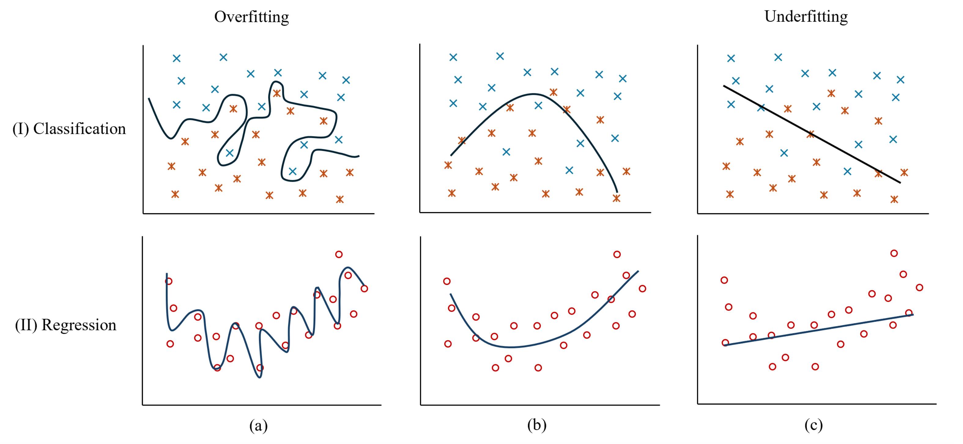
Machine learning methods are commonly divided into supervised and unsupervised learning. In supervised learning, algorithms rely on labeled examples and are widely used in classification and regression tasks. Classification, as illustrated in Figure 1a, involves labeling data into predefined categories, such as sorting emails into “spam” or “not spam”. Regression, shown in Figure 1b, aims to predict continuous values, such as estimating material strength or house prices (Mohri et al., 2018).

Figure 1
Classification and regression models with different fits: (a) overfitting; (b) adequate fit; (c) underfitting. Adapted from MathWorks (2024).

During model development, a dataset containing inputs and corresponding outputs is provided so the algorithm can learn to generate accurate predictions. After training, the model is validated to adjust its parameters and then tested on new data to assess its generalization capability. A model that performs well on unseen data is considered well-fitted. A common challenge in model development involves addressing underfitting and overfitting (Baranauskas & Monard, 2000). Underfitting, shown in Figure 1c, occurs when the model fails to capture essential patterns in the data. Overfitting, illustrated in Figure 1a, arises when the model captures noise or specific irregularities, reducing its ability to generalize. Ideally, the model should achieve a balance between simplicity and complexity, as represented in Figure 1b.

2.4.2 Application of machine learning in geotechnics

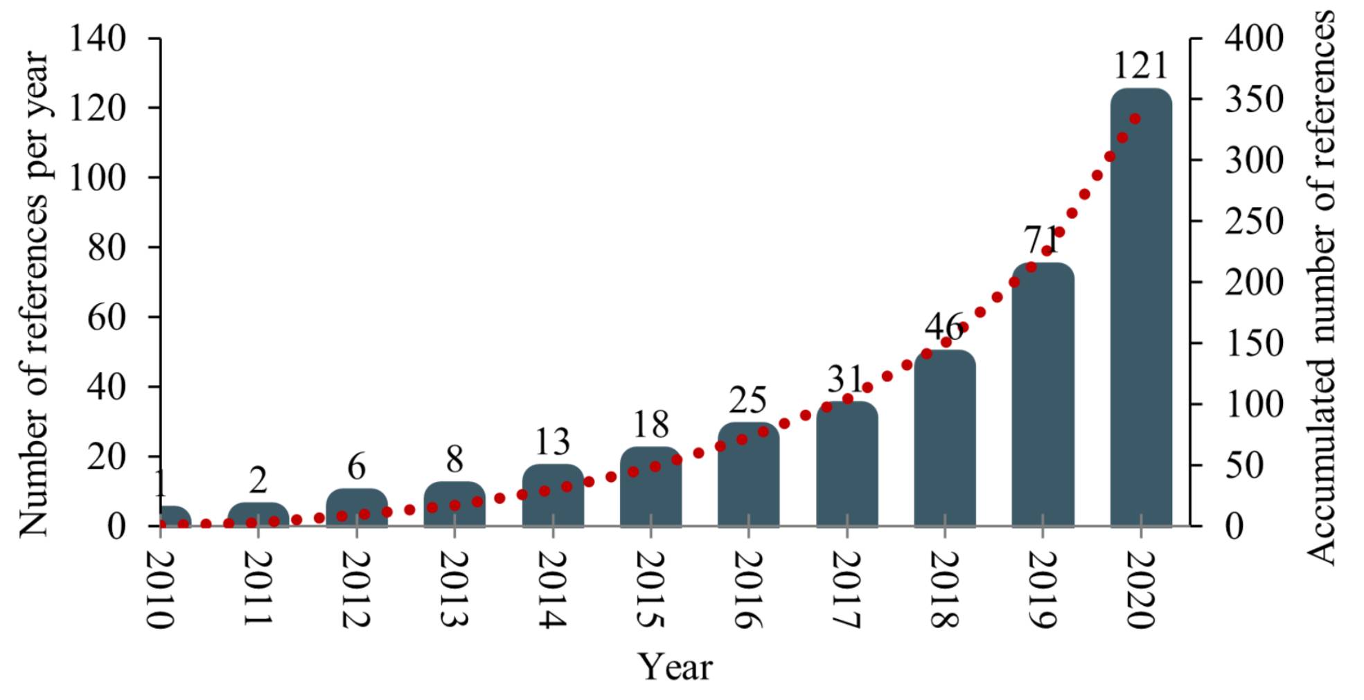
Zhang et al. (2022) analyzed the growing use of machine learning in predicting soil properties, as shown in Figure 2, highlighting a significant rise in applications in engineering and geology since 2018. Examples include the use of Support Vector Regression (SVR) to predict landslide displacement (Wang et al., 2023), k-Nearest Neighbors (k-NN) to estimate soil moisture from laboratory and environmental parameters (Yamaç et al., 2020), and Feedforward Neural Networks (FNN) to forecast surface settlement induced by shield tunneling (Chen et al., 2019). Collectively, these studies illustrate the increasing adoption of ML techniques in geotechnical engineering.

Figure 2
Number of publications related to the development and application of machine learning algorithms for soil property prediction. Adapted from Zhang et al. (2022).

In the context of deep learning, Zhang et al. (2021) reported a rapid increase in publications over the past decade, with applications across several geotechnical domains. Examples include Artificial Neural Networks (ANN) used to predict pile settlement (Nejad et al., 2009) and soil liquefaction (Baziar & Jafarian, 2007), as well as Convolutional Neural Networks (CNN) applied to estimate P-wave and S-wave velocities in rocks (Karimpouli & Tahmasebi, 2019).

In Brazil, the literature also documents notable progress in applying machine learning to geotechnical problems. Examples include Random Forest models developed to estimate the pile spring coefficient (Oliveira et al., 2020), ANNs applied to predict foundation settlements (Araújo, 2015), and the development of a multilayer ANN model to estimate hydraulic conductivity (Silva, 2020). Carvalho et al. (2022) reviewed 18 studies published between 2008 and 2018 on the use of artificial intelligence to estimate soil shear strength. These works demonstrate the flexibility and efficiency of ML techniques, even when dealing with relatively limited datasets, which is a common condition in geotechnical engineering.

2.4.3 Random forest (RF)

Decision trees are machine learning techniques that partition the feature space into simplified regions, using the mean or mode of the training observations to generate predictions (James et al., 2023). Random Forests consist of multiple decision trees operating collectively. Each tree is built using randomly selected feature subsets, and in classification tasks, the forest predicts the most frequent class across all tree votes (Breiman, 2001). According to Zhang et al. (2022), a Random Forest aggregates the predictions of multiple independently constructed trees, forming a “committee” whose combined decision generally improves predictive performance. In regression problems, the final output corresponds to the average of all tree predictions.

Training an RF begins with the original dataset and involves generating multiple bootstrap samples, each used to construct an individual tree. The results are then aggregated to form the final prediction. RFs have gained prominence due to their efficiency, scalability, and ease of implementation. Tree construction relies on bagging (bootstrap aggregating), where several training sets are produced through sampling with replacement. Typically, each bootstrap sample contains about two-thirds of the original data, leaving the remaining one-third as “out-of-bag” observations for error estimation and performance assessment (Raschka & Mirjalili, 2017).

2.4.4 Support vector regression (SVR)

Support Vector Machines (SVM) are grounded in statistical learning theory, which provides principles for constructing classifiers with strong generalization capability. Generalization refers to a model’s ability to correctly classify or predict outcomes for new data drawn from the same domain as the training set (Lorena & Carvalho, 2007). Figure 3 presents an overview of the SVM structure.

Figure 3
The soft margin loss setting for a linear SVM. Adapted from Schölkopf & Smola (2002 apud Smola & Schölkopf, 2004).

Support Vector Regression, an SVM variant designed for regression tasks, seeks to minimize prediction error while maximizing the margin, incorporating flexibility through slack variables ($\xi$) that allow deviations within a specified tolerance $\epsilon$. The support vectors, which are the data points closest to the hyperplane, play a central role in defining this margin. During training, the objective is to identify a hyperplane that fits the data with the largest possible margin while permitting controlled error. The SVR formulation discussed in Zhang et al. (2022) is presented in Equation 1, where m denotes the number of observations, $\xi$ represents the slack parameters, and C is the regularization constant. A commonly used kernel function is given in Equation 2, where ${\gamma }_{kernel}$ is the kernel coefficient.

$$\begin{array}{l}mi{n}_{\xi ,w,b}\frac{1}{2}{\left|\left|W\right|\right|}^2+C{{\displaystyle \sum }}_{i=1}^m{\xi }_i\\ s.a.y_i\left(W^T\varphi \left(X\right)+b\right)\ge 1-{\xi }_i,i=\mathrm{1,2,}\dots ,m,{\xi }_i\ge 0\end{array}$$ (1)

$\varphi \left(x_i,x_j\right)=expexp\left(-{\gamma }_{kernel}{\left|\left|x_i-x_j\right|\right|}^2\right)$ (2)

2.4.5 Feedforward neural network (FNN)

A simplified neuron model in an Artificial Neural Network (ANN) draws inspiration from biological neurons, which receive stimuli, process signals through synaptic weights, and generate outputs according to their activation levels (Fielding, 1999). Interactions among network layers are a defining feature of ANNs and distinguish them from linear or rule-based decision models (Russell & Norvig, 2020).

Several ANN architectures exist, including Feedforward Neural Networks, Convolutional Neural Networks, and Recurrent Neural Networks (Russell & Norvig, 2020; James et al., 2023). Among these, FNNs are widely used in machine learning due to their simplicity and effectiveness. They typically consist of input, hidden, and output layers (Zhang et al., 2022). The present study focuses on FNNs. Figure 4 shows an example of an FNN configuration with one hidden layer.

Figure 4
Example of FNN network with one hidden layer. Adapted from James et al. (2023).

Mathematically, an FNN can be represented by Equations 3 and 4. The network processes input vectors $X_1$, $X_2$, … , $X_p$ through a function $f\left(X\right)$ to predict the output $Y$. Hidden layer activations, denoted by $A_k$, are computed from the inputs using nonlinear activation functions $g\left(z\right)$, such as the sigmoid or ReLU function, resulting in $h_k\left(X\right)$. These activations contribute to generating the network output. During training, the parameters associated with the model (weights $W$ and biases $\beta$) are adjusted to minimize prediction error. Nonlinear activation functions are essential for enabling the model to capture complex relationships in the data (James et al., 2023).

$\begin{array}{c}f\left(X\right)={\beta }_0+{{\displaystyle \sum }}_{k=1}^K\\ {\beta }_k{h}_k\left(X\right)={\beta }_0+{{\displaystyle \sum }}_{k=1}^K\\ {\beta }_{k}g\left(W_{k0}+{{\displaystyle \sum }}_{j=1}^p{W}_{kj}{X}_j\right)\end{array}$ (3)

$A_k=h_k\left(X\right)=g\left(W_{k0}+{{\displaystyle \sum }}_{j=1}^p{W}_{kj}{X}_j\right)$ (4)

2.5 Model performance evaluation

In machine learning, no single algorithm performs best for all problems, making it essential to understand the strengths and limitations of each method (Baranauskas & Monard, 2000). The goal is to select the hypothesis that best fits the data while minimizing errors on future observations (Russell & Norvig, 2020). A common strategy is to evaluate a variety of algorithms and use separate datasets for training, validation, and final testing to ensure an unbiased assessment of model performance (Baranauskas & Monard, 2000; Russell & Norvig, 2020).

Two widely used metrics in regression tasks are the Mean Absolute Error (MAE) and the Root Mean Square Error (RMSE). MAE, presented in Equation 5, computes the average absolute difference between predicted and actual values. RMSE, given in Equation 6, calculates the square root of the mean squared error and places greater emphasis on larger deviations. Unlike RMSE, which is sensitive to outliers, MAE behaves similarly to the Manhattan norm, reflecting distance along orthogonal axes. Both metrics measure the deviation between predictions and observed values (Baranauskas & Monard, 2000; Géron, 2019).

$MAE=\frac{1}{n}{{\displaystyle \sum }}_{i=1}^n\left|y_i-h\left(x_i\right)\right|$ (5)

$RMSE=\sqrt{\frac{1}{n}{{\displaystyle \sum }}_{i=1}^n{\left(y_i-h\left(x_i\right)\right)}^2}$ (6)

The coefficient of determination ($R^2$), shown in Equation 7, is a statistical metric that quantifies the proportion of variance in the observed data explained by the model. It ranges from 0 to 1 and is independent of the scale of the dependent variable (James et al., 2023). This metric is also frequently used to assess predictive performance in machine learning models.

$R^2=1-\frac{{{\displaystyle \sum }}_{i=1}^n{\left(y_i-\widehat{\{h{(x\}}_i)}\right)}^2}{{{\displaystyle \sum }}_{i=1}^n{\left(y_i-\underset{\_}{y}\right)}^2}$ (7)

3. Materials and methods

3.1 Materials

A comprehensive online search was conducted using keywords related to direct shear tests. The search included scientific articles, conference papers, undergraduate theses, master’s dissertations, and doctoral theses that reported experimental results in the form of stress–strain graphs. Publications that did not provide such data were excluded. In the subsequent screening stage, only documents aligned with the scope of this study were retained. Because the focus was on sandy materials under dry or fully saturated conditions, studies involving other materials—such as tailings, glass beads, clays, or clay mixtures—were excluded due to their distinct mechanical behavior compared with sand.

From this process, seven studies were selected, comprising 205 individual tests and yielding 7,185 stress–strain data pairs. Three of these tests were reserved for model validation. To ensure that validation data originated from different sources, the dataset was divided into three segments, and one test from each segment was randomly selected. After interpolation and the application of a horizontal displacement threshold, and excluding validation data, a total of 3,434 data points were retained. Table 1 summarizes the selected studies, including authors, publication year, title, location, and number of contributing tests.

Table 1
Summary of studies used in direct shear models.

Author	Study Title	Sand Location	Number of Tests
Coutinho (2021)	Direct Shear Tests on Ipanema Beach Sand	Ipanema	71
Marques & Oliveira (2009)	Hokksund Sand Tests for Calibration Chamber Revitalization Project	Hokksund	20
Monteiro et al. (2023)	Geotechnical Characterization of the Sand from Porto do Açu	Porto do Açu	16
Nunes (2014)	Geotechnical characterization tests on sand from Itaipuaçu beach	Itaipuaçu	29
Pinheiro (2018)	Geotechnical characterization in the laboratory of sand from Cavaleiros beach – Macaé/RJ	Cavaleiros	24
Simões (2015)	Geotechnical characterization of Ipanema beach sand	Ipanema	30
Teles (2013)	Study on the strength and deformability parameters of Hokksund sand	Hokksund	15

3.2 Methods

The methodology consisted of four main stages: (I) data collection, (II) data preprocessing, (III) model architecture definition and training, and (IV) performance analysis and validation.

3.2.1 Data collection

Following the selection of relevant studies described in Section 3.1, data were gathered through a systematic procedure involving three steps: graphical data acquisition, data digitization, and supplementary information extraction.

• Graphical Data Acquisition: Stress–strain graphs from the selected studies were isolated and exported as individual images for processing;

• Data Digitization: The software PlotDigitizer (2023) was used to convert the extracted graphs into numerical stress–displacement pairs. The digitized points were subsequently reviewed in Excel, where they were overlaid on the original figures to verify accuracy;

• Supplementary Information Analysis: Each study was examined to collect additional parameters, such as initial void ratio and applied vertical stress, to provide experimental context for each test.

These procedures were conducted individually for each study and combined into a consolidated dataset.

3.2.2 Data preprocessing

Data preprocessing was performed to ensure data quality, consistency, and suitability for machine learning. This phase involved cleaning, organizing, and transforming the dataset to accurately represent the experimental conditions.

An initial exploratory assessment was conducted through visual inspection of individual and combined stress–strain curves. This allowed identification of inconsistencies stemming from digitization, such as typographical errors or incorrect axis assignments. Detected issues were corrected to maintain reliability.

For standardization, uniform acquisition intervals were generated using interpolation, producing regularly spaced data points, and enabling consistent comparisons across studies. These interpolated curves were validated against the original graphs to ensure that the essential characteristics were preserved. A consistent final horizontal displacement value was also defined for all tests.

Finally, all input variables were normalized so that they fell within a common numerical range, reducing scale-related bias and ensuring balanced contributions of each parameter during model training.

3.2.3 Model architectures and training

Selecting appropriate hyperparameters is essential for improving predictive performance and model generalization. This study employed Grid Search to identify optimal hyperparameter combinations for each regression model. Using the GridSearchCV tool from Python’s scikit-learn library, a grid of candidate values was defined and evaluated through three-fold cross-validation.

Model performance was assessed using metrics such as MAE, RMSE, and $R^2$. Once optimal hyperparameters were identified, the models were trained on the preprocessed dataset, adjusting their internal parameters iteratively to minimize prediction error

3.2.4 Performance analysis and validation

Model validation was carried out using the regression metrics MAE, RMSE, and $R^2$. Evaluating the models on unseen data allowed assessment of generalization and identification of potential error patterns. Because a single metric may not fully represent model suitability, the evaluation considered the problem context and relative performance across metrics.

The validation set was also used to predict shear stress–strain curves, providing practical insight into the models’ ability to reproduce direct shear test behavior. Comparative analysis of the results enabled the identification of the best-performing model.

Python was selected due to its robust ecosystem of machine learning libraries, including pandas for data manipulation, NumPy for numerical computation, scikit-learn for model implementation, TensorFlow and Keras for neural network training, and Matplotlib and Seaborn for data visualization.

4. Results analysis

4.1 Models

The database was organized into categories to support the interpretation of soil properties and behavior. The established categories include material location, soil physical properties, specimen preparation conditions, and test results, as outlined below:

• Material Location: Identifies the source of the soil;

• Soil Physical Properties: Incorporates maximum void ratio ($e_{max}$), minimum void ratio ($e_{min}$), and specific gravity ($G_s$);

• Specimen Preparation Conditions: Includes average initial void ratio ($e_0$) and relative density ($RD$);

• Test Results: Covers consolidation stress (${\sigma }_v$), corrected specimen area, shear rate, horizontal displacement (${\delta }_h$), shear stress ($\tau$), and shear ratio ($\tau /{\sigma }_v$).

Due to variations in parameter availability among studies, parameters with missing values were excluded to maintain consistency. Some variables used only for sample identification were also not included in the predictive analysis. The model inputs and their statistical summaries are presented in Table 2.

Table 2
Minimum and maximum input and output values for parameters used in models.

	Input (X)					Target (y)
	$G_s$	$e_0$	$RD\left(\%\right)$	${\sigma }_v\left(kPa\right)$	${\delta }_h\left(mm\right)$	$\tau /{\sigma }_v$
min	2.643	0.428	8	12.50	0	-
max	2.763	0.726	99	1600.00	5	-

As part of preprocessing, digitized curves were overlaid on their corresponding original graphs to verify accuracy. Individual and combined plots were also generated to detect anomalies.

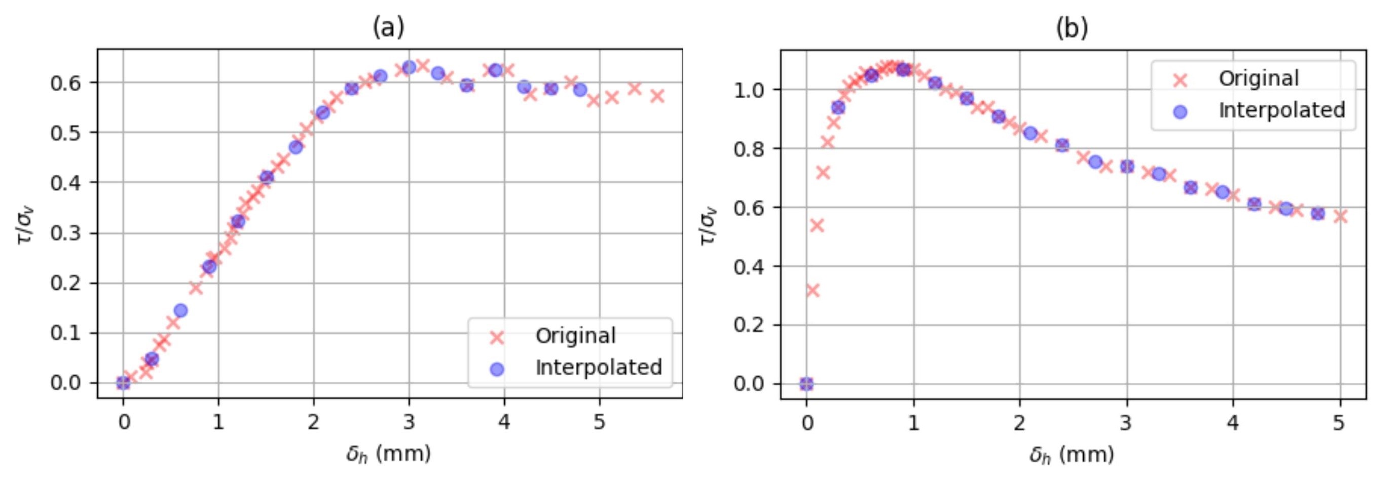
To address inconsistencies in horizontal displacement (${\delta }_h$) values, a standard displacement limit of 5 mm was adopted for all tests. Irregular acquisition intervals were standardized through interpolation, using 0.3 mm increments for direct shear tests. After interpolation, both individual plots (Figures 55b) and collective plots (Figures 66b) were reviewed to confirm accuracy. Figure 6a illustrates all curves before preprocessing, while Figure 6b shows the same curves after preprocessing.

Figure 5
Individual plots showing original and interpolated data points for interpolation verification in two examples: (a) Test 1; (b) Test 2.

Figure 6
Plots of all tests superimposed: (a) before data preprocessing; (b) after data preprocessing.

The dataset was divided into training, testing, and validation groups. For the validation set, random samples were selected to ensure that no more than one test originated from the same study. The remaining data were split into 80% for training and 20% for testing. During training, the horizontal displacement interval on the x-axis remained fixed, and the models were trained to predict normalized shear stress ($\tau /{\sigma }_v$).

4.2 Performance analysis

The analysis consisted of quantitative and qualitative evaluations. The quantitative evaluation used the training and testing datasets to assess model performance through statistical metrics, whereas the qualitative evaluation focused on complete validation tests, examining whether the predicted curves reproduced key sand responses such as contraction and dilation. This combined approach provided a comprehensive assessment of each model’s capability to represent realistic soil behavior.

4.2.1 Quantitative analysis of training and testing data

After training the models with their respective optimal hyperparameters, the Mean Absolute Error (MAE), Root Mean Square Error (RMSE), and coefficient of determination ($R^2$) were computed for both training and testing sets. Results are shown in Table 3.

Table 3
Performance metrics in train and test data.

	Train			Test
	MAE	RMSE	R 2	MAE	RMSE	R 2
RF	0.01	0.02	0.99	0.03	0.05	0.96
SVR	0.05	0.10	0.86	0.06	0.10	0.85
FNN	0.09	0.13	0.75	0.09	0.13	0.74

The RF model exhibited the strongest performance, with very low MAE and RMSE values in training (0.01 and 0.02, respectively) and an $R^2$ of 0.99, indicating near-perfect agreement with the data. In testing, RF showed only a modest increase in error (MAE 0.03; RMSE 0.05) and maintained a high $R^2$ of 0.96, demonstrating strong generalization.

SVR and FNN performed worse than RF. FNN showed higher error values during training (MAE 0.09; RMSE 0.13) and a lower $R^2$ of 0.74, consistent across testing. SVR achieved intermediate performance.

Overall, RF consistently delivered the best results, suggesting it is the most suitable model for the analyzed dataset. SVR and FNN produced acceptable outcomes but with noticeably reduced accuracy.

4.2.2 Qualitative analysis of validation data

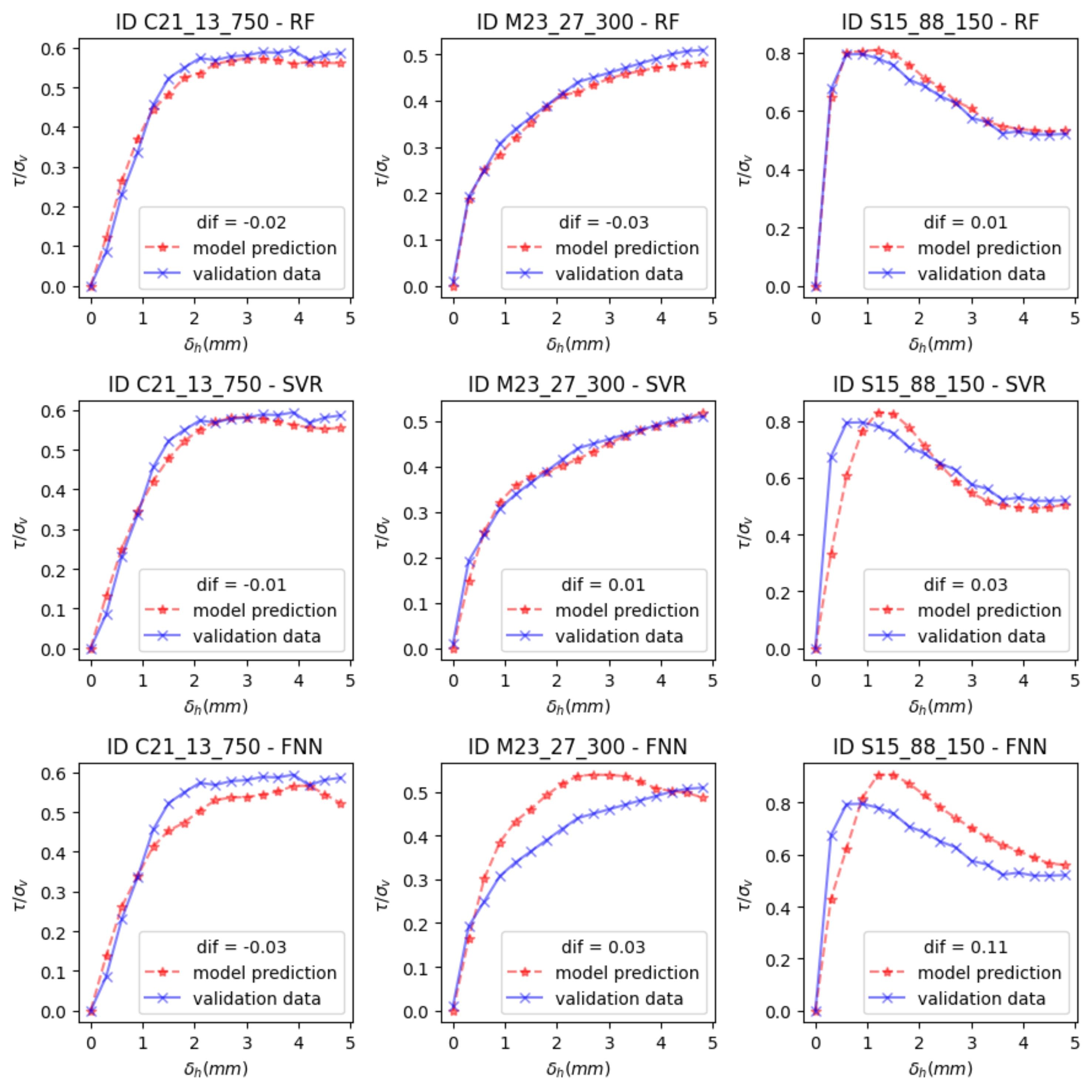
The predicted shear stress–strain curves for the validation tests are shown in Figure 7, with model predictions in red and validation data in blue. Three full validation tests were randomly selected. To complement visual assessment, an additional measure was used to evaluate model conservatism for geotechnical applications. This indicator compares the maximum predicted shear stress to the maximum value from the corresponding validation test, as defined in Equation 8. Positive values indicate overestimation, a desirable condition in safety-oriented analyses.

Figure 7
Prediction curves in the validation data of the three models in the direct shear tests.

$dif=max\left(y_{predicted}\right)-max\left(y_{real}\right)$ (8)

The RF model showed strong agreement with validation curves, effectively reproducing both contractive and dilative responses. Deviations ranged from 0.01 to −0.03, indicating slight underestimation of peak shear stress but good overall alignment across the displacement range.

For the SVR model, predictions were highly accurate for some tests (e.g., ID M23_27_300) but showed minor discrepancies in others (e.g., ID S15_88_150), including a slight post-peak rise not observed in the validation data. Differences ranged from −0.01 to 0.03.

The FNN model showed less consistency compared with RF and SVR. Certain validation tests (e.g., ID M23_27_300) exhibited noticeable deviations, with differences ranging from −0.03 to 0.11, including occasional overestimation of peak shear stress.

Overall, all three models demonstrated potential for predicting shear stress–displacement curves in direct shear tests. RF and SVR showed the most reliable combination of accuracy and practical safety, while FNN may require refinement to achieve consistent results.

5. Conclusion

This study investigated machine learning models for predicting stress–strain curves in geotechnical direct shear tests. Using a dataset of 205 direct shear tests, the models were optimized through grid search and evaluated with data divided into training, testing, and validation sets. The RF model consistently outperformed the other approaches, demonstrating high accuracy and reliable generalization, as indicated by stable $R^2$ values close to unity. Its performance during validation also showed conservative peak stress estimates that closely matched measured values, reinforcing its suitability for geotechnical applications. In contrast, the SVR and FNN models exhibited greater variability in accuracy and generalization, indicating limitations in fully capturing the underlying patterns relative to RF.

Despite the relatively limited dataset, the findings were encouraging and support the feasibility of applying advanced machine learning techniques as complementary tools in geotechnical engineering. The difference metric introduced in this study to evaluate the conservatism of model predictions proved useful for assessing reliability, an essential factor in geotechnical contexts where safety considerations are critical. Because RF produced low difference values and stable behavior, it offers a promising balance of predictive accuracy and conservatism; however, incorporating explicit safety factors in future developments may enhance its practical applicability.

This study demonstrates the potential of machine learning to strengthen traditional geotechnical analyses by improving prediction accuracy and supporting safer design decisions. The RF model showed strong capability in reproducing stress–strain responses in sandy soils, suggesting that machine learning can complement conventional engineering methods by providing reliable insight into soil behavior.

This study also included the development of the GSandy software, which enables users to interact with the trained models to simulate stress–strain curves. The tool provides access to references and the underlying dataset, supporting broader applications and promoting the adoption of machine learning in geotechnical engineering.

List of symbols and abbreviations

$e_0$ Initial void index

$e_{máx}$ Maximum void index

$e_{mín}$ Minimum void index

$f$ Friction coefficient

$f\left(X\right)$ Nonlinear function constructed by the neural network

$g\left(z\right)$ Activation function

$h\left(X\right)$ Hypothesis function

k-NN k-Nearest Neighbors

$u$ Pore pressure

$x_i$ Attributes (or features)

$y_i$ Prediction (or target)

AI Artificial Intelligence

ANN Artificial Neural Network

$C$ Regularization parameter

CAPES Coordination for the Improvement of Higher Education Personnel

CID Consolidated Isotropic Drained

CNN Convolutional Neural Network

DSS Direct Simple Shear

FNN Feedforward Neural Network

$Gs$ Specific gravity of solids

MAE Mean Absolute Error

ML Machine Learning

$R^2$ Coefficient of determination

$RD$ Relative density

RF Random Forest

RMSE Root Mean Squared Error

RNN Recurrent Neural Network

SVM Support Vector Machine

SVR Support Vector Regression

$V$ Volume

$W$ Weight vector

$X_p$ Input vector of p variables

$\beta$ Bias

${\gamma }_{kernel}$ Kernel coefficient

${\delta }_h$ Horizontal displacement

${\delta }_v$ Vertical displacement of the top cap

$\xi$ Slack parameter

$\sigma$ Normal stress

$\sigma {\text{'}}_c$ Confining stress

${\sigma }_v$ Vertical stress

${\sigma }_{v0}$ Initial total vertical stress

$\tau$ Shear stress

$\varphi$ mapping function

Acknowledgements

The authors acknowledge the support from the Brazilian Coordination for the Improvement of Higher Education Personnel (CAPES) – Finance Code 001 (Grant N. E-26/200.140/2023).

• Discussion open until August 31, 2026.
• Data availability
  The datasets generated analyzed during the current study are available from the corresponding author upon request.
• Declaration of use of generative artificial intelligence
  This work was prepared without the assistance of any generative artificial intelligence (GenAI) tools or services. All aspects of the manuscript were developed solely by the authors, who take full responsibility for the content of this publication.

References

• Araújo, C.B.C. (2015). Application of perceptron-type artificial neural networks in settlement estimation in piles [Master’s dissertation]. Federal University of Ceará, Fortaleza (in Portuguese).
• Baranauskas, J. A., & Monard, M. C. (2000). Reviewing some machine learning concepts and methods. São Carlos: ICMC-USP (in Portuguese).
• Baziar, M.H., & Jafarian, Y. (2007). Assessment of liquefaction triggering using strain energy concept and ANN model. Soil Dynamics and Earthquake Engineering, 27(12), 1056-1072. https://doi.org/10.1016/j.soildyn.2007.03.007
  » https://doi.org/10.1016/j.soildyn.2007.03.007
• Breiman, L. (2001). Random forests. Machine Learning, 45(1), 5-32. https://doi.org/10.1023/A:1010933404324
  » https://doi.org/10.1023/A:1010933404324
• Carvalho, M.G., Silva, T.C., Rodrigues, A.C., & Almeida, V. (2022). Applications of artificial intelligence in determining soil shear strength parameters: a systematic literature review. Research, Society and Development, 11(1), e27711124506. https://doi.org/10.33448/rsd-v11i1.24506
  » https://doi.org/10.33448/rsd-v11i1.24506
• Chen, R.P., Zhang, P., Kang, X., Zhong, Z.Q., Liu, Y., & Wu, H.N. (2019). Prediction of maximum surface settlement caused by EPB shield tunneling with ANN methods. Soil and Foundation, 59(2), 284-295. https://doi.org/10.1016/j.sandf.2018.11.005
  » https://doi.org/10.1016/j.sandf.2018.11.005
• Corte, M.B., Festugato, L., & Consoli, N.C. (2017). Development of a cyclic simple shear apparatus. Soils and Rocks, 40(3), 279-289.
• Coutinho, J.V.M. (2021). Direct shear tests on Ipanema Beach sand [Master’s dissertation]. Pontifical Catholic University of Rio de Janeiro, Rio de Janeiro (in Portuguese).
• Fielding, A.H. (1999). Machine learning methods for ecological applications. Boston: Springer. https://doi.org/10.1007/978-1-4615-5289-5
  » https://doi.org/10.1007/978-1-4615-5289-5
• Géron, A. (2019). Hands-on machine learning with Scikit-Learn, Keras, and TensorFlow (2nd ed.). Sebastopol, CA: O’Reilly Media.
• James, G., Witten, D., Hastie, T., Tibshirani, R., & Taylor, J. (2023). An introduction to statistical learning with applications in Python Cham: Springer. https://doi.org/10.1007/978-3-031-38747-0
  » https://doi.org/10.1007/978-3-031-38747-0
• Kanungo, D.P., Sharma, S., & Pain, A. (2014). ANN and CART for indirect estimation of unsaturated soil shear strength parameters. Frontiers of Earth Science, 8(3), 439-456. https://doi.org/10.1007/s11707-014-0416-0
  » https://doi.org/10.1007/s11707-014-0416-0
• Karimpouli, S., & Tahmasebi, P. (2019). Image-based velocity estimation of rock using convolutional neural networks. Neural Networks, 111, 89-97. https://doi.org/10.1016/j.neunet.2018.12.006
  » https://doi.org/10.1016/j.neunet.2018.12.006
• Lambe, T.W., & Whitman, R.V. (1969). Soil mechanics. Cambridge: MIT Press.
• Lee, L.K., & Seed, H.B. (1967). Drained strength characteristics of sands. Journal of the Soil Mechanics and Foundations Division, 93(6), 117-141. https://doi.org/10.1061/JSFEAQ.0001048
  » https://doi.org/10.1061/JSFEAQ.0001048
• Lorena, A.C., & Carvalho, A.C.P.L.F. (2007). An introduction to support vector machines. Journal of Theoretical and Applied Informatics, 14(2), 43-67.
• Marques, F.L., & Oliveira, F.S. (2009). Hokksund sand tests for the calibration chamber revitalization project. In XXXI Jornada Giulio Massarani de Iniciação Científica, Tecnológica, Artística e Cultura (No. 856), Rio de Janeiro. UFRJ.
• MathWorks. (2024). What is overfitting? Retrieved in April 15, 2024, from https://www.mathworks.com/discovery/overfitting.html
  » https://www.mathworks.com/discovery/overfitting.html
• Mohri, M., Rostamizadeh, A., & Talwalkar, A. (2018). Foundations of Machine Learning (2nd ed.). Cambridge: Massachusetts Institute of Technology.
• Monteiro, D.P., Danziger, B.R., & Lima, B.T. (2023). Geotechnical characterization of the sand at the Port of Açu. In Proceedings of the 10th Seminar on Special Foundation Engineering and Geotechnics. London: ISSMGE.
• Nejad, F.P., Jaksa, M.B., Kakhi, M., & McCabe, B.A. (2009). Prediction of pile settlement using ANN based on SPT. Computers and Geotechnics, 36(7), 1125-1133. https://doi.org/10.1016/j.compgeo.2009.04.003
  » https://doi.org/10.1016/j.compgeo.2009.04.003
• Nunes, V.P. (2014). Geotechnical characterization of Itaipuaçu Beach sand [Undergraduate project]. Federal University of Rio de Janeiro, Rio de Janeiro (in Portuguese).
• Oliveira, Y.M., Bahia, G.A.D., Aquino, F.R., Ferreira Guimarães, M.V.A., Gonçalves, A.L.U., & Oliveira, P.S. (2020). Machine learning applied to estimating the spring coefficient of piles with validation through static load tests. Brazilian Journal of Development, 6(1), 1806-1820.
• Pinheiro, G. P. (2018). Geotechnical characterization of Cavaleiros Beach sand [Undergraduate project]. Federal University of Rio de Janeiro, Macaé (in Portuguese).
• PlotDigitizer. (2023). Retrieved in October 25, 2023, from https://plotdigitizer.com
  » https://plotdigitizer.com
• Raschka, S., & Mirjalili, V. (2017). Python machine learning: machine learning and deep learning with Python, scikit-learn, and TensorFlow Birmingham, UK: Packt Publishing.
• Russell, S., & Norvig, P. (2020). Artificial intelligence: a modern approach (4th ed.). Paris: Pearson.
• Silva, J.P.O. (2020). Application of perceptron-type artificial neural networks for predicting hydraulic conductivity in unsaturated soils [Master’s dissertation]. Federal University of Ceará, Fortaleza (in Portuguese).
• Simões, F.B. (2015). Geotechnical characterization of Ipanema Beach sand [Undergraduate project]. Federal University of Rio de Janeiro, Rio de Janeiro (in Portuguese).
• Smola, A.J., & Schölkopf, B. (2004). A tutorial on support vector regression. Statistics and Computing, 14(3), 199-222. https://doi.org/10.1023/B:STCO.0000035301.49549.88
  » https://doi.org/10.1023/B:STCO.0000035301.49549.88
• Teles, G.L.V. (2013). Study of resistance and deformability parameters of Hokksund sand [Undergraduate project]. Federal University of Rio de Janeiro, Rio de Janeiro (in Portuguese).
• Wang, R., Zhang, K., Wang, W., Meng, Y., Yang, L., & Huang, H. (2023). Hydrodynamic landslide displacement prediction using combined extreme learning machine and random search support vector regression model. European Journal of Environmental and Civil Engineering, 27(6), 2345-2357. https://doi.org/10.1080/19648189.2020.1754298
  » https://doi.org/10.1080/19648189.2020.1754298
• Yamaç, S.S., Şeker, C., & Negiş, H. (2020). Evaluation of machine learning methods to predict soil moisture constants with different combinations of soil input data for calcareous soils in a semi-arid area. Agricultural Water Management, 234, 106121. https://doi.org/10.1016/j.agwat.2020.106121
  » https://doi.org/10.1016/j.agwat.2020.106121
• Zhang, P., Yin, Z.Y., & Jin, Y.F. (2022). Machine learning-based modelling of soil properties. Archives of Computational Methods in Engineering, 29(2), 1229-1245. https://doi.org/10.1007/s11831-021-09615-5
  » https://doi.org/10.1007/s11831-021-09615-5
• Zhang, W., Li, H., Li, Y., Liu, H., Chen, Y., & Ding, X. (2021). Application of deep learning algorithms in geotechnical engineering: a short critical review. Artificial Intelligence Review, 54(8), 5633-5673. https://doi.org/10.1007/s10462-021-09967-1
  » https://doi.org/10.1007/s10462-021-09967-1

Edited by

• Editor:
  Renato P. Cunha https://orcid.org/0000-0002-2264-9711

Data availability

The datasets generated analyzed during the current study are available from the corresponding author upon request.

Publication Dates

• Publication in this collection
  02 Feb 2026
• Date of issue
  2026

History

• Received
  31 July 2025
• Accepted
  14 Nov 2025