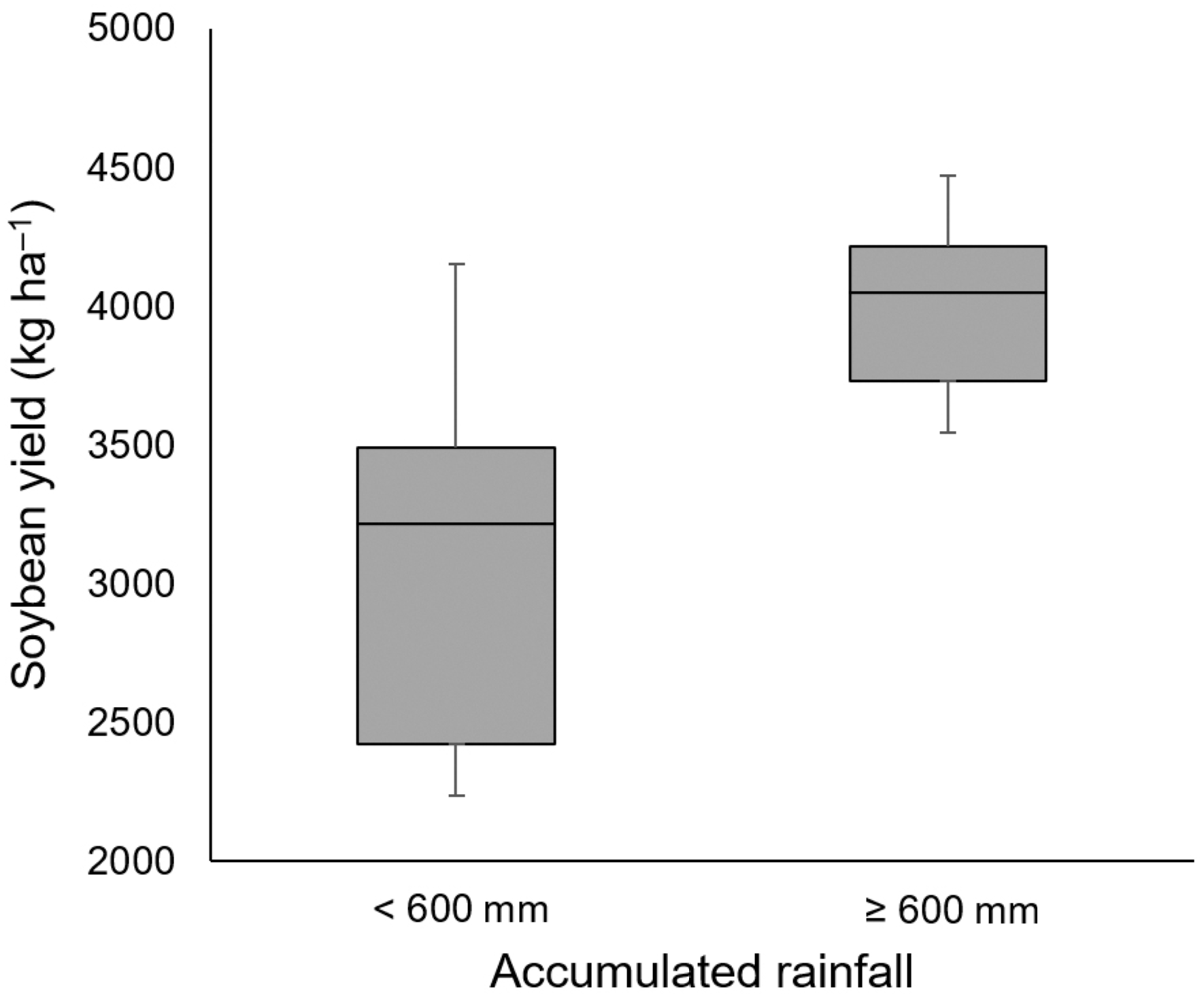
Why should space-time variability of rainfall be considered in precision agriculture for soybean in Piracicaba, São Paulo state?

ABSTRACT

Brazil ranks among the world's largest soybean producers; however, significant gaps in crop yield still exist, primarily linked to weather conditions. This study quantifies rainfall spatial variability using two dense networks of rain gauges and examines the impact of this variability on soybean crops’ attainable productivity. The study was carried out in Piracicaba, São Paulo state, Brazil. The first rain gauge network measuring campaign was conducted from 1993 to 1994, featuring ten gauges distributed in 1000 ha. The second rain gauge network was active from 2016 to 2018, comprising nine gauges covering 36 ha. A multi-model simulation was employed to assess the effect of rainfall spatial variability on soybean yield. The relative yield loss (Yg) due to water deficiency was simulated for three different sowing dates and across each rainfall sampling point. The findings indicate that the rainfall spatial variability directly influences attainable productivity. The extent of rainfall variability does not translate directly into yield outcomes; however, temporal variability associated with different sowing times significantly impacts soybean yield.

Keywords:
agro-climatic modeling; soybean yield; spatial variability; water management

Introduction

Brazilian farmers have adopted precision agriculture to map crop yields, which often show variability across many regions (Bottega et al., 2017). This variability arises from the complex interplay of numerous factors. Although advancements have been made in techniques for studying soil, plant, and phytosanitary management (Cherubin et al., 2022), the analysis of meteorological elements, particularly rainfall, remains insufficiently explored (Keswani et al., 2019; Mancipe-Castro and Gutiérrez-Carvajal, 2022).

Meteorological radars play a crucial role in assessing the temporal and spatial variability of rainfall, providing high-resolution data and near real-time localization of rain, particularly from convective systems (Lenzi et al., 1990; Venäläinen and Heikinheimo, 2002). However, in Brazil, the agricultural application of such data is limited due to availability constraints. Satellite products offer a viable alternative, but have coarser spatial resolution (Kidd and Levizzani, 2022). However, when combined with models, these satellite products can enhance our understanding of crop yield gaps (Lobell, 2013).

Notwithstanding the challenges posed by limited data availability, Brazilian farmers are increasingly turning to pluviometer grids to quantify rainfall and identify spatial variability. This method has been expanding due to enhanced rural connectivity and the proliferation of sensors and platforms (Pierce and Elliott, 2008; Jayaraman et al., 2016). Research employing these grids has effectively detected rainfall variability, particularly from convective systems, and highlighted environmental factors contributing to irregularity (Reichardt et al., 1995; Camargo et al., 2005; Silva et al., 2022a).

Rainfall measurements from farm-level networks have improved yield gap analysis when paired with crop models, enabling a more precise differentiation between meteorological influences and management practices (Lobell et al., 2015; Boote et al., 2003). In this sense, this study aimed to conduct an agrometeorological analysis of rainfall variability and its effects on soybean yield, employing two pluviometer grids that cover areas of 1000 ha and 36 ha.

Materials and Methods

Experimental site

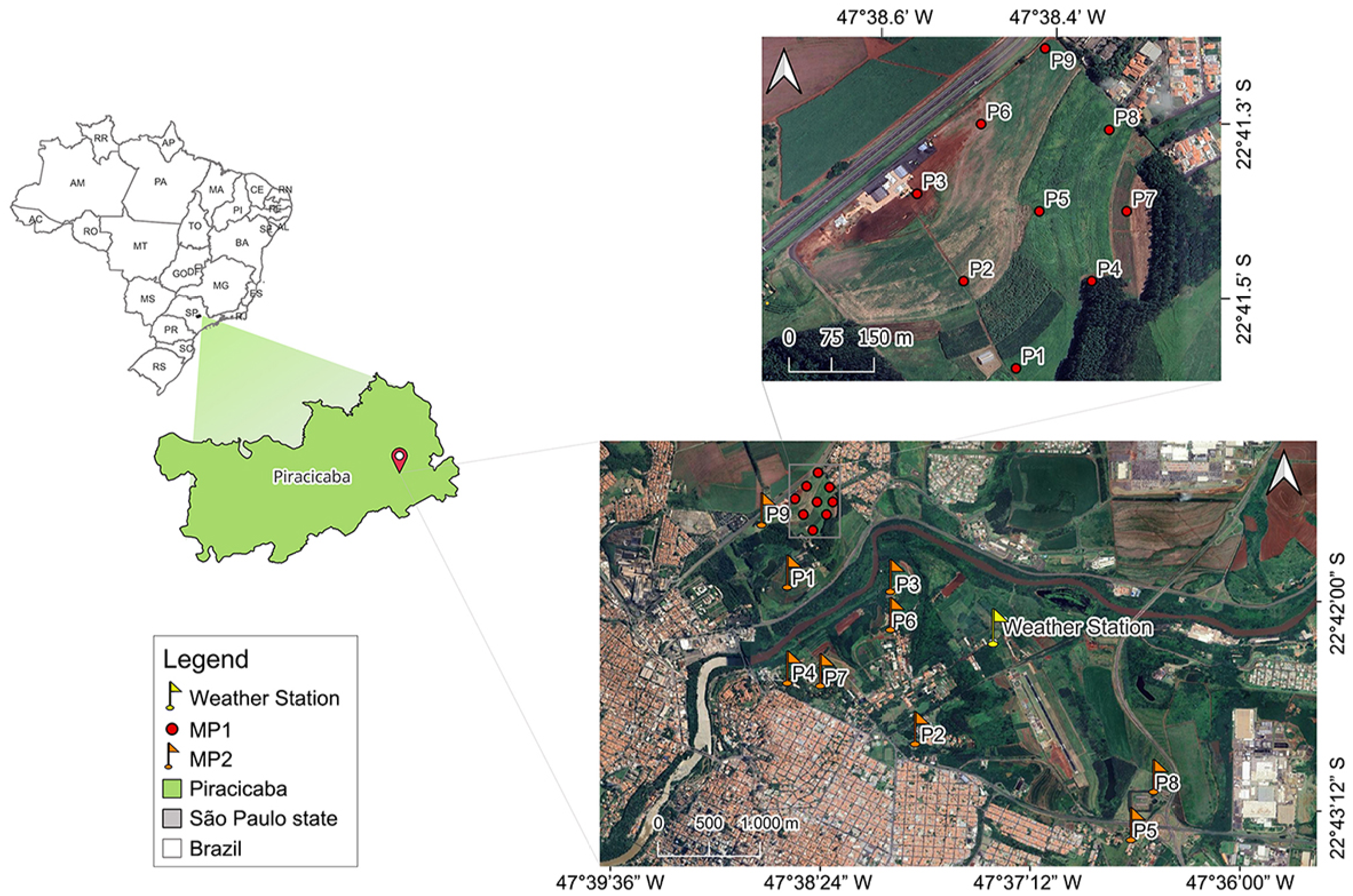
Data from two pluviometry grids were analyzed to assess rainfall variability (Figure 1, Table 1). The first pluviometry grid (MP1) was established by Reichardt et al. (1995) in 1993. It was designed to measure daily rainfall variability on a local scale of 1000 ha. The second pluviometry grid (MP2) was installed in 2016 to capture rainfall variability in a more localized area of 36 ha. Both pluviometry grids, MP1 and MP2, were situated in the municipality of Piracicaba, state of São Paulo, Brazil, within an area belonging to the Universidade de São Paulo, Escola Superior de Agricultura Luiz de Queiroz (USP/ESALQ).

Figure 1
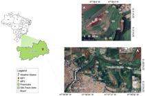
Location of the study site in the municipality of Piracicaba, São Paulo state, Brazil, and position of both pluviometry grids (MP1 and MP2) at the campus of the Universidade de São Paulo/Escola Superior de Agricultura Luiz de Queiroz. P1, P2, …, Pn refers the location of each rain gauge. MP1 = first pluviometry grid; MP2 = second pluviometry grid.

Table 1
Geographic position (latitude and longitude) of each rain gauge in the first and second pluviometry grids (MP1 and MP2). The coordinates were determined using Global Navigation Satellite System signal receivers (Garmin, model GPSMap 62s) and are provided in degrees, minutes, and seconds, with the WGS 84 system employed as the spatial reference.

MP1 Rain gauge	Latitude	Longitude	MP2 Rain gauge	Latitude	Longitude
P1	22°41’54.06" S	47°38’34.44" W	P1	22°41’35.52" S	47°38’26.52" W
P2	22°42’48.60" S	47°37’50.16" W	P2	22°41’30.12" S	47°38’29.76" W
P3	22°41’56.76" S	47°37’58.44" W	P3	22°41’24.72" S	47°38’32.64" W
P4	22°42’27.36" S	47°38’34.08" W	P4	22°41’30.12" S	47°38’21.84" W
P5	22°43’21.36" S	47°36’37.08" W	P5	22°41’25.80" S	47°38’25.08" W
P6	22°42’09.36" S	47°37’59.88" W	P6	22°41’20.40" S	47°38’28.68" W
P7	22°42’28.80" S	47°38’23.28" W	P7	22°41’25.80" S	47°38’19.68" W
P8	22°43’05.16" S	47°36’29.52" W	P8	22°41’20.76" S	47°38’20.76" W
P9	22°41’31.20" S	47°38’41.64" W	P9	22°41’15.72" S	47°38’24.72" W

The region's climate is classified as Cwa (Köppen classification), humid tropical, with rains concentrated between Oct and Mar and a dry period in autumn-winter (Alvares et al., 2013). According to historical data, annual rainfall averages 1350 mm.

Rain gauges

The nine pluviometers that comprised the MP1 (Reichardt et al., 1995) were randomly distributed across the USP/ESALQ area (Table 1). The shortest distance between the measurement points was 640 m, while the longest was 4406 m.

Rainfall measurements were collected daily from Nov 1993 to Oct 1994, totaling 364 days of data. The equipment used was manual, with a collection area of 300 cm² and an accuracy of 0.1 mm. The rain gauges were positioned 1.5 m above the ground surface, leveled, and unobstructed within a radius of at least 20 m. Additionally, a tenth collection point was the pluviometer located at the USP/ESALQ weather station (22°42’10" S, 47°37’24" W, altitude 546 m) (Figure 1).

In the experimental area of USP/ESALQ, known as "Fazenda Areão", the MP2 was installed. Nine rain gauges were positioned at approximately 200 m apart in a square grid layout, except P7 (Figure 1, Table 1). Data collection for this grid occurred from 08 Nov 2016 to 22 Jan 2018. Additionally, a tenth rain gauge was installed at the USP/ESALQ weather station, located 2250 m from the center of MP2. The minimum and maximum distances between pairs of MP2 rain gauges were 157 and 612 m, respectively.

The MP2 rain gauges utilized the "tipping bucket" design (Vaisala) and featured a collection area of 380 cm². They were installed at a height of 1.5 m above ground, calibrated beforehand, and leveled before being linked to data acquisition systems (Log Chart II) that recorded measurements every minute. The data were aggregated daily to facilitate analysis, generating daily totals from the minute-by-minute recordings.

Rainfall data analysis

The rainfall data from MP1 (Reichardt et al., 1995) and MP2 were evaluated to identify erroneous data and measurement failures. Since the grids were composed of nine pluviometers, along with the pluviometers installed at the Weather Station of USP/ESALQ (MP1 and MP2), it was possible to estimate the uncertainty of the measurements of each instrument based on the deviations from the average obtained from the pluviometers in operation. A validation method was also applied to identify erroneous data (Estévez et al., 2011). The analysis was based on the consistency test called the "range test" (Eq. 1).

(1) $$0\le P\le P_{MAX}$$

where P is the daily rainfall (mm) measured by each rain gauge, and P_MAX is the maximum daily rainfall value from historical data for Piracicaba, São Paulo state, Brazil.

Soybean yield models and simulation

To minimize uncertainties in the simulations, a variety of modeling approaches was employed (Asseng et al., 2013; Martre et al., 2015). The calibration of the crop models was previously conducted by Battisti et al. (2017), with additional details about the calibration process available in their study. Briefly, the calibration was carried out in three phases. The first phase was designed to assess the accuracy of simulations without any prior calibration. This was done using observed data on weather, soil profiles, and management practices such as sowing date, irrigation, fertilization, and initial conditions, with a cultivar like BRS 284 pre-loaded in the model. The second phase involved calibrating coefficients related to crop phenology, encompassing key growth stages such as emergence, flowering initiation, pod formation, seed development, and maturity. In the third phase, crop growth coefficients were calibrated above and below the soil surface. Optimal calibration was achieved by reducing the differences between simulated and observed values for yield, total dry matter, leaf area index, and harvest index.

Based on the agroecological zone models (Doorenbos and Kassam, 1979), the nitrogen and carbon model in agro-ecosystems v. 2.11 known as MONICA (Nendel et al., 2011) and the Crop System Model Soybean v. 4.6.1 provided in the Decision Support System for Agrotechnology Transfer platform (Boote et al., 1998, 2003; Jones et al., 2003) - which were previously calibrated and validated for the Piracicaba region, São Paulo state (Battisti et al., 2017), the potential yield (PP, kg ha^–1), attainable yield (PA, kg ha^–1) and relative yield loss (Yg, in %) were estimated (Eq. 2), considering water as the only limiting factor in the simulation.

The models required various meteorological inputs, including air temperature and humidity, wind speed, and solar radiation, which were obtained from the USP/ESALQ weather station. These inputs were treated uniformly across all simulation points for the same date. Although these factors can vary spatially due to rainfall patterns (Lobell et al., 2015), such variations were regarded as negligible considering the scale of the study areas (1000 ha and 36 ha). However, the data did differ across various sowing dates.

These simulations were carried out with complete mineral nutrition for the soybean crop in accordance with each model's specifications while integrating key agronomic parameters necessary for a realistic simulation of crop performance based on the conditions outlined by the respective modeling systems.

(2) $$Yg=(1-PA\text{/}PP)\times 100$$

The multi-model set was then obtained from the arithmetic mean of the yields simulated by the three models.

Simulations for the pluviometric meshes (MP1 and MP2) were carried out separately for each rainfall sample point within the grids (Figure 1). This method considered both spatial and temporal variability of rainfall. Specifically, three segments of rainfall data corresponding to each pluviometric mesh were analyzed, representing 130, 120, and 110 days from the sowing dates of 15 Nov, 15 Dec, and 15 Jan, as recommended by the Climatic Risk Zoning for Soybean Crop (MAPA, 2022). By conducting simulations for each sowing date at every rainfall sample point, it was possible to identify variations regarding sowing time and rainfall volume across the same agricultural production area, demonstrating the natural temporal and spatial precipitation variability.

The simulations were designed to evaluate the PP and PA of a GMR 6.5 cultivar, such as the cv. BRS 284 that was used to calibrate the models tested by Battisti et al. (2017).

An undisturbed soil sample collected at point (P4) of MP2 provided the soil water retention curve (van Genuchten, 1980). Assuming homogeneity in the soil across MP1 and MP2, we focused solely on the impact of rainfall on crop yield. The moisture levels were measured at field capacity (θcc), of 0.338 cm³ cm^–3 and at wilting point of 0.249 cm³ cm^–3, with the root system's maximum depth being 0.85 m. This resulted in the maximum soil water storage capacity (CAD) of 75 mm (Eq. 3).

(3) $$CAD=\left({\text{θ}}_{cc-}{\text{θ}}_{pmp}\right)z$$

Statistical analysis

Variability is expressed with the standard deviation and the coefficient of variation (CV). The CV expresses the standard deviation as a percentage of the mean. It measures the dispersion of the sample variables and is defined by Ayyub and McCuen (1997):

(4) $$CV=\frac{S}{\overline{X}}=\frac{\sqrt{\frac{1}{n-1}\left[{\displaystyle {\sum }_{i=1}^n{x}_i^2}-\frac{1}{n}{\left({\displaystyle {\sum }_{i-1}^n{x}_i}\right)}^2\right]}}{\frac{1}{n}{\displaystyle {\sum }_{i=1}^n{x}_i}}$$

where s is the standard deviation, which is the square root of the variance, $\overline{X}$ mean, and x_i sample and n is number of samples.

Results

Rainfall data for grids MP1 and MP2 were collected from nine sampling points over time and used to simulate soybean yield. The results from each of the nine locations demonstrate daily spatial variability in rainfall and temporal variability observed during the analyzed periods.

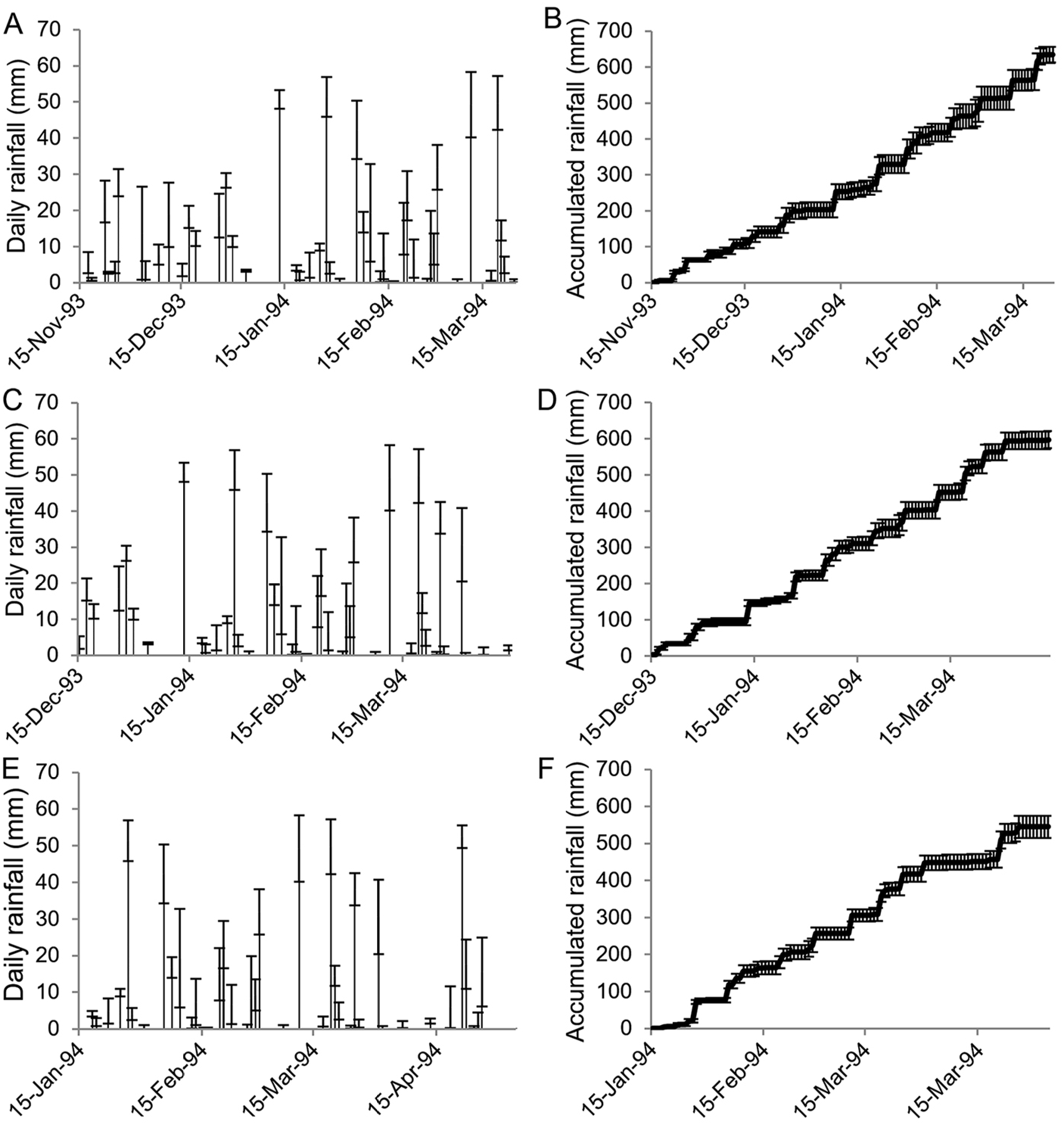
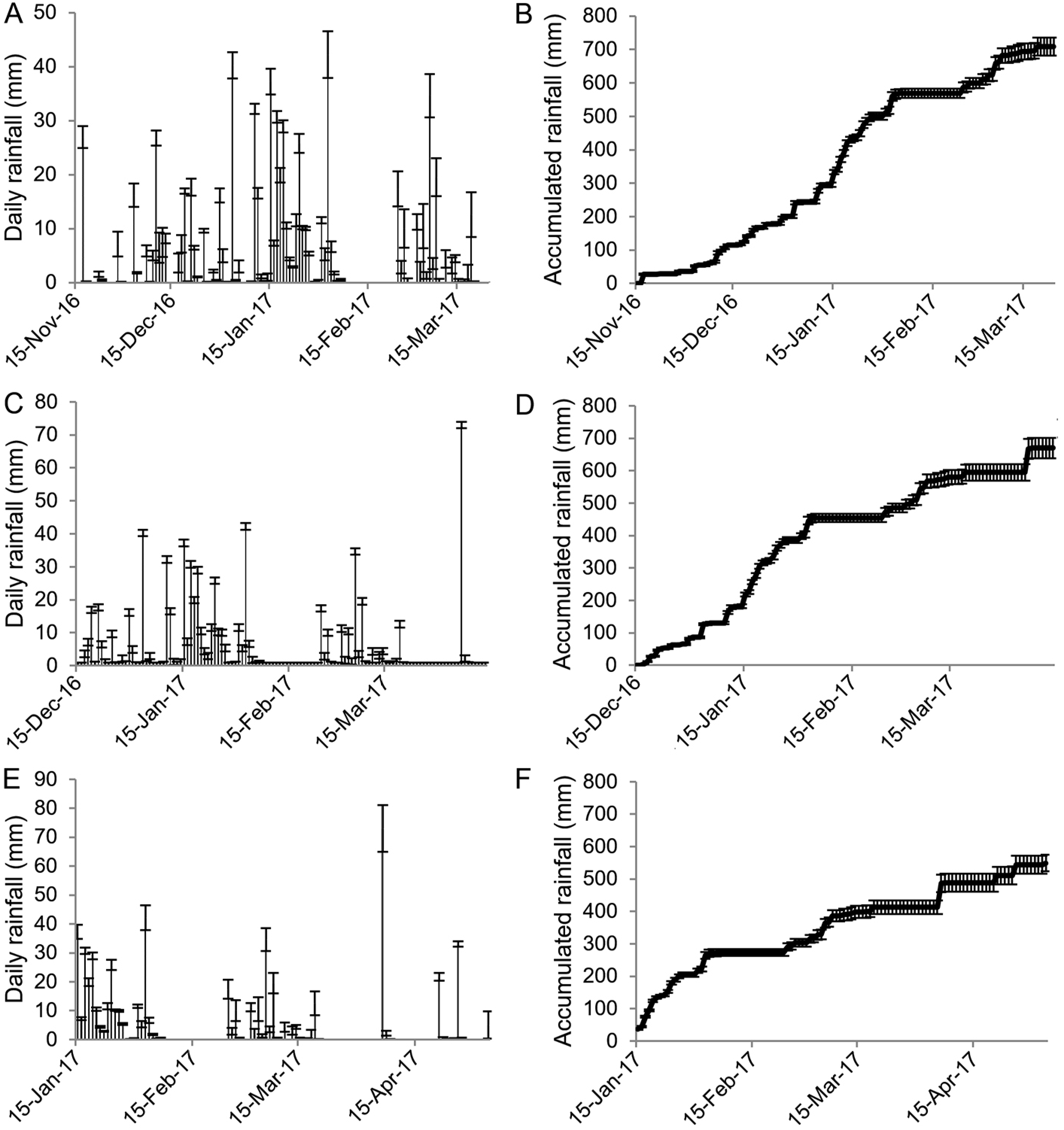
Three segments of rainfall data were selected from the rainfall data of MP1 and MP2, corresponding to measurement periods of 130, 120, and 110 days. These periods started on 15 Nov 1993 (MP1) or 2016 (MP2), 15 Dec 1993 (MP1) or 2016 (MP2) and 15 Jan 1994 (MP1) or 2017 (MP2). This analysis aimed to assess rainfall variability during the recommended periods for soybean cultivation in Piracicaba, São Paulo state, Brazil (Figures 2A-F and 3A-F).

Figure 2
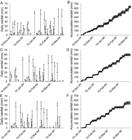
A, C, and E) Daily and B, D, and F) accumulated rainfall during the three series of the first pluviometry grid with 130, 120, and 110 days measured from 15 Nov 1993, 15 Dec 1993, and 15 Jan 1994, respectively, coinciding with the soybean production season in Piracicaba, São Paulo state.

Figure 3
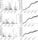
A, C, and E) Daily and B, D, and F) accumulated rainfall during the three series of the second pluviometry grid with 130, 120, and 110 days measured from 15 Nov 2016, 15 Dec 2016, and 15 Jan 2017, respectively, coinciding with the soybean production seasons in Piracicaba, São Paulo state.

Regarding MP1, the initial data collected from 15 Nov 1993 to 24 Mar 1994 showed 46 rainy days, which included 20 days with over 10 mm d^–1 (Figure 2A). The total rainfall over the 130-day period amounted to an average of 634.6 mm (Figure 2B). An analysis of the rainfall spatial variability from each MP1 rain gauge during this period indicated an average standard deviation of 3.77 mm d^–1, peaking at 13.5 mm d^–1. Furthermore, a temporal increase in standard deviation was observed when examining the cumulative rainfall across the sampling grid and assessing the differences between measurement points. By the study's conclusion, this value had risen to 22.3 mm, accounting for roughly 5 % of the water needs for soybean cultivation in the area (Silva et al., 2022b).

In the second analyzed MP1 series, from 15 Dec 1993 to 13 Apr 1994, there were 42 days of rainfall, four fewer than in the first season, even though this series had ten fewer total days (Figure 2C). Of these days, 18 experienced at least 10 mm of rainfall daily. The average accumulated rainfall for this series was 597.3 mm (Figure 2D), which is 37.3 mm lower than the first series. Regarding spatial variability, the mean standard deviation over the 120 evaluated days was 3.6 mm d^–1. On 09 Feb 1994, the maximum standard deviation reached 13.5 mm d^–1, linked to a daily rainfall of 19.3 mm d^–1, while the minimum was recorded at 1.3 mm d^–1 (P9) and the maximum at 31.8 mm d^–1 (P6). By the end of the second series (120 days), the standard deviation from the nine rain gauges measured 24 mm (Figure 2D), closely matching the value from the first series (Figure 2B).

The third series of MP1 rainfall data covered 110 days from 15 Jan 1994 (Figure 2E) and recorded 40 days of rain. Remarkably, on 15 of these days, the rainfall accumulated to at least 10 mm d^–1. The average accumulated rainfall recorded by the nine pluviometers in the MP1 grid was 544.8 mm (Figure 2F), which shows decreases of 14.2 and 8.8 % compared to the first (Figure 2B) and second (Figure 2D) series, respectively. This underscores the temporal differences among the three series. Over the 110 days, the average standard deviation across measurement points was 4 mm d^–1, with the maximum CV peaking at 13.5 mm d^–1 (Figure 2E). In terms of timing, the standard deviation of total rainfall at each point throughout this period was 29.7 mm (Figure 2F), reinforcing the evidence of spatial variability and its likely influence on the simulated soybean yield at each measurement point.

The MP2 data reveals rainfall spatial and temporal variability coinciding with soybean production phases in Piracicaba, São Paulo state (Figure 3A-F). This demonstrates a significant variation in distribution, with apparent differences noted among grades.

The first series of MP2, which lasted 130 days from 15 Nov 2016 to 14 Mar 2017, recorded 80 days of rain, including 27 days with over 10 mm d^–1 (Figure 3A). The total rainfall volume reached 708.7 mm (Figure 3B). An assessment of the rainfall spatial variability data over these 130 days showed a mean grid standard deviation of 1.1 mm d^–1, with the maximum standard deviation value relatively low at 4.3 mm d^–1 (Figure 3A). Furthermore, when analyzing the accumulated rainfall from each pluviometer and calculating the differences between measurement points, there was a temporal rise in the standard deviation, which increased to 26.6 mm by the end of this 130-day series (Figure 3B).

The second series of measurements (Figure 3C), taken over 120 consecutive days beginning on 15 Dec 2016, recorded 68 days of rain, 12 days fewer than the first MP2 series (Figure 3A), during which accumulated rain reached or surpassed 10 mm d^–1 on 25 days. The average rainfall accumulated by the grid during these 120 days totaled 669.8 mm (Figure 3D), 38.9 mm lower than the average in the first series (Figure 3B), which spanned 130 days. Regarding differences between rain gauges, which characterize rainfall spatial variability, the average standard deviation recorded over the 120 days was 1.2 mm d^–1 (Figure 3C). The maximum standard deviation value of this second MP2 data series was 8.1 mm d^–1, recorded on 06 Apr 2017, when the average rainfall accumulated by the grid reached 79.3 mm d^–1, twice the maximum standard deviation recorded for the first series (Figure 3A). After the 120-day measurement period, the standard deviation for the total rainfall accumulated reached 31.4 mm (Figure 3D), surpassing the temporal differences observed in the first series (Figure 3B). This emphasizes the probable spatial variability in yields resulting from meteorological factors, notably rainfall.

Although the average accumulated rainfall difference between the first two MP2 series (Figure 3B and D) was small at 5.5 %, the temporal distributions showed notable variations. This highlights the considerable influence that meteorological factors can exert on production activities at different times of the year, even within the same region.

During the 110-day analysis of the third MP2 series (Figure 3E), from 15 Jan to 04 May 2017, 53 days of rain were recorded, including 21 days with at least 10 mm d^–1 of rainfall. The total average rainfall measured by the nine pluviometers in the MP2 grid reached 549.4 mm (Figure 3F), showing a decline of 22.4 % from the first series (Figure 3B) and 18 % from the second series (Figure 3D). The rainfall spatial variability over these 110 days resulted in an average standard deviation of 1.38 mm d^–1, with a maximum value of 8 mm d^–1 (Figure 3E). Over the same period, the temporal standard deviation for the accumulated rainfall at each measurement point was 24.9 mm (Figure 3F).

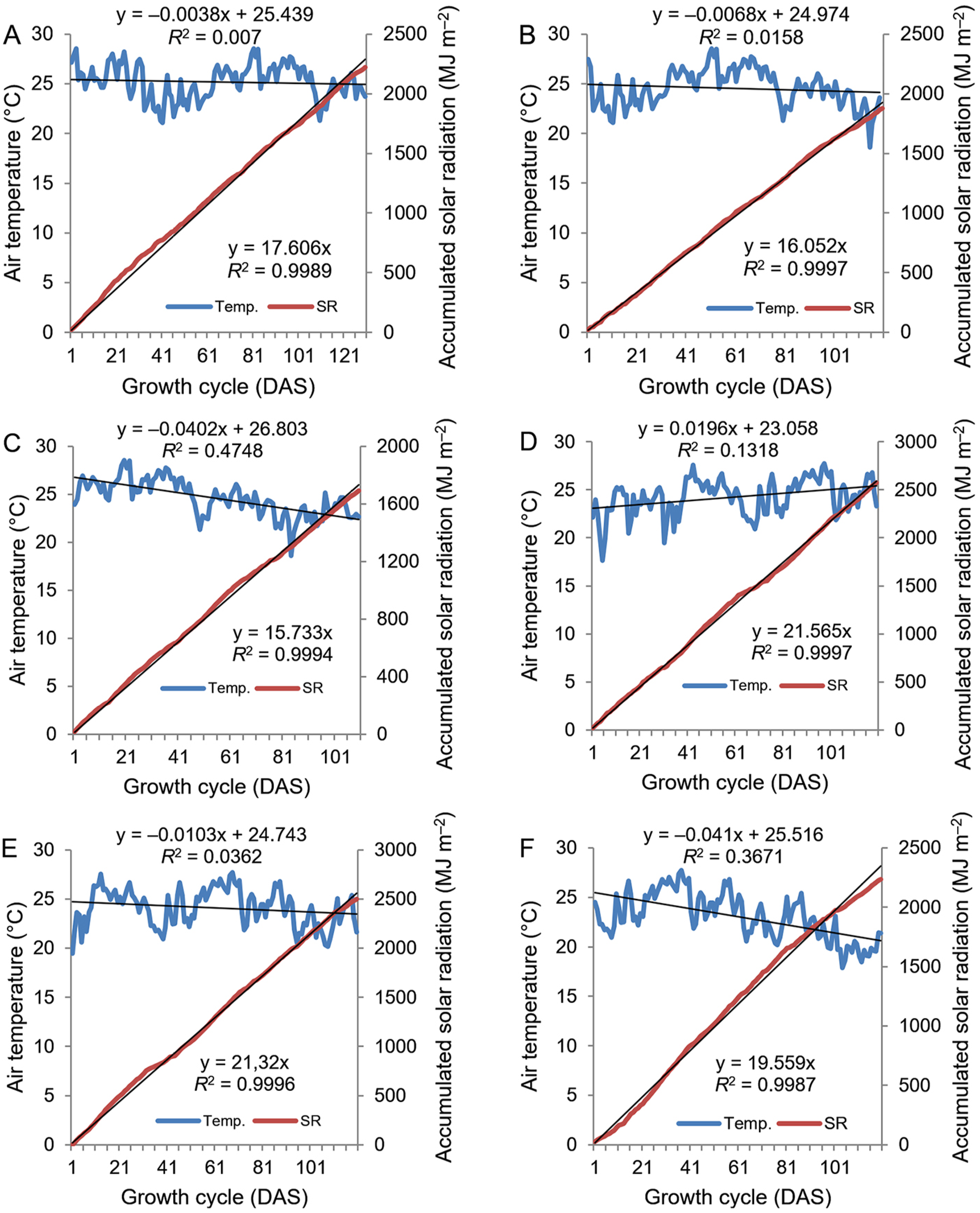
In addition to rainfall, air temperature and global solar radiation (SR) were assessed regarding the soybean production period (Figure 4A-F). However, unlike rainfall, measured individually at each of the nine points of MP1 (Figure 2A-F) and MP2 (Figure 3A-F), the variability of these two meteorological factors was not quantified within the grids. Instead, only daily data for each grid was available (Figure 4A-F).

Figure 4
Mean air temperature and global solar radiation (SR) accumulated over the series related to soybean production cycles of first pluviometry grid, measured from A) 15 Nov 1993, B) 15 Dec 1993, C) 15 Jan 1994 and second pluviometry grid, measured from D) 15 Nov 2016, E) 15 Dec 2016, and F) 15 Jan 2017. DAS = days after sowing; Temp. = daily mean air temperature.

The average air temperature showed minimal differences across the three data series pertaining to theoretical cycles of soybean production (Figure 4A-F). In the first MP1 series (Figure 4A), the average temperature was 24.2 °C, reflecting a slight downward trend. The second data series from the same grid (Figure 4B) displayed thermal conditions very similar to the first (Figure 4A), with an average temperature of 24.5 °C and a trend toward thermal decline, although slightly higher than that registered in the first series. The average temperature in the third series was 24.3 °C (Figure 4C), aligning closely with the previous series (Figure 4A and B). However, the delay in sowing for this series led to a more pronounced thermal decline of –0.04 °C d^–1.

Global solar radiation, crucial for plant growth and development, showed differing cumulative values across each series. For the MP1 data, the SR in the first series was 2177.3 MJ m^–2 (Figure 4A), while the second series recorded 2058.6 MJ m^–2 (Figure 4B) and the third series totaled 1952.4 MJ m^–2 (Figure 4C). The difference between successive cycles was approximately 5 %, leading to an overall reduction in radiant energy of 10.33 % from the first to the third series.

In the first series for MP2, the average air temperature was 24.2 °C (Figure 4D), indicating a positive trend throughout the cycle. Conversely, the second (Figure 4E) and third (Figure 4F) series showed a declining trend in average air temperature, with average values of 24.1 and 23 °C, respectively.

Regarding MP2, the SR in the first (Figure 4D) and second (Figure 4E) series was relatively comparable, with 2573.3 and 2502.1 MJ m^–2 values, respectively. In contrast, the third series, despite the lower rainfall volume (Figure 3E and F) and, therefore, probably a longer period of clear sky, the reduction of the photoperiod and consequently the SR resulted in 2233.1 MJ m^–2 (Figure 4F). Notably, this resulted in a decrease of approximately 12 % in radiant energy compared to the previous two series.

Values for PP (kg ha^–1), PA (kg ha^–1), and Yg (%) for the two areas, 1000 ha (MP1) and 36 ha (MP2), were calculated based on the set of models, as recommended by Asseng et al. (2013) and Martre et al. (2015) (Tables 2 and 3). Simulations were conducted separately for the nine rainfall measurement points within the MP1 and MP2 grids (Figure 1, Table 1). This method focused on the effect of rainfall variability on soybean PA and Yg. As a result, the soil in both areas was considered homogeneous regarding CAD. This aspect might affect the simulations by increasing or decreasing crop yield data deviations, regardless of rainfall.

Table 2
Accumulated rainfall (AC), attainable yield (PA), and relative yield loss (Yg) simulated for soybean for each point of the first pluviometry grid. Theoretical sowing dates: 15 Nov 1993, 15 Dec 1993 and 15 Jan 1994. Grouping results of the agroecological zone, the model for nitrogen and carbon in agro-ecosystems and the crop system model - soybean Decision Support System for Agrotechnology Transfer models.

Point	15 Nov 1993			15 Dec 1993			15 Jan 1994
	AC	PA	Yg	AC	PA	Yg	AC	PA	Yg
	mm	kg ha–1	%	mm	kg ha–1	%	mm	kg ha–1	%
P1	605.2	3752.2	33.6	583.4	3927.0	26.2	534.9	3250.5	29.2
P2	628.1	4101.9	27.5	566.1	4151.5	22.0	495.4	3277.2	28.7
P3	616.1	3951.6	30.1	595.8	3982.9	25.1	564.1	3372.4	26.6
P4	623.9	3908.9	30.9	571.6	3846.3	27.7	525.0	3036.1	33.9
P5	660.3	4000.3	29.3	599.4	3924.3	26.2	532.8	3180.6	30.8
P6	645.6	4067.3	28.1	615.4	4076.1	23.4	571.7	3324.3	27.6
P7	645.8	4006.5	29.1	617.1	4048.6	23.9	554.3	3208.8	30.2
P8	671.0	4043.0	28.5	641.2	4309.6	19.0	595.7	3488.4	24.1
P9	615.3	3728.7	34.1	585.8	3787.2	28.8	529.5	3215.6	30.0
Mean	634.6	3951.2	30.1	597.3	4005.9	24.7	544.8	3261.5	29.0
s	22.3	132.8	2.3	24.0	160.8	3.0	29.8	127.6	2.8
CV	3.5	3.4	7.8	4.0	4.0	12.2	5.5	3.9	9.6

• s = standard variation; CV= coefficient of variation (%).

Table 3
Accumulated rainfall (AC), attainable yield (PA), and relative yield loss (Yg) simulated for soybean for each point of the second pluviometry grid. Theoretical sowing dates: 15 Nov 2016, 15 Dec 2016 and 15 Jan 2017. Grouping results of the agroecological zone, the model for nitrogen and carbon in agro-ecosystems and the crop system model – soybean Decision Support System for Agrotechnology Transfer models.

Point	15 Nov 2016			15 Dec 2016			15 Jan 2017
	AC	PA	Yg	AC	PA	Yg	AC	PA	Yg
	mm	kg ha–1	%	mm	kg ha–1	%	mm	kg ha–1	%
P1	701.4	4275.3	33.7	655.2	3712.3	37.9	524.3	2449.6	49.9
P2	742.5	4467.8	30.7	707.7	4116.3	31.2	592.1	2765.3	43.7
P3	695.7	4266.7	33.8	646.7	3673.2	38.3	516.2	2424.0	50.5
P4	673.2	4249.3	34.0	621.9	3624.9	39.1	500.9	2327.5	52.3
P5	698.3	4220.4	34.4	645.7	3606.4	39.4	529.9	2386.7	51.4
P6	702.7	4215.5	34.5	643.6	3583.4	39.7	521.5	2321.0	52.7
P7	688.7	4239.3	34.1	637.9	3544.2	40.4	517.2	2291.2	53.3
P8	699.2	4210.8	34.6	645.4	3558.7	40.1	526.8	2328.8	52.5
P9	651.1	4077.8	36.5	598.7	3392.4	42.9	483.8	2234.4	54.2
Mean	694.8	4247.0	34.0	644.8	3645.8	38.8	523.6	2392.0	51.2
s	24.5	101.0	1.5	29.1	198.3	3.2	29.5	154.9	3.1
CV	3.5	2.4	4.4	4.5	5.4	8.2	5.6	6.5	6.1

• s = standard variation; CV = coefficient of variation (%).

Regarding MP1, the simulations did not consider the spatial variability of air temperature and SR (Figure 4A-C). This led to applying the same daily data across all nine measurement points (Figure 1, Table 1). Consequently, the PP was influenced exclusively by the sowing dates. For the sowing date of 15 Nov 1993, the simulation showed a PP of 5654.3 kg ha^–1. The results revealed a decrease in PP with delayed soybean sowing, resulting in yields of 5320 kg ha^–1 and 4594.3 kg ha^–1 for simulations that started on 15 Dec 1993 and 15 Jan 1994, respectively.

In MP1, the PA, affected by water availability, displayed rainfall spatial variability among the nine measurement points of MP1 (Figure 2A-F, Table 2) throughout the three series. The PA data for simulated sowing on 15 Nov 1993 showed an average of 3951.2 kg ha^–1, with a standard deviation of 132.8 kg ha^–1. Similarly, variability in PA was observed for the other two sowing dates: 15 Dec 1993, recorded an average PA of 4005.9 (± 160.8) kg ha^–1, while 15 Jan 1994 indicated an average of 3261.5 (± 127.6) kg ha^–1.

The yield from the sowing on 15 Dec 1993 exceeded that of previous sowings, even with a shorter growth cycle and lower potential yield (Table 2). This enhancement is linked to improved water conditions due to the temporal distribution of rainfall (Figure 2C and D, Table 2), which coincided with key stages of reproductive development during this second series.

In the simulated cycle beginning on 15 Nov 1993, the average Yg was 30.1 %, with a standard deviation of 2.3 % across the nine measurement points of MP1 (Table 2). Throughout this first series, the average rainfall measured was 634.6 mm, with a standard deviation of 22.3 mm (Figure 2B, Table 2). Examining the CV reveals that the yield variability, with a CV of 3.4 %, closely matched the rainfall variability, which had a CV of 3.5 %.

In the third production cycle of MP1, the Yg ranged between the first two cycles, with an average of 29 % (Table 2). The standard deviation of rainfall was higher at 29.8 mm, and the CV was 5.5 %. However, these metrics exceeded those recorded during the first two production cycles (Figure 2B and D). Importantly, the CV of PA was only 3.9 %, indicating that it was not the highest (Table 2). This finding underscores the absence of a direct relationship between accumulated rainfall and PA for a specific production cycle. Despite increased variability, the effects of dry spells depend on the crop's phenological stage, with varying intensity based on the plant's vulnerability to water stress.

Similarly, the simulations based on MP2 data (Table 3) failed to consider spatial variability in air temperature and SR (Figure 4D-F). The models projected PP of 6366, 5964.7, and 4942 kg ha^–1 for the planting dates on 15 Nov 2016, 15 Dec 2016, and 15 Jan 2017, respectively.

The average attainable yield (PA) of the three models (Table 3) revealed how meteorological factors can contribute to yield variability within production areas (O’Neal et al., 2002). For the first series, which involved sowing on 15 Nov 2016, the mean PA was recorded at 4247 kg ha^–1, with a standard deviation of 101 kg ha^–1. For the other two series analyzed, the results exhibited a similar trend, with PA values of 3645.8 (± 198.3) kg ha^–1 for the second series and 2392 (± 154.9) kg ha^–1 for the third series (Table 3).

The Yg related to water availability for MP2 (Table 3) consistently surpassed that of MP1 (Table 2) for all sowing dates. For the first sowing date on 15 Nov, the grid loss for MP2 was 34 %, which increased to 38.8 and 51.2 % for the simulated sowing dates on 15 Dec 2016, and 15 Jan 2017, respectively (Table 3). Although cycle length decreased with later sowing, the decline in accumulated rainfall, which correlated with reductions in cycle length and the subsequent temporal distribution across the production cycle (Figure 3A-F), resulted in the most substantial yield losses observed in MP2.

Discussion

The timing and volume of rainfall during the soybean growing season can vary substantially (Figures 2A-F and 3A-F), which affects crop growth in various ways (Purcell and Specht, 2004; Grassini et al., 2015; Sentelhas et al., 2015; Zanon et al., 2016). Regarding MP1, the reductions in accumulated rainfall from the first to the third series were 5.9 % from the first to the second series and 14.1 % from the first to the third (Figure 2B, D and F), both of which were lower than the reductions of 7.7 % (130 to 120 days) and 15.4 % (130 to 110 days) observed over time. Similarly, the analysis of MP2 data showed a 5.5 % reduction in accumulated rainfall between the first (130 days) and second (120 days) series (Figure 3B and D), which was also smaller than the time-related reduction. Notably, for this pluviometry grid, the decrease in accumulated rainfall from the first to the third series (22.5 % from 130 to 110 days) was proportionally more significant than the reduction observed over time between these series.

A reduction in yield potential associated with sowing delay due to water deficiency has been documented for Piracicaba, São Paulo state, by Battisti and Sentelhas (2019) in a study considering successive soybean sowing dates. In the present study, the results presented in Figures 2A-F and 3A-F do not demonstrate a proportional reduction in accumulated rainfall throughout the examined data series. This highlights a limitation, as energy conditions affect crop evapotranspiration variations beyond temporal differences (Figure 4A-F). Furthermore, the differences observed among the measurement points in each grid (Figures 2A-F and 3A-F) are likely responsible for the considerable yield differences observed among these sites (Tables 2 and 3).

The average temperature values of the three series, which consist of the MP1 (Figure 4A-C) and MP2 (Figure 4D-F) grids favor the growth and development of soybean crops (Farias et al., 2009). Furthermore, no critical temperatures could negatively impact soybean growth and development.

The availability of radiant energy after delayed sowing (Figure 4A-F) and a shortened development cycle contribute to a reduced yield potential for soybean crops (PP). Specifically, the PP values decrease due to sowing delay, falling from 5654.3 to 4594.3 kg ha^–1 (MP1) and 6366 to 4942 kg ha^–1 (MP2). These results align with the PP values presented by Battisti et al. (2017) and Battisti and Sentelhas (2019) for Piracicaba, São Paulo State, in the same sowing period.

Delays in soybean sowing expose the plants to cooler air temperatures and diminished solar radiation (Figure 4A-F), especially during reproductive stages, as reported in a study conducted by Zanon et al. (2016) in Rio Grande do Sul state, Brazil, which explained the yield loss of 26 kg ha⁻¹ d⁻¹ for crops sown from 4 Nov, considering crops without water limitation.

After examining the attainable yield data from each sampling point in the two grids for the three productions series assessed (Tables 2 and 3), we emphasize that there is no direct link between the accumulated rainfall and the attainable yield in a soybean production cycle. Additionally, our results indicate that rainfall's spatial and temporal variability influences variations in soybean yield (Purcell and Specht, 2004; Grassini et al., 2015; Zanon et al., 2016).

However, this variability often diminishes as the total rainfall increases during the soybean growing season (Figure 5). Increased rainfall volumes more effectively satisfy the plants’ water needs (Silva et al., 2022b), thereby mitigating the impact of water stress on soybean yield.

Figure 5
Box plot of soybean yield under different amounts of accumulated rainfall during the growing season.

The variation in soybean yield becomes markedly more pronounced when rainfall falls below 600 mm (Figure 5). In such cases, yields fluctuate between roughly 2200 and 4200 kg ha^–1, with a median yield around 3200 kg ha^–1. The interquartile range (IQR) extends from 2500 to 3500 kg ha^–1, indicating a broader distribution of yield data and increased susceptibility to water stress. In contrast, when accumulated rainfall reaches 600 mm or more, the variability in soybean yield significantly reduces. Yields in this category range from approximately 3500 to 4500 kg ha^–1, with a median yield of around 4000 kg ha^–1. The IQR for this scenario is tighter, between 3800 and 4300 kg ha^–1, suggesting that adequate rainfall sufficiently fulfills the water requirements of soybean plants, leading to more stable yields.

The rainfall data gathered from the rain gauges in the study areas revealed notable spatial and temporal variability in rainfall across various simulated sowing dates and measurement points. This variability directly affected soybean yield, as the models indicated significant differences in potential yield results. The spatial variability observed in the MP1 and MP2 data highlighted how rainfall fluctuations impacted yields, with standard deviations reaching as high as 160 and 198 kg ha^–1, respectively. These results emphasize the need to recognize and consider rainfall spatial distribution in agricultural management, particularly in regions with extensive and diverse production areas. Furthermore, temporal variability was a crucial factor influencing soybean phenology, affecting crop development and its vulnerability to water stress.

This study effectively identified uncertainties related to rainfall homogeneity in hypothetical soybean production areas of 1000 and 36 ha, revealing the direct correlation between meteorological factors and yield variability. Simulations conducted across different sowing dates, in conjunction with yield models, revealed that rainfall spatial variability can significantly impact crop yields. These findings underscore the necessity for agricultural management strategies that consider average rainfall and its spatial and temporal distribution throughout the crop cycle.

• Declaration of use of AI Technologies
  The authors declare that no AI technologies were used in the development of this paper. All analyses and conclusions are based on traditional methods and entirely the authors’ work.

Data availability statement

Data will be made available upon request.

Acknowledgments

This research was supported by the Fundação de Amparo à Pesquisa do Estado de São Paulo (FAPESP), grant number: 2015/14497-0.

References

• Alvares CA, Stape JL, Sentelhas PC, Gonçalves JLM, Sparovek G. 2013. Köppen's climate classification map for Brazil. Meteorologische Zeitschrift 22: 711-728. https://doi.org/10.1127/0941-2948/2013/0507
  » https://doi.org/10.1127/0941-2948/2013/0507
• Asseng S, Ewert F, Rosenzweig C, Jones JW, Hatfield JL, Ruane AC, et al. 2013. Uncertainty in simulating wheat yields under climate change. Nature Climate Change 3: 827-832. https://doi.org/10.1038/nclimate1916
  » https://doi.org/10.1038/nclimate1916
• Ayyub B, McCuen R. 1997. Probability, Statics, and Reliability for Engineers. CRC Press, Boca Raton, FL, USA.
• Battisti R, Sentelhas PC, Boote KJ. 2017. Inter-comparison of performance of soybean crop simulation models and their ensemble in southern Brazil. Field Crops Research 200: 28-37. https://doi.org/10.1016/j.fcr.2016.10.004
  » https://doi.org/10.1016/j.fcr.2016.10.004
• Battisti R, Sentelhas PC. 2019. Characterizing Brazilian soybean-growing regions by water deficit patterns. Field Crops Research 240: 95-105. https://doi.org/10.1016/j.fcr.2019.06.007
  » https://doi.org/10.1016/j.fcr.2019.06.007
• Boote KJ, Jones JW, Hoogenboom G. 1998. Simulation of crop growth: CROPGRO model. In: Peart RM, Shoup WD. eds. Agricultural systems modeling and simulation. CRC Press, Boca Raton, FL, USA. https://doi.org/10.1201/9781482269765
  » https://doi.org/10.1201/9781482269765
• Boote KJ, Jones JW, Batchelor WD, Nafziger ED, Myers O. 2003. Genetic Coefficients in the CROPGRO-Soybean Model. Agronomy Journal 95: 32-51. https://doi.org/10.2134/agronj2003.3200
  » https://doi.org/10.2134/agronj2003.3200
• Bottega EL, Queiroz DM, Pinto FAC, Valente DSM, Souza CMA. 2017. Precision agriculture applied to soybean. Part III. Spatial and temporal variability of yield. Australian Journal of Crop Science 11: 799-805. https://doi.org/10.21475/ajcs.17.11.07.pne383
  » https://doi.org/10.21475/ajcs.17.11.07.pne383
• Camargo MBP, Brunini O, Pedro Junior MJ, Bardin L. 2005. Spatial and temporal variability of daily air temperature and precipitation data of the IAC weather station network, São Paulo State, Brazil. Bragantia 64: 473-483 (in Portuguese, with abstract in English). https://doi.org/10.1590/S0006-87052005000300018
  » https://doi.org/10.1590/S0006-87052005000300018
• Cherubin MR, Damian JM, Tavares TR, Trevisan RG, Colaço AF, Eitelwein MT, et al. 2022. Precision agriculture in Brazil: the trajectory of 25 years of scientific research. Agriculture 12: 1882. https://doi.org/10.3390/agriculture12111882
  » https://doi.org/10.3390/agriculture12111882
• Doorenbos J, Kassam AH. 1979. Yield Response to Water. FAO, Rome, Italy.
• Estévez J, Gavilán P, Giráldez JV. 2011. Guidelines on validation procedures for meteorological data from automatic weather stations. Journal of Hydrology 402: 144-154. https://doi.org/10.1016/j.jhydrol.2011.02.031
  » https://doi.org/10.1016/j.jhydrol.2011.02.031
• Farias JRB, Neumaier N, Nepomuceno AL. 2009. Soja. In: Monteiro JEBA. ed. Agrometeorologia dos cultivos: o fator meteorológico na produção agrícola. Instituto Nacional de Meteorologia, Brasília, DF, Brazil (in Portuguese).
• Grassini P, Torrion JA, Yang HS, Rees J, Andersen D, Cassman KG, et al. 2015. Soybean yield gaps and water productivity in the western U.S. corn belt. Field Crops Research 179: 150-163. https://doi.org/10.1016/j.fcr.2015.04.015
  » https://doi.org/10.1016/j.fcr.2015.04.015
• Jayaraman PP, Yavari A, Georgakopoulos D, Morshed A, Zaslavsky A. 2016. Internet of things platform for smart farming: experiences and lessons learnt. Sensors 16: 1884. https://doi.org/10.3390/s16111884
  » https://doi.org/10.3390/s16111884
• Jones JW, Hoogenboom G, Porter CH, Boote KJ, Batchelor WD, Hunt LA, et al. 2003. The DSSAT cropping system model. European Journal of Agronomy 18: 235-265. https://doi.org/10.1016/S1161-0301(02)00107-7
  » https://doi.org/10.1016/S1161-0301(02)00107-7
• Keswani B, Mohapatra AG, Mohanty A, Khanna A, Rodrigues JJPC, Gupta D, et al. 2019. Adapting weather conditions based IoT enabled smart irrigation technique in precision agriculture mechanisms. Neural Computing and Applications 31: 277-292. https://doi.org/10.1007/s00521-018-3737-1
  » https://doi.org/10.1007/s00521-018-3737-1
• Kidd C, Levizzani V. 2022. Satellite rainfall estimation. p. 135-170. In: Morbidelli R. ed. Rainfall modeling, measurement and applications. Elsevier, Amsterdam, The Netherlands. https://doi.org/10.1016/B978-0-12-822544-8.00005-6
  » https://doi.org/10.1016/B978-0-12-822544-8.00005-6
• Lenzi G, Nanni S, Salsi A. 1990. Agricultural use of weather radar data in Emilia-Romagna Italy. In: Collier CG, Chapuis M. eds. Weather radar networking. Springer, Dordrecht, The Netherlands. https://doi.org/10.1007/978-94-009-0551-1_57
  » https://doi.org/10.1007/978-94-009-0551-1_57
• Lobell DB. 2013. The use of satellite data for crop yield gap analysis. Field Crops Research 143: 56-64. https://doi.org/10.1016/j.fcr.2012.08.008
  » https://doi.org/10.1016/j.fcr.2012.08.008
• Lobell DB, Thau D, Seifert C, Engle E, Little B. 2015. A scalable satellite-based crop yield mapper. Remote Sensing of Environment 164: 324-333. https://doi.org/10.1016/j.rse.2015.04.021
  » https://doi.org/10.1016/j.rse.2015.04.021
• Mancipe-Castro L, Gutiérrez-Carvajal RE. 2022. Prediction of environment variables in precision agriculture using a sparse model as data fusion strategy. Information Processing in Agriculture 9: 171-183. https://doi.org/10.1016/j.inpa.2021.06.007
  » https://doi.org/10.1016/j.inpa.2021.06.007
• Martre P, Wallach D, Asseng S, Ewert F, Jones JW, Rötter RP, et al. 2015. Multimodel ensembles of wheat growth: many models are better than one. Global Change Biology 21: 911-925. https://doi.org/10.1111/gcb.12768
  » https://doi.org/10.1111/gcb.12768
• Ministério da Agricultura, Pecuária e Abastecimento [MAPA]. 2022. Zoneamento Agrícola. MAPA, Brasília, DF, Brazil (in Portuguese). Available at: https://mapa-indicadores.agricultura.gov.br/publico/extensions/Zarc/Zarc.html [Accessed Mar 15, 2022]
  » https://mapa-indicadores.agricultura.gov.br/publico/extensions/Zarc/Zarc.html
• Nendel C, Berg M, Kersebaum JC, Mirschel W, Specka X, Wegehenkel M, et al. 2011. The MONICA model: testing predictability for crop growth, soil moisture and nitrogen dynamics. Ecological Modelling 222: 1614-1625. https://doi.org/10.1016/j.ecolmodel.2011.02.018
  » https://doi.org/10.1016/j.ecolmodel.2011.02.018
• O’Neal MR, Frankenberger JR, Ess DR. 2002. Use of CERES-maize to study effect of spatial precipitation variability on yield. Agricultural Systems 73: 205-225. https://doi.org/10.1016/S0308-521X(01)00095-6
  » https://doi.org/10.1016/S0308-521X(01)00095-6
• Pierce FJ, Elliott TV. 2008. Regional and on-farm wireless sensor networks for agricultural systems in Eastern Washington. Computers and Electronics in Agriculture 61: 32-43. https://doi.org/10.1016/j.compag.2007.05.007
  » https://doi.org/10.1016/j.compag.2007.05.007
• Purcell LC, Specht JE. 2004. Physiological traits for ameliorating drought stress. In: Shibles RM, Harper JE, Wilson RF, Shoemaker RC. eds. Soybeans: improvement, production, and uses. SSSA, Madison, WI, USA. https://doi.org/10.2134/agronmonogr16.3ed.c12
  » https://doi.org/10.2134/agronmonogr16.3ed.c12
• Reichardt K, Angelocci LR, Bacchi OOS, Pilotto JE. 1995. Daily rainfall variability at a local scale (1,000 ha), in Piracicaba, SP, Brazil, and its implications on soil water recharge. Scientia Agricola 52: 43-49. https://doi.org/10.1590/S0103-90161995000100008
  » https://doi.org/10.1590/S0103-90161995000100008
• Sentelhas PC, Battisti R, Câmara GMS, Farias JRB, Hampf AC, Nendel C. 2015. The soybean yield gap in Brazil: magnitude, causes and possible solutions for sustainable production. Journal of Agricultural Science 153: 1394-1411. https://doi.org/10.1017/S0021859615000313
  » https://doi.org/10.1017/S0021859615000313
• Silva ASA, Barreto IDC, Cunha-Filho M, Menezes RSC, Stosic B, Stosic T. 2022a. Spatial and temporal variability of precipitation complexity in northeast Brazil. Sustainability 14: 13467. https://doi.org/10.3390/su142013467
  » https://doi.org/10.3390/su142013467
• Silva EHFM, Hoogenboom G, Boote KJ, Gonçalves AO, Marin FR. 2022b. Predicting soybean evapotranspiration and crop water productivity for a tropical environment using the CSM-CROPGRO-Soybean model. Agricultural and Forest Meteorology 323: 109075. https://doi.org/10.1016/j.agrformet.2022.109075
  » https://doi.org/10.1016/j.agrformet.2022.109075
• van Genuchten MT. 1980. A closed form equation for predicting the hydraulic conductivity of unsaturated soils. Soil Science Society of America Journal 44: 892-898. https://doi.org/10.2136/sssaj1980.03615995004400050002x
  » https://doi.org/10.2136/sssaj1980.03615995004400050002x
• Venäläinen A, Heikinheimo M. 2002. Meteorological data for agricultural applications. Physics and Chemistry of the Earth 27: 1045-1050. https://doi.org/10.1016/S1474-7065(02)00140-7
  » https://doi.org/10.1016/S1474-7065(02)00140-7
• Zanon AJ, Streck NA, Grassini P. 2016. Climate and management factors influence soybean yield potential in a subtropical environment. Agronomy Journal 108: 1447-1454. https://doi.org/10.2134/agronj2015.0535
  » https://doi.org/10.2134/agronj2015.0535

Edited by

• Edited by:
  Quirijn de Jong van Lier

Publication Dates

• Publication in this collection
  11 Aug 2025
• Date of issue
  2025

History

• Received
  16 Sept 2024
• Accepted
  24 Feb 2025