Gaussian process regression as an alternative to kriging and SVM for spatial yield prediction¹

ABSTRACT

Detecting spatial yield variability is essential for precision agriculture because it minimizes environmental impact and enhances economic returns. This study proposes Gaussian Process Regression (GPR) as a predictive model for yield estimation, particularly in cultivated areas where the highest yields appear in the central region of the field, while the edges exhibit lower productivity. The study was conducted in Patos de Minas, Brazil, using 795 georeferenced soybean yield samples over 3.7 hectares. The analysis evaluates GPR across different sample sizes and compares it with Ordinary Kriging (OK) and Support Vector Machine (SVM). The results indicate that GPR and OK perform similarly under high sampling densities, but GPR achieves higher predictive accuracy under low-sampling conditions. A sample size of at least 60% of the full dataset is necessary to maintain reliable spatial prediction, as smaller sample sizes lead to greater prediction errors and less defined spatial patterns. SVM, in contrast, produces a smoothing effect across all sampling densities, which reduces its ability to capture local variations. These findings highlight GPR as a robust alternative for yield mapping, particularly in scenarios with limited data availability. From a practical perspective, GPR and OK remain strong candidates for yield prediction, reinforcing the importance of model selection based on data availability and spatial variability.

Keywords
modeling; geostatistics; machine learning; interpolation; spatial analysis

INTRODUCTION

The accuracy of the spatial interpolation method used to generate soybean yield distribution maps directly influences their reliability. Methods such as OK and SVM provide different approaches to spatial data interpolation, each with specific data requirements and analytical complexity.

OK remains a widely used geostatistical approach that models spatial correlations through a semivariogram, based on the assumption that nearby points exhibit greater similarity than distant ones. While it provides unbiased estimates and allows for uncertainty quantification, its performance depends on a well-defined spatial structure and tends to decline with sparse data or when stationarity assumptions are violated.(¹) Alternatively, machine learning methods, such as SVM, can capture complex, nonlinear spatial relationships without requiring a predefined statistical model. However, their effectiveness depends on careful parameter tuning and the availability of a sufficiently large dataset, as performance tends to deteriorate when sample density is low.(²) Recent studies have compared geostatistical and machine learning approaches for spatial predictions in precision agriculture, emphasizing the importance of selecting appropriate interpolation methods.(³)

GPR represents a promising alternative for crop yield modeling, offering a nonparametric, kernel-based probabilistic framework that eliminates the need to assume a predefined functional relationship between variables. GPR has been extensively applied in agriculture to model nonstationary and nonlinear relationships. For example, Campos-Taberner et al.(⁴⁾ employed GPR to estimate the Leaf Area Index (LAI) from smartphone images, demonstrating its potential for precision agriculture. Similarly, Martínez-Ferrer et al.(⁵) applied GPR for crop yield estimation and interpretability, integrating multisensor satellite observations and meteorological data to represent complex spatial and temporal dynamics. Additionally, Alebele et al.(⁶) explored Gaussian Kernel Regression to estimate crop yield from combined optical and Synthetic Aperture Radar (SAR) imagery, reinforcing its effectiveness in agricultural monitoring. These studies highlight GPR’s capacity to handle sparse sampling scenarios and enhance yield prediction accuracy, positioning it as a robust tool for spatial interpolation in precision agriculture.

This study investigates the use of GPR to estimate and analyze the spatial variability of soybean yield. As a crop of significant global economic importance, soybean production requires an understanding of yield spatial variability to optimize input allocation and minimize the impacts of environmental and physiological factors on field performance.(⁷) Soybean yield depends on a combination of biotic and abiotic factors that directly influence its spatial distribution, posing challenges for accurate modeling.

To address these challenges, this study evaluates the accuracy of the GPR method under different sample sizes to determine the extent to which a reduction in sample density affects the quality of spatial estimates. Additionally, the performance of GPR is compared with SVM and OK, both implemented in the Smart-Map plugin integrated into QGIS.

MATERIAL AND METHODS

Study Area and Available Dataset

The data for this study were collected in the municipality of Patos de Minas, specifically in the Santana de Patos neighborhood (Figure 1). The study area is located at 18º 51’ 32”S latitude and 46º 29’ 49”W longitude, with an average elevation of approximately 832 m. The region's climate falls under the "Aw" category in Köppen’s climate classification system,(⁸) which corresponds to a humid subtropical or mild temperate climate. Additionally, the average temperature is 21.8 ºC, and the annual average precipitation is 1296 mm.(⁹)

Figure 1
Study area.

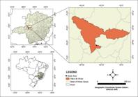
The study area covers approximately 3.7 hectares. Soybean seeds were planted in August 2022 and harvested in November 2022. Immediately after harvesting, the data were extracted from the grain harvester in “.csv” format and later converted into a shapefile format for processing.

The dataset is composed by 795 sampling points, characterized by yield mass, measured in tons per hectare (t/ha), and spatial location in Cartesian coordinates within the UTM projection system (E, N) – 23S zone. Yield data were obtained using a John Deere S440 combine harvester equipped with a factory-installed yield monitoring system. The monitor recorded yield at a rate of approximately one point per meter of harvester movement. Soybean rows were spaced 0.50 m apart, which is the standard row configuration commonly used in Brazilian soybean production. The spatial distribution of the samples is shown in Figure 2, with coordinates standardized using the z-score method to ensure a mean of 0 and a standard deviation of 1.

Figure 2
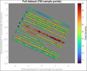
Spatial distribution of sampling points with yield variability in the field. (The gaps observed in some portions of the field, particularly within central rows, resulted from the removal of inconsistent yield readings. These included isolated zero-value measurements, sensor dropouts, and outlier points inherent to harvester-based yield monitoring systems. Such values were excluded during preprocessing to ensure the reliability of the spatial analysis).

According to Figure 2, the highest yield values are observed in the central region of the field (red circle), while the edges exhibit lower productivity (blue circle). This phenomenon is attributed to the border effect, which is common in cultivated areas where plants near the edges are more exposed to external factors such as microclimatic variations and pollutant contamination.

Gaussian Process Model for Soybeans Yield Estimation

GPR is a nonparametric Bayesian regression method that defines a distribution over possible functions that fit the observed data. GPR was employed here to model and predict soybean yield based on spatial data, we assume that the yield function follows a Gaussian Process (GP), meaning that the function values at any finite set of points follow a multivariate Gaussian distribution:

(1) $f\left(x\right) ~ GP\left[m\left(x\right),k(x,x\text{'})\right]$

where m(x) is the mean function (expectation):

(2) $m\left(x\right)=E\left[f\left(x\right)\right]$

$k\left(x,x\text{'}\right)$ is the covariance function (kernel):

(3) $$k\left(x,x\text{'}\right)=E\left[\left(f\left(x\right)-m\left(x\right)\right)\left(f(x\text{'})-m(x\text{'})\right)\right]$$

The kernel function defines spatial similarity between points, i.e., determines the smoothness and generalization of the predictions and can be fine-tuned to model different data patterns. A GP assumes that any finite subset of points x follows a multivariate Gaussian distribution. In this approach, the input variables x consisted of the cartesian coordinates (x,y) representing the spatial location of each sampling point, while the output variable f(x) corresponded to observed soybean yield values (t/ha).

The GPR Model can be then formulated as follows. Let’s start by considering that a training dataset is available as:

(4) $D={\left\{\left(x_i,y_i\right)\right\}}_i^N$

where:

(5) $y_i=f\left(x_i\right)+\epsilon ,\epsilon ~N\left(0,{\sigma }_i^2\right)$

GPR assumes that the data follows a joint Gaussian distribution:

(6) $y~N\left(m,K+{\sigma }^2{I}_n\right)$

where:

$y={\left[y_1,y_2,...,y_n\right]}^T$ is the observation vector composed by the yield values from training dataset; $m={\left[m\left(x_1\right),m\left(x_2\right),\dots ,m\left(x_n\right)\right]}^T$ is the mean vector; K is the covariance matrix, where $K_{ij}=k\left(x_i,x_j\right);{\sigma }^2{I}_n$; represents the uncertainty (noise) of the observations (I is the identity matrix by assuming the observations are independent).

For a new test point x_*, we want to estimate its output f_*. The joint distribution between the observed data and the new prediction is given by:

(7) $\left(\begin{array}{c}y\\ f_{*}\end{array}\right)~N\left(\left[\begin{array}{c}m\\ m_{*}\end{array}\right],\left[\begin{array}{cc}K+{\sigma }^2{I}_n& k_{*}\\ k_{*}^T& k\left(x_{*},x_{*}\right)\end{array}\right]\right)$

where $m_{*}=m\left(x_{*}\right)$ is the predicted mean and $k_{*}={\left[k\left(x_{*},x_1\right),...,k\left(x_{*},x_n\right)\right]}^T$ is the covariance between the new point and training data.

The conditional distribution of f_* given the observed data follows a Gaussian distribution:

(8) $f_{*}|x_{*},D~N\left({\mu }_{*},{\sigma }_{*}^2\right)$

where the predicted mean can be computed as:

(9) ${\mu }_{*}=m_{*}+k_{*}^T{\left(K+{\sigma }^2{I}_n\right)}^{-1}\left(y-m\right)$

and the variance as:

(10) ${\sigma }_{*}^2=k\left(x_{*},x_{*}\right)-k_{*}^T{\left(K+{\sigma }^2{I}_n\right)}^{-1}{K}_{*}$

The performance of GPR strongly depends on the choice of kernel function. In this study, the Rational Quadratic Kernel with a separate length scale per predictor was chosen due to its ability to handle multi-scale variations in spatial data, making it well-suited for yield prediction in heterogeneous fields. This approach has been shown to improve model generalization in environmental data applications by capturing both global and local variations in spatial relationships.(¹⁰)

The Rational Quadratic Kernel is given by:

(11) $k\left(x,x\text{'}\right)={\sigma }^2{\left(1+\frac{{||x-x\text{'}||}^2}{2\alpha l^2}\right)}^{-\alpha }$

where σ² is the variance parameter; ℓ is the length-scale parameter, adapted separately for each predictor (x,y); α is the scale-mixing parameter, controlling how much local variation is modeled; and x = (x, y) are spatial locations. More details about GPR can be found in Rasmussen and Williams.(¹¹) This model was trained according to experimental setup and subsequently applied to generate an interpolated yield map. Here, the hyperparameters σ², l, were optimized through Maximum Likelihood Estimation (MLE). All analyses involving GPR were performed using MATLAB software, employing the Statistics and Machine Learning Toolbox. The GPR models were implemented using the built-in “fitrgp” function, with hyperparameters optimized via MLE.

Experimental Setup

To ensure an unbiased evaluation, the dataset was randomly split into two subsets, namely the internal validation set in which 70% (557 sample points) of the data was used for k-fold cross-validation; and the external validation set which consisted of 30% (238 sample points) of the original dataset, excluded from the entire k-fold cross-validation process and only used for final performance assessment. The external validation set was used to simulate real operational conditions, assessing the model’s ability to generalize when new data becomes available. This realistic evaluation provides a more reliable estimate of the model’s predictive performance beyond the k-fold cross-validation process.(¹²)

The internal validation set (IVS) corresponds to 70% of the original dataset (557 sample points). The IVS (100%) represents the complete internal validation set and therefore does not correspond to the full dataset. The IVS was then randomly and uniformly subsampled into smaller subsets, namely 80% IVS (446 points), 60% IVS (334 points), 40% IVS (223 points), and 20% IVS (112 points), as displayed in Figure 3. This methodology allowed for an assessment of how reducing the number of observations impacts model performance while maintaining the statistical representativeness of the data.

Figure 3
Distribution of sampled points at different dataset sizes: (a) Full dataset available (795 points), (b) 100% IVS (557 points), (c) 80% IVS (446 points), (d) 60% IVS (334 points), (e) 40% IVS (223 points), and (f) 20% IVS (112 points). The color scale represents soybean yield (t/ha), illustrating the point-by-point of yield across different sampling densities.

Table 1 presents the mean, median, standard deviation (Std. Dev.), maximum (Max.), minimum (Min.), coefficient of variation (CV %), and Range for each sample size.

Table 1
Statistical summary of sample sizes

Sample Size	Mean(t/ha)	Median(t/ha)	Std. Dev. (t/ha)	Max(t/ha).	Min. (t/ha)	CV (%)	Range (t/ha)
Full dataset	4.89	4.77	1.26	8.94	0.60	25.66	8.34
557 points (IVS 100%)	4.93	4.79	1.28	8.94	0.60	26.06	8.34
446 points (IVS 80%)	4.93	4.80	1.26	8.85	0.60	25.66	8.24
334 points (IVS 60%)	4.93	4.75	1.29	8.85	1.60	26.27	7.24
223 points (IVS 40%)	4.88	4.72	1.30	8.85	1.60	26.74	7.24
112 points (IVS 20%)	4.83	4.59	1.30	8.85	1.60	26.93	7.24

The statistical analysis of the subsamples compared to the full dataset (795 sample points) indicates that their characteristics have been largely preserved (Table 1). The mean and median remain stable across the different subsamples, with only minor deviations. The largest difference is observed in the 20% IVS sample, where the median decreases by -1.05%. The standard deviation shows a slight increase in dispersion in smaller subsamples, reaching +3.17% in the 40% and 20% IVS samples.

Regarding the maximum and minimum values, the maximum yield remains nearly constant in the larger subsamples, but a slight reduction of -1.01% is observed in smaller subsets. In contrast, the minimum value increases significantly (+166.67%) from the 60% IVS sample onwards, suggesting that very low values were excluded from these subsets. The coefficient of variation (CV%) shows a gradual increase, reaching +4.21% in the 40% IVS sample, indicating a slight loss of homogeneity in smaller subsets.

The range, representing the difference between the maximum and minimum values, decreases progressively. This effect is noticeable from the 80% IVS sample (-1.20%) and becomes more pronounced in smaller subsets, with a reduction of -13.19% in the 60% and 40% IVS samples. This suggests that extreme values, particularly at the lower end, were removed in these cases.

Overall, the statistical characteristics of the subsamples remain closely aligned with those of the full dataset, confirming that they are well-representative of the original distribution. However, smaller subsets tend to exclude extreme values, particularly at the lower end of the yield range.

For each sample size scenario presented in Figure 3 and Table 1, the GPR model was internally validated using 5-fold cross-validation, following the common setting reported in the Smart-Map/QGIS workflow for Ordinary Kriging (OK) and Support Vector Machine (SVM).(¹³) Once trained within each scenario, the fitted model was applied to an external validation sample (30% of the full dataset, comprising 238 points) to assess its predictive performance in an independent dataset (Figure 4).

Figure 4
Distribution of the 238 out-of-sample points used for external validation.

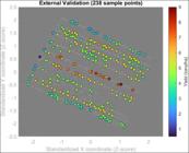
This evaluation enabled the comparison of spatial yield patterns and the impact of different resampling methods and validation sample sizes on model generalization. Subsequently, each GPR-fitted model was applied to a regular spatial grid covering the study area. This process allowed the interpolation of yield values at unsampled locations, which resulted in spatial yield maps. These interpolated yield maps facilitated the assessment of spatial yield patterns and the impact of different resampling methods and validation sample sizes on model performance, a critical challenge in spatial interpolation and predictive modeling.(¹⁴)

Additionally, a second experiment was conducted to compare the performance of GPR with OK and SVM, both implemented using the Smart-Map plugin in QGIS. In this case, the evaluations were also performed on the sample subsets presented in Figure 3, ensuring a consistent comparison across different dataset sizes.

The analysis relies on statistical metrics such as the coefficient of determination (R²), Root Mean Squared Error (RMSE) and Mean Absolute Error (MAE) to assess the prediction quality of each method under different sampling scenarios. While RMSE and R² evaluate accuracy (including relative RMSE – rRMSE), MAE was computed to quantify the average magnitude of the prediction errors, regardless of their sign. In contrast to RMSE, MAE is less sensitive to large deviations, whereas RMSE penalizes larger errors more strongly and therefore reflects both random variability and the presence of larger deviations in the estimates. When analyzed jointly with RMSE, MAE provides complementary information that may suggest the presence of non-random or persistent error patterns.

The RMSE measures the quadratic mean error between predicted and actual values and the relative RMSE (rRMSE %) expresses the RMSE as a percentage of the mean of the ground truth values, as follows:

(12) $RMSE =\sqrt{\frac{1}{n}\underset{i=1}{\overset{n}{\Sigma }}{\left(y_i-{ŷ}_1\right)}^2}$

(13) $rRMSE =\frac{RMSE}{\overline{y}}\times 100$

where y_i is the observed actual value of soybean yield, ŷ_i is the predicted value from GPR, y is the mean of the observed actual values, and n is the number of observations.

The MAE measures the absolute mean error between predicted and actual values:

(14) $MAE =\frac{1}{n}\underset{i=1}{\overset{n}{\Sigma }}\left|y_i-{ŷ}_i\right|$

The R² coefficient measures the proportion of variability in the data explained by the model:

(15) $R^2=1-\frac{\underset{i=1}{\overset{n}{\Sigma }}{\left(y_i-{ŷ}_i\right)}^2}{\underset{i=1}{\overset{n}{\Sigma }}{\left(y_i-\overline{y}\right)}^2}$

To assess generalization performance, k-fold cross-validation was conducted with k = 5, following the same procedure adopted in OK and SVM in Smart-Map QGIS.⁽¹³⁾

RESULTS AND DISCUSSION

Evaluation of GPR Performance Under Different Sample Sizes

The performance of GPR was evaluated across different sample sizes using internal (Int.) and external (Ext.) validation datasets. The evaluation of GPR across different sample sizes demonstrates a progressive decline in predictive accuracy as the sample size decreases (Table 2). The regression figures are provided in supplementary material.

Table 2
Statistical summary of sample sizes

Sample Size	RMSE (t/ha) (Int./Ext.)	MAE (t/ha) (Int./Ext.)	R2 (t/ha) (Int./Ext.)	rRMSE (%) (Int./Ext.)
Full Dataset (795 points)	0.47/-	0.33/-	0.86/-	9.64%/-
100% (557 points)	0.53/0.51	0.38/0.35	0.83/0.81	10.81%/10.66%
80% (446 points)	0.55/0.52	0.39/0.36	0.81/0.81	11.24%/10.76%
60% (334 points)	0.66/0.54	0.47/0.39	0.74/0.79	13.37%/11.17%
40% (223 points)	0.77/0.66	0.57/0.48	0.65/0.69	15.75%/13.70%
20% (112 points)	1.01/0.91	0.77/0.67	0.39/0.41	20.86%/18.91%

For the full dataset (795 sample points), the internal validation achieved an RMSE of 0.47, MAE of 0.33, and an R² of 0.86, with an rRMSE of 9.64%. The model performed well, capturing most of the variability in the data. When using 100% of the Int. dataset (557 points), the performance remained close to that of the full dataset, with an RMSE of 0.53 (Int.) and 0.51 (Ext.), MAE of 0.38 (Int.) and 0.35 (Ext.), and an R² of 0.83 (Int.) and 0.81 (Ext.). The relative RMSE (rRMSE) slightly increased to 10.81% for Int. and 10.66% for Ext., suggesting a minor decline in generalization capability.

As the sample size decreased to 80% (446 points), the performance degraded slightly, with RMSE increasing to 0.55 (Int.) and 0.52 (Ext.), MAE to 0.39 (Int.) and 0.36 (Ext.), while R² remained stable at 0.81 for both Int. and Ext. validation. The rRMSE increased slightly to 11.24% (Int.) and 10.76% (Ext.), indicating a marginal loss in predictive power.

At 60% (334 points), a more noticeable drop in performance occurred. The RMSE increased to 0.66 (Int.) and 0.54 (Ext.), and MAE increased to 0.47 (Int.) and 0.39 (Ext.), while R² declined slightly to 0.74 (Int.) and 0.79 (Ext.). The rRMSE increased to 13.37% (Int.) and 11.17% (Ext.), suggesting a greater loss in accuracy, particularly for internal validation. However, given that R² remained above 0.79, this sample size still provided a relatively robust model.

When reducing the dataset further to 40% (223 points), the performance deteriorated significantly. The RMSE increased to 0.77 (Int.) and 0.66 (Ext.), while MAE rose to 0.57 (Int.) and 0.48 (Ext.). The R² dropped more noticeably to 0.65 (Int.) and 0.69 (Ext.), reflecting a substantial reduction in model reliability. The rRMSE increased to 15.75% (Int.) and 13.70% (Ext.), showing a higher degree of error propagation.

With the smallest dataset, 20% (112 points), the model struggled considerably. The RMSE reached 1.01 (Int.) and 0.91 (Ext.), while MAE increased to 0.77 (Int.) and 0.67 (Ext.). The R² values plummeted to 0.39 (Int.) and 0.41 (Ext.), indicating a weak relationship between predictions and actual values. The rRMSE reached its highest values, at 20.86% (Int.) and 18.91% (Ext.), confirming that the model lacks robustness at this sample size.

The prediction maps generated for each sample size visually illustrate the impact of reducing the dataset (Figure 5). The full dataset (795 points) shows a well-defined structure of yield variability, with clear high- and low-yielding regions. As the sample size decreases, the prediction maps become progressively smoother, with less defined local spatial structures.

Figure 5
Soybean yield spatial prediction at different dataset sizes: (a) Full dataset (795 points), (b) 100% (557 points), (c) 80% (446 points), (d) 60% (334 points), (e) 40% (223 points), and (f) 20% (112 points).

From 100% (557 points) to 60% (334 points), the spatial patterns remain largely intact, demonstrating that GPR can still generalize well with moderate data reduction. However, at 40% (223 points), the prediction quality degrades significantly, as visible smoothing effects reduce the contrast in yield variability. The 20% (112 points) prediction map shows a severe loss of spatial resolution, with highly smoothed and less reliable predictions, further confirming the poor performance indicated by R² and RMSE.

The prediction maps further reinforce these findings, showing that the model maintains spatial coherence until 60%, after which the patterns degrade significantly. Thus, to ensure optimal GPR performance, a sample size of at least 60% should be maintained to balance predictive accuracy and dataset efficiency, while using 40% or less leads to significant performance degradation. These results suggest that, although accuracy metrics indicate a slight decline with lower sample densities, GPR retains its ability to capture yield spatial patterns. This is consistent with findings from,(¹⁰) who reported that GPR models provide excellent generalization ability even with small sample sizes.

The main limitation was not the GPR itself, but the insufficient number of samples, which prevented the model from effectively capturing local yield variations. The reduced sample density led to an oversmoothing effect, where finer spatial details were lost. These results highlight the importance of optimizing sample sizes to balance the trade-off between capturing detailed local patterns (which requires a higher number of samples) and reducing operational costs (which benefits from lower field sampling efforts). This balance is crucial in precision agriculture applications, where economic constraints often limit extensive data collection, yet spatial heterogeneity must be accurately represented for effective decision-making.

In general, while RMSE progressively increases with reduced sample size, R² remains stable up to 60%, meaning the model still captures most of the data variability. However, at 40%, a significant decline in R² (0.65 Int.) and an increase in RMSE (0.77 Int.) indicate the model starts losing predictive strength. At 20%, both R² and RMSE confirm that the model is no longer reliable, with R² dropping below 0.50 and RMSE surpassing 1.0, meaning prediction errors are large.

Performance Evaluation of GPR, Ordinary Kriging, and SVM in Yield Prediction

OK is the default interpolation method in the Smart-Map module. This method relies on the calculation of a semivariogram, which enables the analysis of the spatial dependence of soybean yield. To optimize performance, different semivariogram models were tested, and those with the lowest RMSE were selected. The analysis of the kriging interpolation parameters reveals that reducing the sample size directly influences estimation accuracy (Table 3). The best-fitting model was the exponential model, which was used for all cases. As the number of points decreases from 557 (100%) to 112 (20%), variations in both the R² and the RMSE indicate that the model's predictive performance is affected. However, contrary to a consistent decline in fit quality, the results suggest that adjusting spatial parameters can mitigate some of the negative effects of reduced data availability. Importantly, the maximum distance for interpolation was fixed at 60 m across all cases.

As the sample size decreases, the lag distance increases, ranging from 6.59 for the largest dataset to 13.58 for the smallest. This trend suggests that, with fewer available data points, the spacing between pairs used in the semivariogram becomes larger, potentially reducing the ability to capture finer spatial variations. Despite the reduction in sample size, the nugget effect (C0) remains zero across all cases, indicating that no unexplained small-scale variability or measurement noise is present.

The sill (C0 + C) remains relatively stable between 1.77 and 1.87, with the highest value observed for the 334-sample dataset. However, for the smallest sample size (112 points – 20%), the sill decreases to 1.65, suggesting a reduction in the total variance accounted for by the spatial model. Similarly, the range, which represents the spatial correlation distance, remains close to 57.5 m for most sample sizes but drops significantly to 46.92 m for the 112-sample dataset. This reduction suggests that with fewer data points, the detected spatial dependence is weaker.

The RMSE fluctuates across sample sizes, generally increasing as the dataset is reduced. However, an exception is observed for the 223-sample dataset, where RMSE decreases slightly compared to the 334-sample case. This suggests that, for certain sample sizes, the spatial model maintains good predictive performance despite a reduction in available data. The R² remains high for larger sample sizes but drops from 0.943 for 557 samples to 0.77 for 112 samples, indicating a loss of model reliability in the smallest dataset.

Overall, the results indicate that reducing the sample size influences kriging interpolation by affecting the range, sill, RMSE, and R². However, while a decrease in R² and an increase in RMSE are expected, the magnitude of these changes suggests that spatial parameters such as the lag and range should be carefully adjusted when working with limited data. The fact that C0 remains zero throughout the analysis suggests that the dataset is relatively clean, free of significant noise or measurement errors. The decrease in range for the smallest dataset highlights the importance of optimizing interpolation parameters to compensate for the loss of spatial correlation when working with fewer observations.

Table 3
Kriging interpolation parameters for each sample size

Sample Size	Lag (m)	C0	C0+C	Range(t/ha)	RMSE(t/ha)	R2
557 (100%)	6.59	0	1.80	57.84	0.09	0.94
446 (80%)	7.37	0	1.77	57.50	0.07	0.94
334 (60%)	7.37	0	1.87	57.49	0.14	0.92
223 (40%)	10.42	0	1.81	57.61	0.08	0.91
112 (20%)	13.58	0	1.65	46.92	0.14	0.77

For SVM, the choice of kernel function is a crucial hyperparameter. In the Smart-Map plugin, the Radial Basis Function (RBF) kernel is the default, as it has been found to be well-suited for most datasets due to its ability to capture nonlinear relationships.(¹¹)

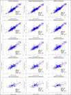
The spatial distribution of soybean yield is influenced not only by the choice of interpolation method but also by the sampling density used to generate yield maps. The results displayed in Figure 6 indicate that, although GPR, OK, and SVM achieved similar performance in cross-validation based on regression plots and statistical quality indicators (RMSE, MAE, R², and rRMSE), a smoothing effect was clearly present in the SVM-generated yield maps (Figure 7).

Figure 6
Regression Plots (Observed vs. Predicted Yield) for GPR, OK and SVM, respectively.

Figure 7
Yield spatial distribution using GPR, OK and SVM at different sample sizes.

The GPR model used in this study is anisotropic, employing a Rational Quadratic Kernel with a separate length scale per predictor. This structure allows GPR to model spatial relationships independently along each predictor axis, making it more flexible in capturing local variations than isotropic approaches such as OK, which rely on a single spatial dependency structure for all directions.

For larger sample sizes, GPR and OK exhibited similar performance, but GPR demonstrated a clear advantage when the number of sampled points was reduced (Figure 6). As the sample density decreased, the yield maps generated by SVM became increasingly smoothed, indicating that SVM struggled to capture fine-scale spatial variations, likely due to the limited number of support vectors available for training. This behavior suggests that SVM is less sensitive to local spatial trends, which can lead to an oversimplified representation of yield variation. In contrast, OK and GPR better preserved spatial patterns, with GPR showing superior adaptability in regions with fewer observations.

OK leverages the spatial dependence structure of the data via the semivariogram, making it well-suited for sparse datasets. However, the anisotropic GPR used in this study exhibited greater flexibility, as its kernel function allows it to learn distinct spatial scales for different predictor dimensions. This property becomes particularly relevant in fields with complex spatial structures, where different factors influence yield variability at different scales.

In scenarios with high spatial heterogeneity due to biotic and abiotic factors, GPR emerged as the most robust alternative. The observed yield variations in the study area were strongly influenced by soil properties, topography, and microclimatic differences. The heterogeneity of the Red Latosol, including variations in organic matter content, water retention capacity, and nutrient distribution, created complex spatial patterns that GPR captured with higher precision than OK and SVM. Additionally, topographical variations influenced soil moisture distribution and nutrient transport, further reinforcing the need for interpolation models that can account for such spatial complexity.

The spatial variability observed in soybean yield in the study area was driven by multiple interacting environmental, biological, and management-related factors. The field was located on a Red Latosol (Oxisol), a soil type characterized by high clay content, strong aggregation, and moderate natural fertility, where small-scale variations in organic matter, nutrient distribution, and water availability commonly generated heterogeneous crop responses. Gentle topographic undulations influenced runoff, infiltration, and soil moisture retention, creating localized zones of higher or lower productivity. Microclimatic conditions, including differences in solar radiation exposure, temperature gradients, and wind incidence further contributed to spatial variability, especially near the field borders where plants were exposed to greater environmental fluctuations. Border effects were particularly evident in this area, likely reflecting increased sensitivity to microclimate variability and edge-related stressors.

In addition to abiotic influences, biotic factors such as pest distribution and irregular crop emergence also played a role in shaping localized yield patterns. Historical management practices including tillage intensity, machinery traffic, crop rotation, and localized compaction may have left lasting spatial imprints on soil structure and nutrient availability. These combined factors explained the heterogeneous spatial distribution of soybean yield and clarified why interpolation methods differed in their ability to capture fine-scale variation. While GPR and OK were able to model these complex spatial patterns, SVM consistently produced over-smoothed predictions and failed to detect localized trends, particularly under reduced sample density. These observations reinforced that GPR exhibited the highest resilience to sampling reduction, followed by OK, whereas SVM showed the greatest loss of spatial detail under sparse data conditions. This underscores the importance of selecting interpolation methods that maintain stability and accuracy under different sampling scenarios. In precision agriculture, where accurate yield estimation is critical for optimizing input management and maximizing profitability, GPR stands out as a reliable option, particularly in environments with limited sample availability.

From a practical perspective, these findings confirm that anisotropic GPR is a powerful tool for yield mapping, providing a balanced trade-off between interpolation accuracy and computational efficiency. The ability of GPR to incorporate different spatial scales via its kernel function makes it a highly adaptable method for spatial prediction, ensuring robust and detailed yield estimates even in data-limited regions.

Despite these limitations, SVM has evolved into an efficient paradigm for handling nonlinear problems,(¹⁵) yet it struggles in spatial interpolation where spatial continuity is key. OK leverages the spatial dependence structure of yield data through the semivariogram, making it a suitable method in sparse data conditions. However, GPR’s structure, particularly with the Rational Quadratic Kernel with a separate length scale per predictor, ensures a higher level of detail in regions with fewer observations. GPR model fitting involves estimating covariance function parameters and noise variance, optimizing hyperparameters using maximum likelihood estimation (MLE). The model’s kernel function plays a fundamental role in adjusting to different spatial patterns, allowing GPR to capture finer spatial details more effectively than OK, especially when the sampling density is reduced.

For large sample sizes (e.g., 795 samples in this study area), GPR and OK performed similarly, both outperforming SVM. However, previous studies suggest that SVM may surpass OK in certain conditions, such as when dealing with high-dimensional feature spaces rather than pure spatial interpolation tasks.(¹³,¹⁶) On the other hand, research has also shown that GPR offers noticeable gains in terms of accuracy and robustness when compared to other machine learning approaches for soybean yield estimation.(⁵)

The differences observed between GPR, OK, and SVM in estimating soybean yield can be explained by various biotic and abiotic factors influencing spatial yield distribution in the field. Specifically, in this study area, soil variability and topography played crucial roles. The heterogeneity of soil properties, including organic matter content, water retention capacity, and nutrient availability in the Red Latosol, created complex spatial patterns that GPR captured more accurately due to its ability to model spatial autocorrelation through kernel functions and optimized hyperparameters. Topography also influenced the distribution of soil moisture and nutrients, which was better represented by GPR and OK.

Additionally, microclimatic variations within the study area, such as differences in solar radiation and temperature, likely contributed to spatial yield patterns. GPR and OK effectively modelled these variations, whereas SVM tended to produce overly smoothed predictions, failing to capture localized fluctuations. Among the biotic factors that impacted yield estimates, pest and disease distribution, uneven crop growth, and past agricultural management practices played key roles.(¹⁷) The irregular presence of soybean pests, such as caterpillars, created patches of low productivity, which GPR and OK identified more effectively due to their reliance on spatial dependence modelling. Uneven crop growth, resulting from emergence variability and intraspecific competition, also introduced complex patterns that GPR and OK captured with greater accuracy.

Furthermore, historical agricultural practices, such as variable-rate fertilization and crop rotation, left spatial imprints on yield distribution, which GPR and OK detected more effectively, whereas SVM may require a larger dataset to learn these spatial relationships.

The results suggest that GPR exhibited the least sensitivity to sample density reduction, followed by OK, while SVM suffered the most from data sparsity. This highlights the importance of selecting interpolation models that maintain stability under different sampling conditions, reinforcing that GPR is the most resilient option in this study. In soybean cultivation, characterized by its specific nutritional requirements and strong dependence on climatic conditions, the ability to accurately detect yield variations can mean the difference between a profitable harvest and significant losses.(¹⁸)

From a practical standpoint, these findings confirm that GPR is a valuable tool for precision agriculture applications, particularly when sample availability is limited. The balance between interpolation accuracy and computational efficiency makes GPR a promising alternative for large-scale yield mapping. Furthermore, its kernel-based structure allows for flexible adaptation to different spatial patterns, ensuring robust predictions even in regions with fewer observations.

CONCLUSIONS

This study evaluates the impact of interpolation methods and sample size reduction on soybean yield prediction. GPR and OK consistently outperform SVM, with GPR showing the highest robustness to sample size reduction. OK remains effective but is more sensitive to sample density and relies on the assumption of isotropy, which may not always hold in agricultural fields. SVM in Smart-Map suffers the most from data sparsity, producing smoother estimates and failing to capture finer spatial variations. However, optimizing SVM with a more suitable kernel function could enhance its performance. From a practical perspective, GPR and OK remain strong candidates for yield interpolation, reinforcing the importance of selecting methods based on data availability and spatial variability to ensure accurate predictions in precision agriculture.

A preprint version is published and available from: https://doi.org/10.1590/SciELOPreprints.11312(¹⁹)

ACKNOWLEDGMENTS, FINANCIAL SUPPORT AND FULL DISCLOSE

The authors acknowledge the institutional support and resources provided for the development of this study. This work was funded by the Brazilian Federal Agency for Support and Evaluation of Graduate Education (CAPES) through a scholarship awarded to Samuel Philippe. Additionally, this study received financial support from the National Council for Scientific and Technological Development (CNPq), process no. 421278/2023-4, linked to the first author. This work was also supported by CNPq (grant no. 309248/2025-6) awarded to the first author.

The authors declare that there are no conflicts of interest

• 1
  Excerpt from the dissertation work by Samuel Philippe submitted to the Programa de Pós-Graduação em Agricultura e Informações Geoespaciais (PPGAIG).

DATA AVAILABILITY STATEMENT

Data can be provided upon request to the authors by contacting the corresponding author via email.

REFERENCES

• ¹ Lucas MP, Longman RJ, Giambelluca TW, Frazier AG, McLean J, Cleveland SB, et al. Optimizing automated kriging to improve spatial interpolation of monthly rainfall over complex terrain. J Hydrometeorol. 2022;23(4):561-72. doi:10.1175/JHM-D-21-0171.1.
  » https://doi.org/10.1175/JHM-D-21-0171.1
• ² Sifaou H, Kammoun A, Alouini MS. A precise performance analysis of support vector regression. In: Proceedings of the 38th International Conference on Machine Learning (ICML); 2021. p. 9671-80.
• ³ Siqueira DS, Barros JGA, Marques JS, Pereira GT. Geostatistical and machine learning models for spatial prediction of soil properties in precision agriculture. Revista Ceres. 2021;68(5):384-93. doi:10.1590/0034-737X202168050008.
  » https://doi.org/10.1590/0034-737X202168050008
• ⁴ Campos-Taberner M, García-Haro FJ, Moreno Á, Gilabert MA, Sánchez-Ruiz S, Martínez B, et al. Mapping leaf area index with a smartphone and Gaussian processes. IEEE Geosci Remote Sens Lett. 2015;12(12):2501-5. doi:10.1109/LGRS.2015.2488682.
  » https://doi.org/10.1109/LGRS.2015.2488682
• ⁵ Martínez-Ferrer L, Piles M, Camps-Valls G. Crop yield estimation and interpretability with Gaussian processes. IEEE Geosci Remote Sens Lett. 2021;18(12):2043-7. doi:10.1109/LGRS.2020.3016140.
  » https://doi.org/10.1109/LGRS.2020.3016140
• ⁶ Alebele Y, Wang W, Yu W, Zhang X, Yao X, Tian Y, et al. Estimation of crop yield from combined optical and SAR imagery using Gaussian kernel regression. IEEE J Sel Top Appl Earth Obs Remote Sens. 2021;14:10520-34. doi:10.1109/JSTARS.2021.3118707.
  » https://doi.org/10.1109/JSTARS.2021.3118707
• ⁷ Martins GD, Xavier LCM, Oliveira GP, Gallo MLBT, Abreu Júnior CAM, Vieira BS, et al. Using geospatial information to map yield gain from the use of Azospirillum brasilense in furrow. Agronomy. 2023;13(3):808. doi:10.3390/agronomy13030808.
  » https://doi.org/10.3390/agronomy13030808
• ⁸ Alvares CA, Stape JL, Sentelhas PC, Gonçalves JLM, Sparovek G. Köppen’s climate classification map for Brazil. Meteorol Z. 2013;22(6):711-28. doi:10.1127/0941-2948/2013/0507.
  » https://doi.org/10.1127/0941-2948/2013/0507
• ⁹ Climate-Data.org. Climate of Patos de Minas. 2024 [cited 2025 Sep 8]. Available from: https://en.climate-data.org/south-america/brazil/minas-gerais/patos-de-minas-2893/
  » https://en.climate-data.org/south-america/brazil/minas-gerais/patos-de-minas-2893/
• ¹⁰ He H, Zheng T, Zhao J, Yuan X, Sun E, Li H, et al. Improved Gaussian regression model for retrieving ground methane levels by considering vertical profile features. Front Earth Sci. 2024;12:1352498. doi:10.3389/feart.2024.1352498.
  » https://doi.org/10.3389/feart.2024.1352498
• ¹¹ Rasmussen CE, Williams CKI. Gaussian processes for machine learning. Cambridge (MA): MIT Press; 2006. 266p.
• ¹² Rodrigues BP, Rofatto VF, Matsuoka MT, Assunção TT. Resampling in neural networks with application to spatial analysis. Geospat Inf Sci. 2022;25(3):413-24. doi:10.1080/10095020.2022.2040923.
  » https://doi.org/10.1080/10095020.2022.2040923
• ¹³ Pereira GW, Valente DSM, Queiroz DMD, Coelho ALDF, Costa MM, Grift T. Smart-map: an open-source QGIS plugin for digital mapping using machine learning techniques and ordinary kriging. Agronomy. 2022;12(6):1350. doi:10.3390/agronomy12061350.
  » https://doi.org/10.3390/agronomy12061350
• ¹⁴ Li J. A critical review of spatial predictive modeling process in environmental sciences with reproducible examples in R. Appl Sci. 2019;9(10):2048. doi:10.3390/app9102048.
  » https://doi.org/10.3390/app9102048
• ¹⁵ Chandra MA, Bedi SS. Survey on SVM and their application in image classification. Int J Inf Technol. 2021;13(5):1-11. doi:10.1007/s41870-017-0080-1.
  » https://doi.org/10.1007/s41870-017-0080-1
• ¹⁶ Ribeiro JL, Silva AM. Comparative study of kriging and support vector machines for spatial prediction of soil properties. Comput Electron Agric. 2018;155:183-93.
• ¹⁷ Carvalho E, Assis GA, Martins GD, Marques DJ, Santos EA, Xavier LCM, et al. Intercropped soybean plant population in a coffee plantation and its effects on agronomic parameters and geospatial information. Agronomy. 2024;14(2):343. doi:10.3390/agronomy14020343.
  » https://doi.org/10.3390/agronomy14020343
• ¹⁸ Filippi P, Han SY, Bishop TF. On crop yield modelling, predicting, forecasting and addressing the common issues in published studies. Precis Agric. 2025;26(1):8. doi:10.1007/s11119-024-10212-2.
  » https://doi.org/10.1007/s11119-024-10212-2
• ¹⁹ Rofatto VF, Philippe S, Martins GD. Gaussian process regression as an alternative to kriging and SVM for spatial yield prediction. SciELO Preprints. 2025. doi:10.1590/SciELOPreprints.11312.
  » https://doi.org/10.1590/SciELOPreprints.11312

Edited by

• Editors:
  Maicon Nardino
  Marihus Baldotto

Publication Dates

• Publication in this collection
  16 Mar 2026
• Date of issue
  2026

History

• Received
  08 Oct 2025
• Accepted
  21 Jan 2026

• This document has a preprint version
  10.1590/SciELOPreprints.11312