Accounting for spatial runoff variability in LID design for urban catchments: model and software development

Consideração da variabilidade espacial do escoamento superficial no projeto de LID para bacias urbanas: desenvolvimento de modelo e software

ABSTRACT

This study presents an integrated approach for the design of lot-scale micro-reservoirs that considers the spatial variability of runoff generation within a catchment. Traditional reservoir sizing methods often neglect the cumulative, catchment-scale hydrological effects, which can lead to unintended synchronization of hydrograph peaks and localized flooding. The proposed methodology introduces a novel design criterion based on the upstream hydrological contribution and the position of each lot within the catchment. Using the Rational Method for runoff estimation, the SCS–CN method for infiltration and abstraction losses, and the PULS method for hydraulic routing, an open-source Excel–VBA tool was developed to automate the modeling and design process. Three case studies demonstrate the framework's ability to distinguish design requirements for lots with identical geometries but varying catchment positions. Results show that reference flow constraints derived from upstream characteristics significantly influence the required storage volume and outlet configuration. The tool supports optimization and performance analysis through dimensionless indicators that characterize peak attenuation, time-to-peak delay, storage performance, and mass balance.

Keywords:
Lot-scale reservoir design; Urban stormwater management; Catchment-scale hydrology; Low-Impact Development (LID); Hydrologic-hydraulic modeling

RESUMO

Este estudo apresenta uma abordagem integrada para o dimensionamento de microreservatórios em escala de lote, considerando a variabilidade espacial da geração de escoamento dentro de uma bacia hidrográfica. Métodos tradicionais de dimensionamento frequentemente negligenciam os efeitos hidrológicos cumulativos em escala de bacia, o que pode levar à sincronização indesejada de picos de vazão e à ocorrência de alagamentos localizados. A metodologia proposta introduz um novo critério de projeto baseado na contribuição hidrológica a montante e na posição de cada lote dentro da bacia. Utilizando o Método Racional para estimativa de escoamento, o método SCS-CN para perdas por infiltração, e o método PULS para a propagação hidráulica, foi desenvolvida uma ferramenta computacional de código aberto em Excel-VBA para automatizar o processo de modelagem e dimensionamento. Três estudos de caso demonstram a capacidade do modelo em distinguir requisitos de projeto para lotes com geometria idêntica, mas com diferentes posições na bacia. Os resultados mostram que restrições de vazão de referência derivadas das características a montante influenciam significativamente o volume de armazenamento necessário e a configuração dos dispositivos de saída. A ferramenta permite análise de sensibilidade e otimização por meio de indicadores adimensionais, promovendo a resiliência dos sistemas de drenagem urbana. Este framework viabiliza o dimensionamento sensível ao contexto, conectando a implementação local ao controle de cheias em escala de bacia.

Palavras-chave:
Dimensionamento de reservatórios em escala de lote; Gestão de drenagem urbana; Hidrologia em escala de bacia; Desenvolvimento de Baixo Impacto (DBI); Modelagem hidrológica-hidráulica

INTRODUCTION

The design of urban drainage systems is significantly influenced by changes in land use and land cover, altering pre-development hydrology to post-development hydrologic conditions with flashier and more intense flow peaks; this effect is often referred to as the “urban stream syndrome” (Vietz et al., 2016; Walsh et al., 2005). In residential developments such as condominiums, sewer and drainage subsystems, once designed assuming a land use and land cover imperviousness rate, can be impacted by increased urbanization that was not considered at the lot scale (Bibi et al., 2023). This effect generates more runoff and shifts the pre-development hydrological behavior of the sub-catchment to a post-urbanization regime. Although interesting from the hydrological standpoint, the requirement for larger green areas in construction codes presents a limitation for the use of effectively constructed areas in a residential lot. Alternatively, effectively designed gray and green infrastructure, with higher drainage and storage capacity, can compensate for the increase in impervious areas (Fileni et al., 2019; Costa et al., 2020).

Low-impact development techniques, such as lot-scale reservoirs, can mitigate increasing runoff (Dornelles et al., 2010; Tassi & Villanueva, 2004). They function as decentralized detention ponds, equipped with controlled outflow devices such as orifices conveying regular flows and emergency spillways conveying excess runoff. This ensures regulated, delayed, and controlled outflows if adequately designed. However, the decentralized nature of source control techniques shifts operation and maintenance responsibilities to individual property owners (Baptista et al., 2017). Without an integrated management strategy at the catchment scale, inconsistent maintenance practices may compromise the system's overall efficiency. Nonetheless, maintenance requirements are relatively straightforward, primarily involving complete evacuation of stored water, inspection of hydraulic devices, and cleaning at least once per year (Baptista et al., 2017). In residential condominium areas, an effective, regular management process can be implemented to ensure the proper maintenance of these LID structures. The implementation of lot-scale micro-reservoirs depends on topographic conditions, as they must be directly connected to the receiving drainage infrastructure by gravity whenever possible. Retrofitting these systems in already developed areas can be challenging, especially if main drainage lines have been installed. However, low-impact development (LID) strategies can be integrated into the initial planning phase in new condominium developments. By incorporating designated lot connections within the drainage network layout, developments can accommodate future increases in imperviousness while minimizing the need for costly upgrades to the primary drainage system.

Regulatory frameworks for lot-scale micro-reservoirs have been introduced in Brazil over the past few decades. Yet, the design criteria remain inconsistent, often being either overly simplified or excessively complex (Prefeitura de Belo Horizonte, 2022; Tucci, 1997; São Paulo, 2007). Some methodologies rely on assumptions that are difficult to validate in practice, leading to inaccuracies in volume estimation. For instance, the method proposed by McCuen (1998) considers pre- and post-urbanization conditions but does not account for the outflow hydrograph characteristics, such as peak discharge timing and shape. Consequently, a reservoir designed solely to meet volumetric requirements may still fail to mitigate peak flow and peak time if the outlet configuration is inadequate (Gomes Junior et al., 2023). For example, an oversized outlet structure may allow the reservoir to discharge too quickly, returning hydrographs to the receiving drainage system with little or no attenuation effect (Gomes Junior et al., 2024).

Typically, the design of lot-scale reservoirs is made solely based on the upstream catchment of the lot's contribution to the runoff (i.e., roofs, parking lots, and backyards). By employing a sub-catchment hydrological routing method and, later, a reservoir hydraulic routing, one can estimate the hydraulic behavior of a lot-scale reservoir for a given rainfall event relatively straightforwardly. From the viewpoint of the individual lot, the reservoir can appear to reduce peaks and volumes. From the catchment-scale standpoint, however, the reservoir outlet peak can be matched with the catchment peak discharge, hence providing limited effective reduction at the catchment scale. The identified challenge is, therefore, to design “locally” but analyze the performance “globally” (Baptista et al., 2017).

Another approach is presented in Tucci (2002). This method was applied in the drainage regulations of Porto Alegre, Brazil, and defines a minimum volume based on catchment imperviousness, the critical duration of the design storm, the admissible risk, and a specific restriction discharge, which can be interpreted as the pre-development discharge. The volume is analytically obtained; however, the system response outlet hydrograph is not considered for either outlet dimension, which may result in poorly designed lot-scale reservoirs.

Another example is observed in Silveira & Goldenfum (2007). The Curva-Envelope method explicitly analyzes the necessary reservoir volume, assuming that the reservoir should release a constant pre-development flow during the whole design event, and focuses on maximizing the accumulated difference between precipitated depth and outflow pre-development depth. Due to the non-linear behavior of the stage–discharge relationship, assuming a constant outflow under an unsteady inflow hydrograph is hydraulically inconsistent.

Approaches like those in numerical software, such as the Stormwater Management Model (SWMM) (Rossman, 2010) or the Hydrologic Engineering Center – Hydrologic Modeling System (HEC-HMS), allow users to perform hydrologic and hydraulic routing simulations and estimate the system outlet hydrograph. However, these are not dedicated design tools and require greater user expertise to optimize lot-scale reservoir designs; a standardized solution for the analysis and design of lot-scale reservoirs would therefore be helpful. The literature is clear that attempts to approach the problem in a simplified way, sometimes even analytically, are aimed at its use in drainage plans and its wide application. Nevertheless, most criteria used in these methods consider only local aspects at the lot scale, such as land-use occupation within the lot. The uneven generation of runoff throughout the catchment makes the use of constant specific pre-development discharges hydrologically incorrect, as it neglects the non-linear flood-wave travel and the variations in runoff generation with upstream topography. This study proposes an integrated approach, simplified enough to be implemented in spreadsheets, to design lot-scale reservoirs while explicitly accounting for both lot-scale and catchment-scale characteristics. Although the methods are presented for lot-scale micro-reservoirs, the approach can be readily adapted to other types of LID infrastructure by modifying the flood-routing functions to represent alternative LID configurations. This paper is structured as follows: Section 2 presents the model and the tool-guided interfaces used to run it; Section 3 introduces three numerical examples; Section 4 presents the results; Section 5 provides a discussion; and Section 6 summarizes the main conclusions.

MATERIALS AND METHODS

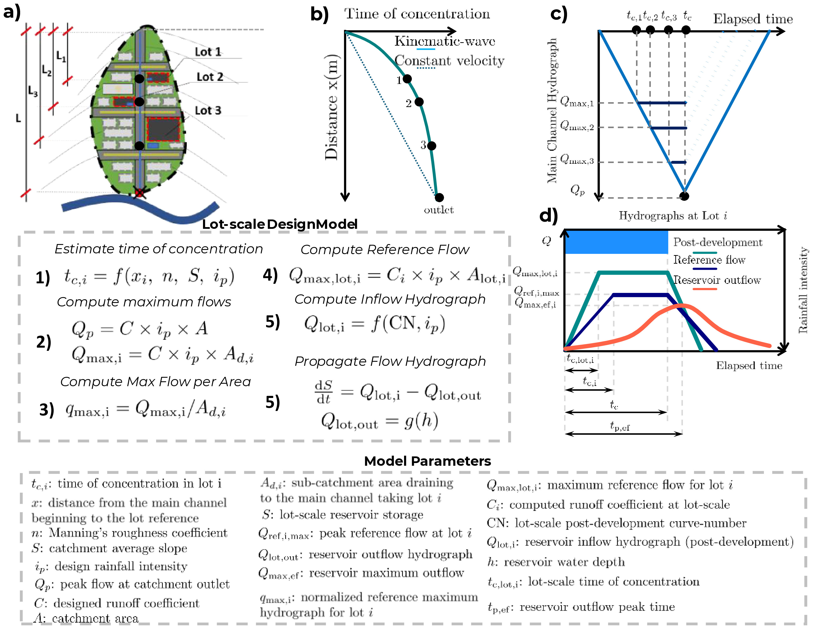
The model herein proposed is a catchment-based framework for designing lot-scale reservoirs that links local hydrological behavior to catchment-scale constraints. It assumes that lots with the same size and imperviousness may require different storage and outlet configurations depending on their upstream contributing area and their location along the drainage network. The procedure follows four steps: (i) derive reference constraints at the lot scale using the Rational Method and time of concentration to define the maximum admissible outflow and minimum allowable peak timing; (ii) estimate lot-scale runoff generation from effective rainfall using the SCS-CN method and an event-specific runoff coefficient; (iii) construct the lot inflow hydrograph with the Rational Method based on the lot’s time of concentration; and (iv) apply hydraulic routing with the PULS method to obtain the outflow hydrograph from the reservoir. The design is accepted if the simulated outflow does not exceed the reference discharge and if the peak occurs no earlier than the defined threshold. A schematic of the problem to estimate the reference hydrographs is shown in Figure 1.

Figure 1
Problem schematics, where (a) shows a plan representation of a small, urbanized catchment with a main urban drainage channel. Distances L are taken from the main channel reference. Grey dashed boxes represent residential areas, whereas black, red dashed boxes represent lots that will be designed in the examples presented in this manuscript. The blue box represents a small rectangular detention pond, and the red crossed circle is the catchment outlet. In (b), a schematic of the non-linear kinematic-wave time of concentration is shown, indicating this variable for lots 1, 2, 3, and for the outlet. For reference, a constant-velocity scheme is contrasted with deviations from a simpler time-of-concentration method toward a physically based approach. Part (c) shows the hydrograph at section x₁, x₂, x₃ (representing the lots' position), and at the outlet. If normalized by their upstream sub-catchment area, these hydrographs can represent the maximum flow discharge per area that a lot can convey to the receptor drainage system. The dark blue lines indicate a constant-flow hydrograph due to rainfall duration exceeding the reference time of concentration, and the dotted cyan lines are the recession hydrographs at these sections. The brief summary of the pseudocode for the simulation is shown in steps (1) to (5) with model parameters below, later fully described in the paper, and part (d) shows a schematic representation of the flow propagation in a lot-scale reservoir designed with the methods presented in this paper.

Mathematical model description

The catchment-scale hydrograph located at the lot-scale reservoir outlet system (i.e., typically a manhole at the street or a connecting point at the underlying sewer drain) can be modeled by the Rational Method. Most typically, urban drainage designs assume the rational method as the rainfall-runoff model, and here, I hypothesize that the main drainage pipeline at a small catchment is designed with this method. Equations (1)-(3) indicate the peak discharge at the catchment outlet, the peak discharge considering the lot-scale reservoir outlet, and the normalized hydrograph at the lot reference, such that:

$Q_{\text{max}}=C\times i_{\text{p}}\times A/3600$ (1)

$Q_{\text{max},\text{i}}=\left(\frac{t_{\text{c},\text{i}}}{t_{\text{c}}}\right)\times Q_{\text{max}}$ (2)

$q_{\text{max},\text{i}}=\frac{\left(\frac{t_{\text{c},\text{i}}}{t_{\text{c}}}\right)\times Q_{\text{max}}}{{\text{A}}_{\text{d},\text{i}}}=\frac{Q_{\text{max},\text{i}}}{A_{\text{d},\text{i}}},$ (3)

where Q_max is the maximum flow at the catchment outlet [L T^-3]. Q_max,i is the maximum flow of the receptor system at the lot i [L T^-3]. q_i is the specific flow of the system’s upstream sub catchment of lot i [L T^-1], A is the catchment area [L²], A_d,i is the sub-catchment of lot i system’s drainage area [L²], i_p is the precipitation rate given by a Sherman equation with the duration equals the catchment time of concentration [L T^-1]. From now on, catchment refers to the region defined by the drainage to the outlet, whereas sub-catchments are the regions draining to the lot-scale reference x_i taken from the main channel beginning, and the lot contributing area is the lot’s area draining to the lot-scale reservoir.

The time of concentration can be calculated by the Kinematic Wave in a plan, adaptable to catchments smaller than 0.5 km² (i.e., typically the case of small, urbanized catchments), according to Akan (1993), given by:

$t_{\text{c},\text{i}}\left(\text{x}\right)=447\times \left[\frac{{\left(x_i\times n\right)}^{0.60}}{{\left(\frac{K\times {\text{RP}}^{\text{a}}}{{\left(b+t_{\text{c},\text{i}}\right)}^{\text{c}}}\right)}^{0.4}\times {\text{S}}^{0.3}}\right],$ (4)

where t_c,i is the sub-catchment time of concentration taken the lot i as the reference outlet [s], index i represents the i^th lot in the catchment, x_i is the lot’s linear position in meters considering the farthest hydraulic point alongside the main sewer underdrain [m], n is the catchment weighted average Manning-Stricker coefficient for the sub-catchment [s m^-1/3], S is the average slope in m/km, RP is the return period [years], and K, a, b and c are the Sherman IDF parameters (Gomes Junior et al., 2019). The problem is iterative and usually converges with 3 or 4 attempts. As a first attempt, it is possible to use Kirpich’s equation (Silveira, 2005).

$t_{\text{c},\text{i}}=57\times {\left(\frac{x_{\text{i}}{}^2}{S}\right)}^{0.385}.$ (5)

From Equation (3), the factor (t_c,i / A_d,i) captures the hydrological response of the upstream reference catchment that governs the maximum reference flow (i.e., the maximum flow that the lot can convey without exceeding the design discharge at the receiving drainage system). This factor depends on land use (i.e., terrain roughness), the topography of the upstream catchment, and the catchment hypsometry that defines the upstream area. Larger areas with shorter times of concentration (e.g., catchments with a higher circularity index) produce larger reference outflows and thus contribute more to peak runoff at the catchment outlet. In these cases, the reference outflow for a lot located in such areas is larger, and the reservoir could be designed to release larger outflows. The first constraint in the lot-scale reservoir design is hence the maximum outlet flow. A well-designed lot-scale reservoir should respect a maximum reference outflow and a minimum peak time given by the restrictions of the catchment-scale hydrograph. The maximum reference outflow for the i^th reservoir in the catchment is given by:

$Q_{\text{ref},\text{i}}\left(\text{t}\right)=q_{\text{i}}\times A_{\text{lot},\text{i}},$ (6)

where Q_ref,i(t) is the reference outflow hydrograph [L T^-3] which the lot is restricted by, q_i is the normalized hydrograph per sub-catchment area of lot i [L T^-1], and A_lot,i is the lot’s drainage area [L²] with its maximum value defined by Q_ref,i,max.

Once the catchment-scale restrictions are defined, the lot-scale hydrological response must be estimated at the lot area. By employing a rainfall-runoff approach, the lot scale reservoir inflow hydrograph can be determined by the SCS-CN method combined with the Rational Method (Mulvaney, 1850; Kuichling, 1889). The latter assumes no temporal or spatial variation in rainfall, which is a fair assumption for small urban catchments (Canholi, 2015). Instead of assuming constant runoff coefficients based on land use and land cover, runoff coefficients are estimated based on soil infiltration capacity. The individual lot-scale contributing area infiltration potential is given by SCS-CN method (Mishra & Singh, 2013):

$S_{\text{i}}^c=\frac{25400}{{\text{CN}}_{\text{i}}}-\mathrm{254,}$ (7)

where S^c_i is the soil infiltration potential in mm, and CN_i is the lot-scale average curve number. The initial abstraction (I_a) can be estimated as a function of the infiltration potential, and can be obtained by:

$\mathrm{0,1}\times {\text{S}}_{\text{i}}^{\text{c}}\le {\text{I}}_{\text{a}}\le 0.2\times {\text{S}}_{\text{i}}^{\text{c}},$ (8)

where I_a are the initial losses [mm] and can be calibrated or adopted for the catchment.

The effective precipitation that generates overland flow runoff can be estimated by the SCS-CN method:

$P_{\text{ef},\text{i}}\left(\text{t}\right)=\frac{{\left(P_{\text{i}}\left(\text{t}\right)-I_{\text{a}}\right)}^2}{\left(P_{\text{i}}\left(\text{t}\right)+0.8\times S_{\text{i}}^{\text{c}}\right)}$, If $P_{\text{i}}\left(\text{t}\right)\ge I_{\text{a}}$, Else $P_{\text{ef},\text{i}}\left(\text{t}\right)=\mathrm{0,}$(9)

where P_ef,i(t) is the effective cumulated rain depth in time t [mm], P_i(t) is the total rain depth in time t [mm]. If one assumes the maximum rainfall duration as the catchment time of concentration t_c, the event effective precipitation P_ef,i at the lot-scale can be estimated using Equation (9).

Finally, the event-varying runoff coefficient can be written as:

$C_{\text{i}}=\frac{P_{\text{ef},\text{i}}}{P},$ (10)

where C_i is the runoff coefficient using the lot-scale time of concentration as rainfall duration [-] and P is the total event volume [L] with rainfall intensity i_p [L T^-1] and duration t_c [T].

The advantages of estimating the runoff coefficient rather than assuming a constant value stem from reduced model parametrization and from the ability to adopt an event-varying approach based on time-varying infiltration estimates using the SCS-CN infiltration method.

Once the lot-scale runoff coefficient is defined, one can estimate the synthetic inflow hydrograph at the lot-scale reservoir using the Rational Method as the conceptual model to convert excess precipitation into runoff. Other types of rainfall temporal distributions and conceptual rainfall-runoff models can be tested, but are out of the scope of this manuscript. In this case, however, the same rainfall–runoff approach used in the design of the drainage system is adopted, rather than applying the unit-hydrograph theory, to maintain consistency. In addition, by the rational method assumptions, the maximum inflow occurs at the lot scale time of concentration (t_c,lot,i) and, afterward, remains constant until the time of concentration of the catchment outlet since the rainfall ceases only after catchment t_c. The maximum inflow in the reservoir Q_max,lot,i is obtained by the rational method in Equation (11), given in L/s by:

$Q_{\text{max},\text{lot},\text{i}}=C_{\text{i}}\times i\times A_{\text{lot},\text{i}}/3600$ . (11)

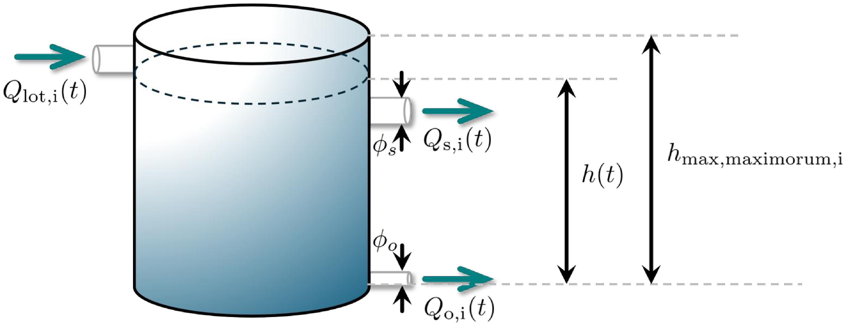
By estimating the peak flow Q_max,lot,i and the lot time of concentration t_c,lot,i, one can develop a rational method for the inflow hydrograph Qlot,i(t) as the inflow boundary condition for the lot-scale reservoir. To calculate the lot-scale reservoir outflow, a hydraulic routing is performed using the PULS method (Baptista et al., 2017; Canholi, 2015). Figure 2 is a schematic lot-scale reservoir showing, for a time t, the water balance.

Figure 2
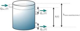
Lot-scale reservoir and its hydraulic devices for a double outlet where ϕ_s, ϕ_h, are the diameter of the orifice and spillway, respectively, and h(t) is the water depth. The maximorum height (h_{max,maximorum}) defines the maximum water depth h. The orifice is assumed to be without any internal water storage below, and the spillway centerline is defined at the elevation c_s from the reservoir bottom.

The PULS method considers a pool level horizontal water surface, neglecting hence advective, inertial, and diffusive effects at the reservoir surface, with only mass and energy conservation as the main governing equations to be solved (Ferreira et al., 2019; Gomes Junior et al., 2023). The water balance equations are given by Equations (12) and (13).

$\frac{\text{d}S}{\text{d}t}=Q_{\text{lot},\text{i}}\left(\text{t}\right)-Q_{\text{out},\text{i}}\left(\text{t}\right)$ (12)

$Q_{\text{out},\text{i}}\left(\text{t}\right)=Q_{\text{s},\text{i}}\left(\text{t}\right)+Q_{\text{h},\text{i}}\left(\text{t}\right)=f\left(\text{h}\right),$ (13)

where dS/dt is the storage variation in the reservoir [L T^-1], t is the time [T], Q_out,i(t) is the reservoir outflow in time t [L T^-3], and h is the water depth in the reservoir [L]. The function $f\left(h\right)$ models the reservoir stage-discharge relationship.

Integrating Equation (12) using an explicit finite-difference scheme for the time derivative and a centered-in-time approximation over a time step Δt, one obtains Equation (14):

$\begin{array}{c}{\text{Q}}_{\text{lot},\text{i}}\left(\text{t}\right)+{\text{Q}}_{\text{lot},\text{i}}\left(t+\Delta \text{t}\right)+\\ \left(\frac{2S\left(t\right)}{\Delta \text{t}}-{\text{Q}}_{\text{out},\text{i}}\left(\text{t}\right)\right)=\left(\frac{2S\left(t\right)}{\Delta \text{t}}+{\text{Q}}_{\text{out}}\left(\text{t}\right)\right).\end{array}$ (14)

The right-hand side terms of Equation (14) are known for t = t₀, where t₀ is the beginning of the simulation. By tabulating the term (2S/Δt + Q_out) for finite values of water depth h, one can estimate the left terms of Equation (14) and later obtain the outflow for the next time-step by isolating Q_lot,i(t + Δt) in this equation. This can be easily done with lookup functions. To this end, it is necessary to establish a relationship between the outflow and a storage factor. This relationship can be obtained by using standard hydraulic equations and least-squares fits of the reservoir stage-storage data. The stage-storage relationship can be fit in a geometrical curve given by Equation (15), such that:

$S=b\times h^c,$ (15)

where b has dimension [m]^(3-c), and c is a dimensionless constant, with h given in [m]. If c = 1, b is the prismatic surface area.

In practice, the reservoir is often discretized into a table relating water level to storage volume, which is typical for small detention ponds. Considering this table, a least square fit can be used to determine the stage-storage relationship to obtain b and c parameters in the Equations (16) and (17), such that:

$c=\frac{\left({{\displaystyle \sum }}_{\text{k}=1}^{\text{N}}\ln h_{\text{k}}\right)\times \left({{\displaystyle \sum }}_{\text{k}=1}^{\text{N}}\ln S_{\text{k}}\right)-N\times {{\displaystyle \sum }}_{\text{k}=1}^{\text{N}}(\ln h_{\text{k}}\times \ln S_{\text{k}})}{{\left({{\displaystyle \sum }}_{\text{k}=1}^{\text{N}}\ln h_{\text{k}}\right)}^2-\text{N}\times {{\displaystyle \sum }}_{\text{k}=1}^{\text{N}}{\left(\ln h_{\text{k}}\right)}^2}$ (16)

$b={\text{e}}^{\frac{{{\displaystyle \sum }}_{\text{k}=1}^{\text{N}}\left(\ln h_{\text{k}}\times \ln S_{\text{k}}\right)-c\times {{\displaystyle \sum }}_{\text{k}=1}^{\text{N}}{(\ln h_{\text{k}})}^2}{{{\displaystyle \sum }}_{\text{k}=1}^{\text{N}}\ln h_{\text{k}}}}$ (17)

where h_k and S_k is the water level and the storage in level k and N is the stage-storage vector size.

Once a continuous stage-storage relationship is defined, Equation (15) can be differentiated with respect to h to obtain the stage-area-volume relationships. To obtain a solution to Equation (14), all outlet-stage discharge devices must be modeled. The function that describes the outflow can be defined using standard hydraulic formulae by substituting Equation (18) into Equation (13), resulting in:

$Q_{\text{out},\text{i}}\left(\text{t}\right)=C_{\text{d},\text{o}}\times A_{\text{o}}\times \sqrt{2g{h}_{\text{o}}}+C_{\text{d},\text{s}}\times A_{\text{s}}\times \sqrt{2g{h}_{\text{s}}}$ (18)

$h_{\text{o}}=\max \left(h\left(t\right)-\frac{{\varphi }_h}{2}\mathrm{,0}\right)$ (19)

$h_{\text{s}}=\max \left(h\left(\text{t}\right)-(c_{\text{s}}+\frac{{\varphi }_{\text{s}}}{2})\mathrm{,0}\right),$ (20)

where C_d,o is the orifice discharge coefficient [-], C_d,s is the spillway discharge coefficient [-], and c_s is the spillway elevation [L]; flow discharge equations assume an atmospheric outlet boundary condition, although other conditions can be easily implemented in the model.

The discharge coefficient varies with the orifice diameter and its hydraulic head. An estimate for it can be found in Porto (2006) (see Supplementary Material). Correcting the discharge coefficient based on the outlet shape and position can enhance simulation accuracy, as the developed model considers.

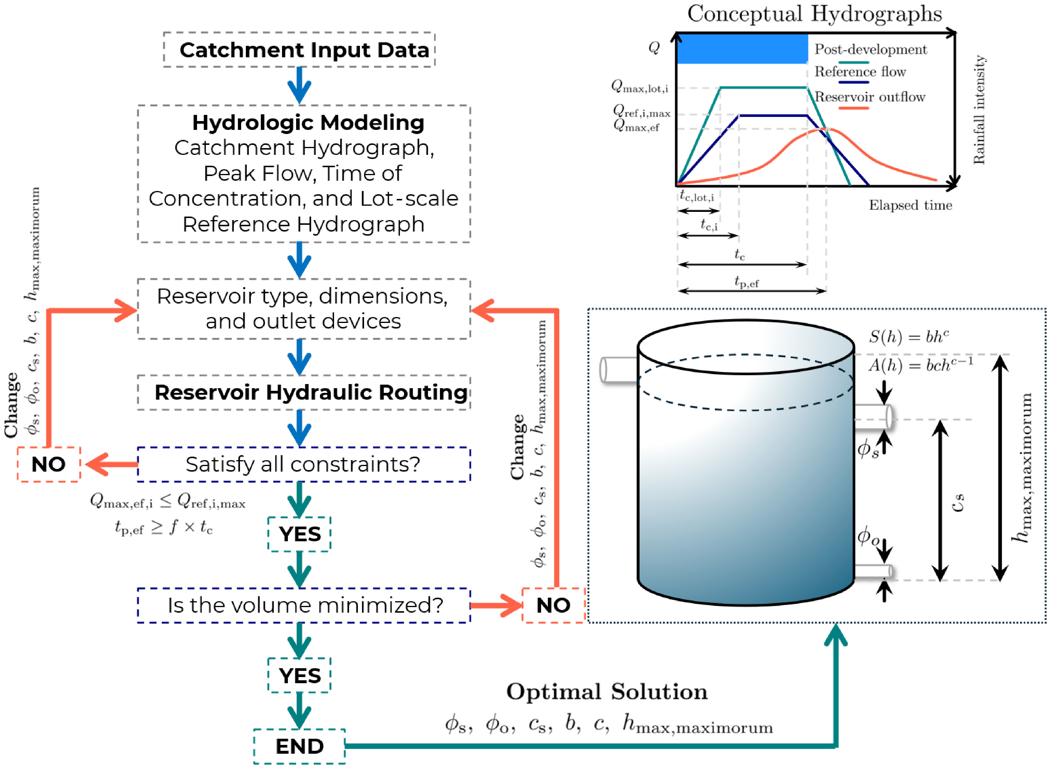
Regarding the emergency spillway, it is possible to use a rectangular shape (Francis type) for relatively larger lot-scale reservoirs or micro detention ponds. However, this is not a common solution for relatively small lots due to the magnitude of the flow rates, and circular spillways are typically used for small lot-scale reservoirs. Both types of spillways are allowed in the developed tool. Figure 3 shows a flowchart describing the steps to design a lot-scale reservoir.

Figure 3
Design of lot-scale reservoir flowchart.

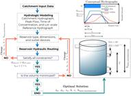
As an alternative to simulation tools such as HEC-HMS and SWMM, a dedicated design tool was developed that relies on hydrologic–hydraulic routing simulations focused on small urban catchments within condominium neighborhoods. The model follows three steps: (1) a conceptual lumped lot-scale catchment hydrological model (i.e., rational method combined with SCS-CN to estimate the runoff coefficient), (2) a conceptual reference upstream catchment lumped hydrological model that estimates the maximum reference outflow (i.e., rational method with known runoff coefficient used in the design of the drainage infrastructure), and (3) a hydraulic routing scheme solving the PULS equation to propagate the reservoir outflow.

Although typically performed manually, the design process can be formulated as an optimization problem that minimizes the reservoir volume (i.e., closely related to the reservoir cost), subject to hydrologic and hydraulic constraints. The design optimization problem is shown in Equation (21), and a conceptual model is shown in Figure 2.

$\underset{b,c}{\min }\text{V}=b\times h_{\text{max}}^{\text{c}}$

$h_{\text{max}}=\mathcal{H}\left(Q_{\text{lot},\text{i}},b,c,c_{\text{s}},{\varphi }_{\text{h}},{\varphi }_{\text{s}}\right)$

$\text{s}.\text{to}{Q}_{\text{max},\text{ef}}\le Q_{\text{ref},\text{max}}$

$t_{\text{p},\text{ef}}\ge \left(1+f\right)\times t_{\text{c},\text{i}}$ (21)

where V is the volume [L³], t_p,ef [T] is the peak time of the reservoir outflow, and f is the considered slackness in peak time compared to the reference upstream catchment, defined between 0 and + ∞, where 0 indicates that any solution with peak time at least equal to the reference catchment time of concentration is feasible. The state evolution function $\mathcal{H}$ simulates the hydrologic-hydraulic behavior of the lot-scale reservoir over the simulation time and returns the maximum water depth. Performance indicators are defined to evaluate the results and are shown in Table 1.

Table 1
Performance indicators, where V_ef is the cumulated outflow volume [L³], and V_p is the total rainfall volume over the catchment area [L³]. Variable t_c,ef indicates the reservoir effluent time of concentration, and Q_maxef the reservoir effluent peak flow.

Index	Formula	Description	Range
Time delay factor	${\eta }_1=\frac{t_{p,\text{ef}}}{{\text{t}}_{\text{c}}+{\text{ft}}_{\text{c},\text{lot}}}$	Measures the increase in the peak delay	[0, + ∞]
Peak flow factor	${\eta }_2=\frac{Q_{\text{max},\text{ef}}}{Q_{\text{ref},\text{max}}}$	Measures the ratio between inflow and outflow	[0, + ∞]
Maximum depth factor	${\eta }_3=\frac{h_{\text{max}}}{h_{\text{max},\text{maximorum}}}$	Measures the ratio between maximum depth and maximum tolerable depth	[0, 1]
Mass balance factor	${\eta }_4=1-\frac{V_{\text{ef}}}{V_{\text{p}}}$	Computes the error in volume or the storage	[0, 1]
Upstream contribution factor	${\eta }_5=\frac{(t_{\text{c},\text{i}}/A_{\text{d},\text{i}})}{\left(t_{\text{c}}/A\right)}$	Proxy for the reference contribution compared to catchment average	[0, + ∞]

The indicators η₁, η₂, η₃, η₄ and η₅ aim to explain the peak time delay indicator (i.e., the larger, the better), peak flow reduction (i.e., the smaller the better), height slackness from the maximum stipulated (i.e., the smaller the better), numerical error associated with the finite-difference scheme (i.e., the smaller the better), and the lot-scale relative contribution to the catchment (i.e., 1 indicates that the lot-scale sub-catchment contributes equally to the design made considering the whole catchment). Concerning η₅, it defines the maximum outflow a reservoir can have and compares the reference upstream catchment partial contribution to the average catchment hydrological response at the outlet. Values below unity indicate reference upstream catchments with a larger proportional contribution than the catchment average.

Excel VBA toolkit

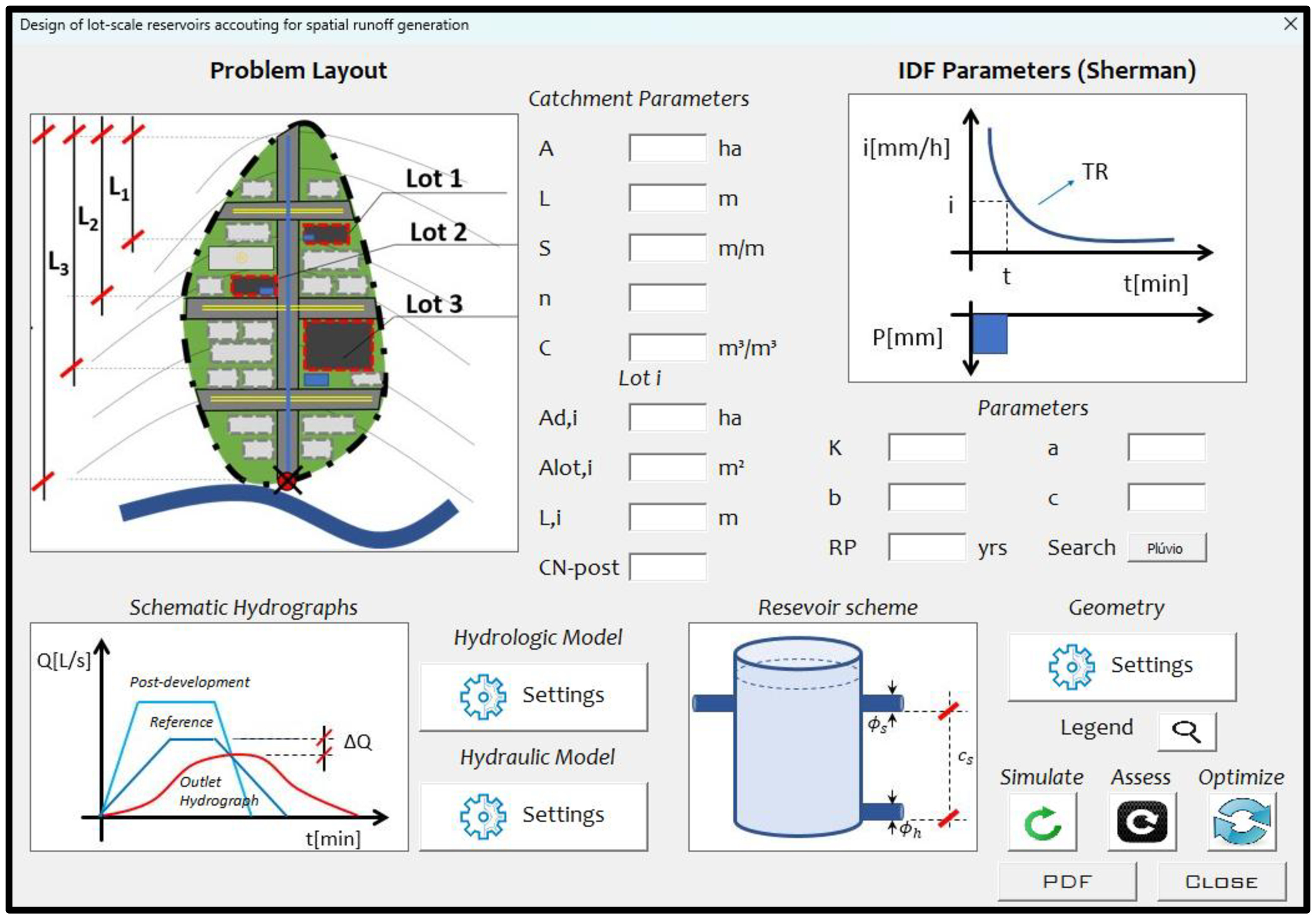
A VBA-Excel toolbox is developed to solve all equations of this paper using input data entered through guided user interfaces (GUIs). The main interfaces are presented in Figures 4, 5, and 6, where users can configure the main inputs.

Figure 4
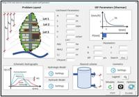
Main Guided User Interface (GUI) of the developed tool. The gray rectangular boxes in the schematic catchment represent residential or commercial lots, whereas red-dashed black boxes are fully impervious areas that require lot-scale reservoirs to mitigate excess of runoff. The main input files are the Catchment Parameters - which define the catchment and lot properties, followed by the toolboxes Hydrologic Model and Hydraulic Model Geometry input data.

Figure 5
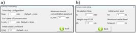
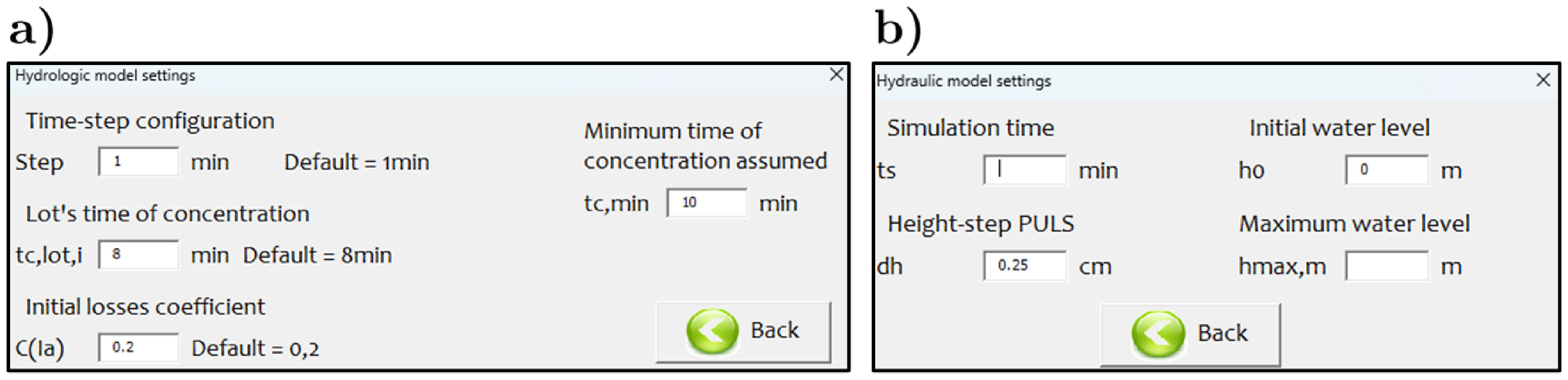
Hydrologic (a) and Hydraulic settings (b) where one can set time-step, lot-scale time of concentration, initial losses coefficient, simulation time, solver time, space discretization, initial conditions, and maximum depth.

Figure 6
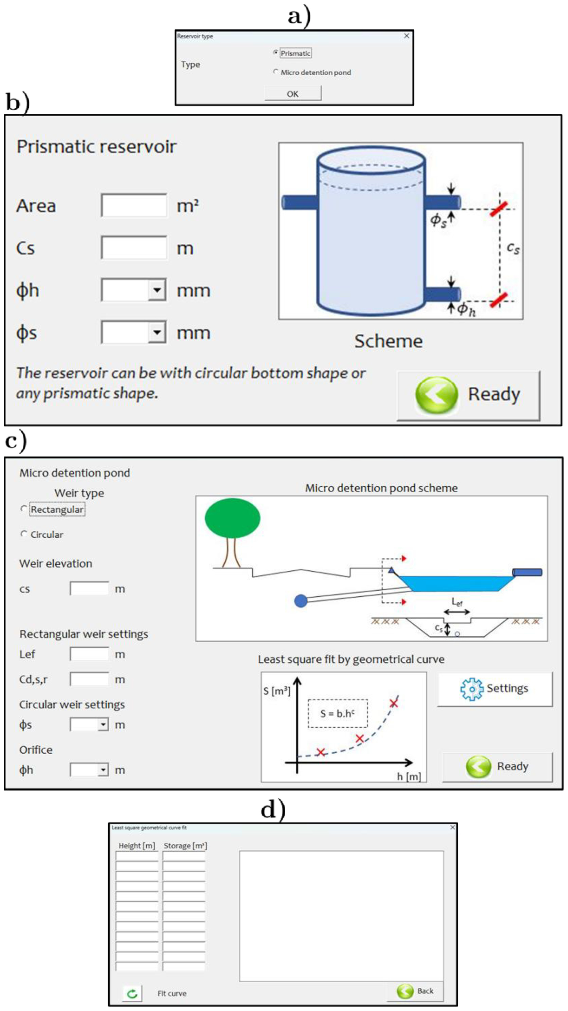
Lot-scale reservoir geometry settings, where (a) allows users to change reservoir shape, (b) shows the prismatic reservoir interface, (c) shows the micro detention pond shape, and (d) shows the tabular stage-storage input data for the micro detention design toolkit.

Numerical examples

Example 1

A condominium with a total catchment area of 3 hectares was designed for stormwater drainage using a circular pipe system dimensioned by the rational rainfall–runoff method, considering a 10-year return period and a post-development runoff coefficient of 0.8. This design assumed that, on average, individual lots would not exceed a maximum runoff coefficient of 0.8. One of the lots was later fully paved, resulting in an effective Curve Number of approximately 98. To mitigate the increase in peak discharge caused by the additional imperviousness, a lot-scale reservoir was required to control the excess runoff exceeding the pipe design capacity.

The hydrological and hydraulic parameters used in the analysis are summarized as follows. The rainfall Intensity–Duration–Frequency Sherman’s parameters were K = 7680.5, a = 0.191, b = 44.042, and c = 1.077, with a return period of 10 years. The lot is located 400 meters from the main drainage pipe, and the time of concentration was estimated using a kinematic-wave approach. The main drainage pipe is 2,000 meters long, and the mean catchment slope is 15 meters per kilometer. The Manning–Strickler roughness coefficient was assumed as $n$ = 0.020 s·m^−1/3. The reference sub-catchment area is 1.1 hectares, while the area of the individual lot is 150 square meters. The time of concentration for the lot is assumed as 8 minutes. Simulations were performed with a temporal resolution of 1 minute and a hydraulic height step of 0.25 cm to solve the PULS equations.

Example 2

For the same data used in Example 1, what should the volume of the reservoir and its outlet diameters for the orifice and spillway be, considering the same lot geometry but with double the distance downstream (L₂ = 800 m), with also double the upstream catchment area (A_d,2 = 2.2ha)?

Example 3

The new condominium management decided to build a larger lot (i.e., lot 3) in their residential area, shown in examples 1 and 2, Figure 4, with 1200 m², located at the corner of the block, at point L₃ = 1200 m with A_d3 = 2.4 ha. However, aware of the waterproofing's impacts on the receptor drainage system, they hired an engineer to design a micro detention pond to avoid further negative impacts. The designer suggested building a soccer court with reduced dimensions that could serve as a multifunction landscape, functioning as a micro detention pond during rainy periods and as a recreational area during dry ones.

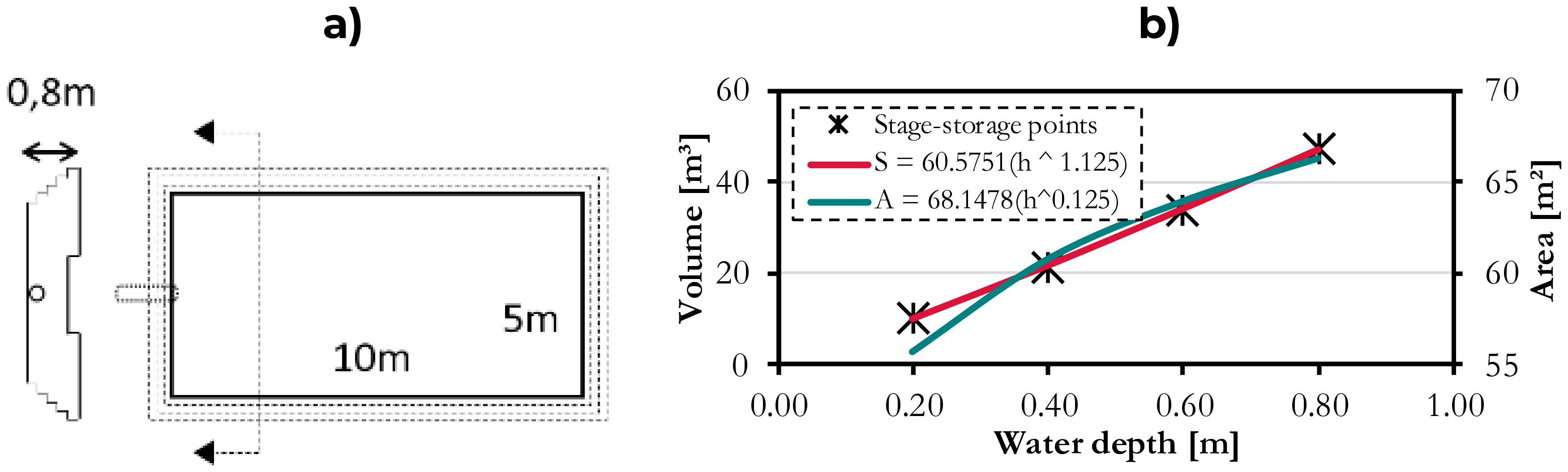
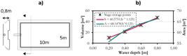
Therefore, what should be the reservoir dimensions and its hydraulic devices, considering a free rectangular spillway that must be sized for a 4% annual risk (i.e., 25-yr return period) and an orifice designed for a 10-year storm (Baptista et al., 2017). The relationship between height and volume is as follows: at 0.2 meters, the volume is 10 m³; at 0.4 meters, it is 21.23 m³; at 0.6 meters, it is 34.01 m³; and at 0.8 meters, it is 47.64 m³. These ordinates are then used to derive a closed-form expression for the stage-area-volume relationships. A schematic of the reservoir and the fitness of the stage-area-volume relationships is shown in Figure 7.

Figure 7
(a) Reservoir schematics plan view and (b) least-square stage-storage-area fit.

RESULTS

Example 1

This numerical exercise represents the typical reservoir design for a specific lot. Results are organized for the Hydrological and Hydraulic models. Results in Figure 7 summarize the hydrologic and hydraulic routing of the design problem as follows:

Hydrological model

All calculations are performed using the available spreadsheet. The calculation report, presented in the supplemental material for reference, follows the step-by-step routine shown in this paper. This first example contains all the detailed expressions to solve the hydrologic-hydraulic system of equations. The other examples will provide summaries of the results presented herein.

1. Catchment outlet time of concentration

Combining Equations (5) and (4), with 4 iterations, one can obtain ${\text{t}}_{\text{c}}=35\text{min}$.

1. Lot reference catchment time of concentration

Combining Equation (5) and Equation (4), with 4 iterations, one can obtain ${\text{t}}_{\text{c}\mathrm{,1}}=11\text{min}$.

1. Critical rainfall rate for the catchment outlet

Using Sherman IDF parameters, according to Equation (22), the rainfall intensity is:

$i=\frac{K\times {\text{RP}}^a}{{\left(b+t_{\text{d}}\right)}^c}.$ (22)

By assuming the time of concentration as the rainfall duration, one can obtain the design rainfall intensity $\text{i}=108\text{mm}/\text{h}$.

1. The maximum catchment outlet flow rate using Equation (1) results in ${\text{Q}}_{\text{max}}=718\text{L}/\text{s}$.

2. The maximum lot reference catchment flow rate using Equation (2) results in ${\text{Q}}_{\text{max}\mathrm{,1}}=226\text{L}/\text{s}$.

With the time of concentration of the catchment and the lot reference catchment maximum peak discharge, one can obtain the catchment hydrograph, shown in Figure 8.

Figure 8
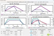
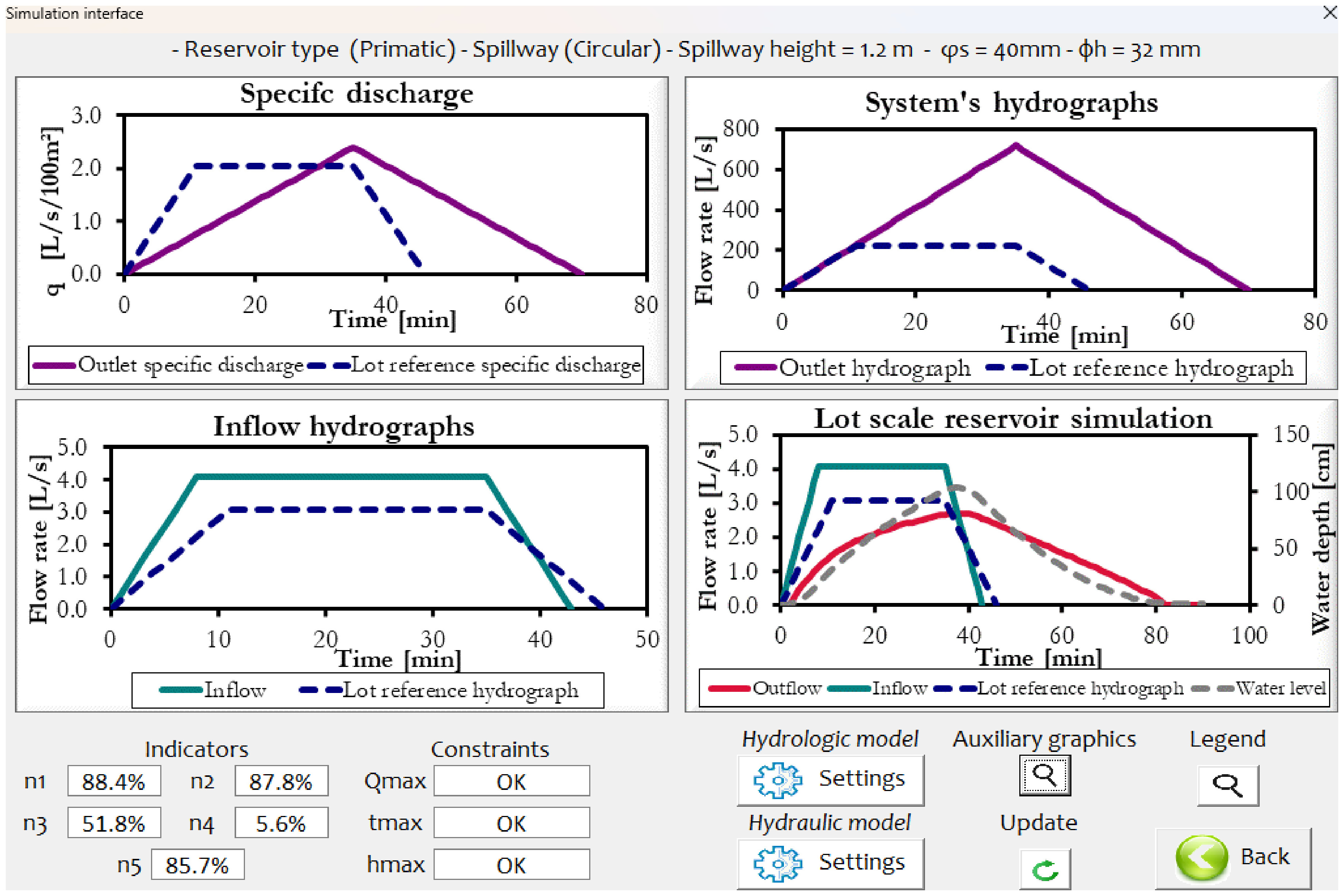
Simulation results of Example 1. At the top header, the current tested solution is indicated. The performance indicators are shown in the bottom left, and the model constraints of maximum outflow, minimum time to peak, and maximum water depth are satisfied in this example. In the tool, users can also adjust hydrologic and hydraulic parameters and visualize PULS auxiliary graphics to solve the mass balance equations.

1. Specific reference flow rate, according to Equation (3) ${\text{q}}_{\text{max}\mathrm{,1}}=205\text{L}/\text{s}/\text{ha}$

The specific inflow hydrograph is shown in Figure 8.

Figure 8 indicates that the lot reference catchment has a higher reference contribution compared to the catchment average contribution (see the specific discharge plot). This result is due to the non-linearity between the time of concentration with L and the uneven increase of area with L from the catchment hypsometry. The specific flow discharge, according to Equation (6), can be obtained as $Q_{\text{ref}\mathrm{,1,}\text{max}}=3.08\text{L}/\text{s}$.

1. Runoff coefficient:

From Equation (7), the soil storage capacity is $S^c=5.2\text{mm}$. From Eq. (8), adopting the initial losses coefficient equals 0.2, the initial abstraction is estimated as $I_{\text{a}}=1.03\text{mm}$. As the rainfall duration is 35 min, the cumulated rainfall depth is $P\left(35\right)=\frac{108\times 35}{60}=63\text{mm}$. Thus, the effective rainfall is given by Eq. (9) $P_{\text{ef}}=57\text{mm}$. Hence, the runoff coefficient can be estimated using Equation (10) results in $C_{\text{i}}=57/63=0.91$. As the lot’s runoff coefficient is higher than 0.8, it is necessary to use a lot-scale reservoir to mitigate the waterproofing impact.

1. Maximum lot’s inflow:

Using Equation (11), one can obtain $Q_{\text{max},\text{lot},\text{i}}=4.07\text{L}/\text{s}$.

1. Inflow hydrograph

The inflow hydrograph peaks at t_c,lot,1 = 4.07 L/s, remaining constant until the catchment time of concentration. Figure 8 shows the inflow hydrograph compared with the reference one. Once the inflow hydrograph at the lot-scale reservoir is defined, the hydraulic routing procedure begins.

Hydraulic routing

1. Initial conception

To ensure feasibility in the real world, a few construction constraints will be fixed to the reservoir geometry. The maximum depth constraint of $h_{\text{max}}\le h_{\text{max},\text{maximorum}}=1.5\text{m}$ is assumed, and the spillway elevation is fixed in $c_{\text{s}}=1.2\text{m}$.

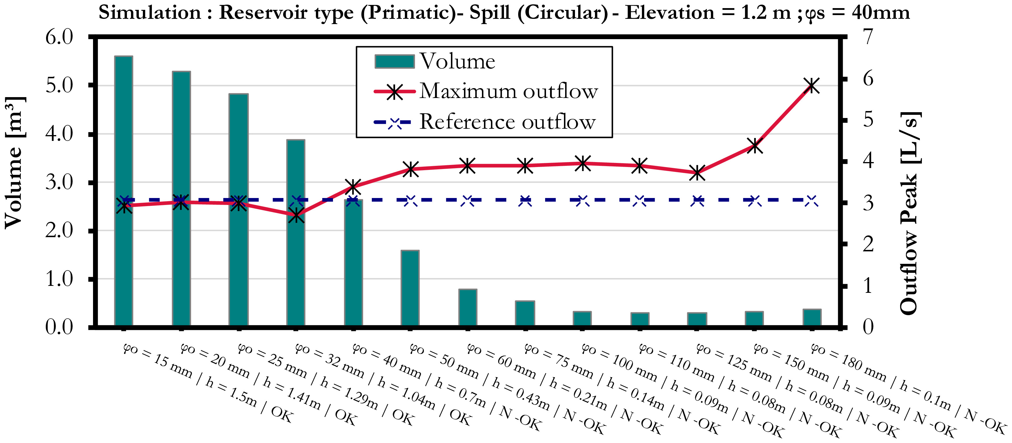
As the first attempt, one can adopt the outlet circular spillway diameter as 40 mm and consider a prismatic reservoir with 1.5 m x 2.5 m, therefore b = 3.75 m² and c = 1, according to Equation (15). Figure 9 shows the orifice diameter assessment by clicking on Assess at the main user interface from Figure 3. The analysis presented in Figure 9 shows a decision-space exploration of the orifice possibilities (i.e., given the available commercial diameters available) for a fixed spillway and reservoir surface area configuration. Figure 9 shows that a 40 mm orifice diameter requires a lower volume than a 32 mm orifice, but has a higher maximum outflow than the reference outflow. In addition, the 15 mm orifice diameter does not result in lower outflow because both the orifice and the spillway are required to convey the inflow without overflow.

Figure 9
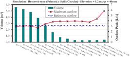
Outlet orifice diameter Monte-Carlo analysis, where all feasible internal diameters are tested to identify the minimum volume that attends the maximum flow discharge and peak time constraints.

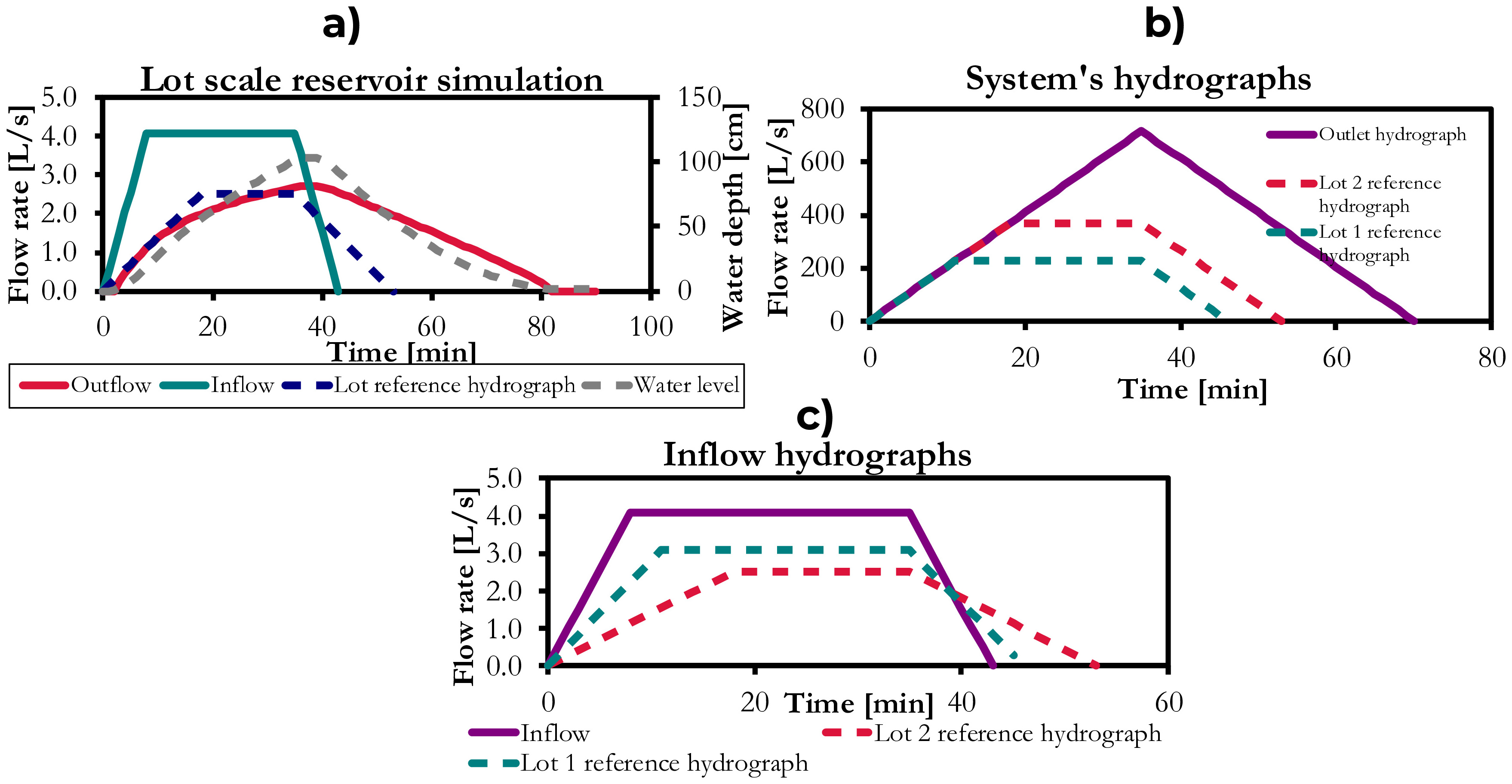
Figure 10 (a) shows the inflow and outflow lot’s hydrograph using a 32 mm orifice diameter, indicating a smaller outflow peak, delayed peak time, and avoidance of the maximum allowable design depth.

Figure 10
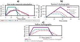
(a) Inflow, outflow, and water level in the reservoir for Example 1 results, (b) System’s hydrographs, and (c) Inflow and reference hydrographs for lots 1 and 2.

The performance indicators for this simulation are as follows: η₁ is 88.4%, η₂ is 87.8%, η₃ is 69.0%, η₄ is 5.6%, and η₅ is 85.7%, as shown in Figure 8.

Example 2

In this example, a 100% increase is observed in the reference catchment and at the lot's position. Although the area and the length doubled, the reference outflow did not double, showing the non-linearity of the time of concentration with catchment properties, even though the same roughness coefficient was assumed. These changes impact the reference catchment inflow hydrograph and require different designs for the reservoirs.

Hydrologic model

All steps of Example 1 for the hydrological modeling are solved and summarized in Table 2. It is observed that Lot 2's upstream contribution factor is 18.4% lower than Lot 1's because η₅ is 70%. In other words, the specific discharges differ primarily because of the nonlinearity in the time of concentration. Therefore, the maximum reference flow differs, even though the lots have the same area and land use. Because of this, it is necessary to have stricter control of the outlet discharge.

Table 2
Hydrologic results for example 2.

Variable	Value		Units	Variable	Value		Units
t c	35	min		Sc	5.18	mm
t ci	18	min		I a	1.04	mm
Q max	718.3	L/s		Pef(35)	57.03	mm
Q max,i	369.4	L/s		C i	0.91	m3/m3
q max,i	167.9	L/s/ha		Q max,lot,i	4.07	L/s
Q ref,i,max	2.52	L/s		η 5	70%

Comparing the inflow and the reference hydrographs for lots 1 and 2, different reference inflows for the same inflow are observed because they have the same post-urbanization but different positions and upstream areas. Figure 10 (b)-(c) shows the inflow and reference hydrograph comparison between lots 1 and 2.

Hydraulic model

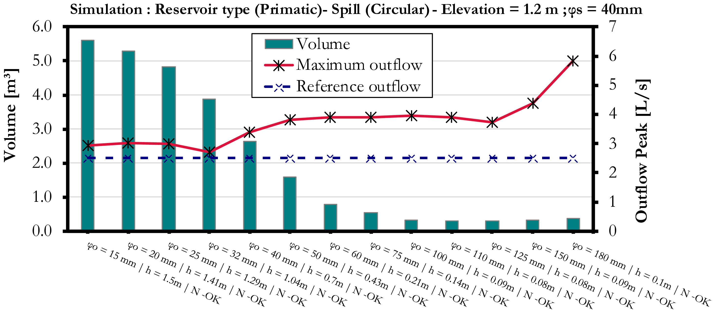
To compare the results, it is assumed that the same reservoir conditions are used for the design in Example 1. Using the same surface area for the reservoir (b = 3.75 m² and c = 1) and the same circular spill, the sensitivity analysis of the orifice diameter is shown in Figure 11.

Figure 11
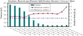
Lot’s 2 reservoir orifice assessment showing the performance of different orifice configurations for the same overall design of Example 1, which consisted of a circular spillway 1.2 m from the bottom with a 40 mm diameter and the reservoir with a 3.75 m.

From Figure 11, none of the commercial diameters tested presented feasible solutions with flows smaller than the reference flow discharge. Therefore, some decision variables in the objective function given by Equation (21) should be changed. One option with limited construction impact is to increase the spillway elevation by 10 cm, providing more storage capacity for runoff in the reservoir. This solution is feasible for a 32 mm orifice diameter, resulting in a 5.02 m³ reservoir for the 40 mm spillway.

Another approach to the problem is to decrease the spillway diameter to diminish the outflow peak, trading off with more retaining volume and hydraulic head in the hydraulic devices. For that, a search algorithm can be used to assess each orifice and spillway diameter combination, returning the solutions in tabular or graphical form. This algorithm is followed by providing a 1 x 1 combination of all possible orifice and spillway commercial diameters.

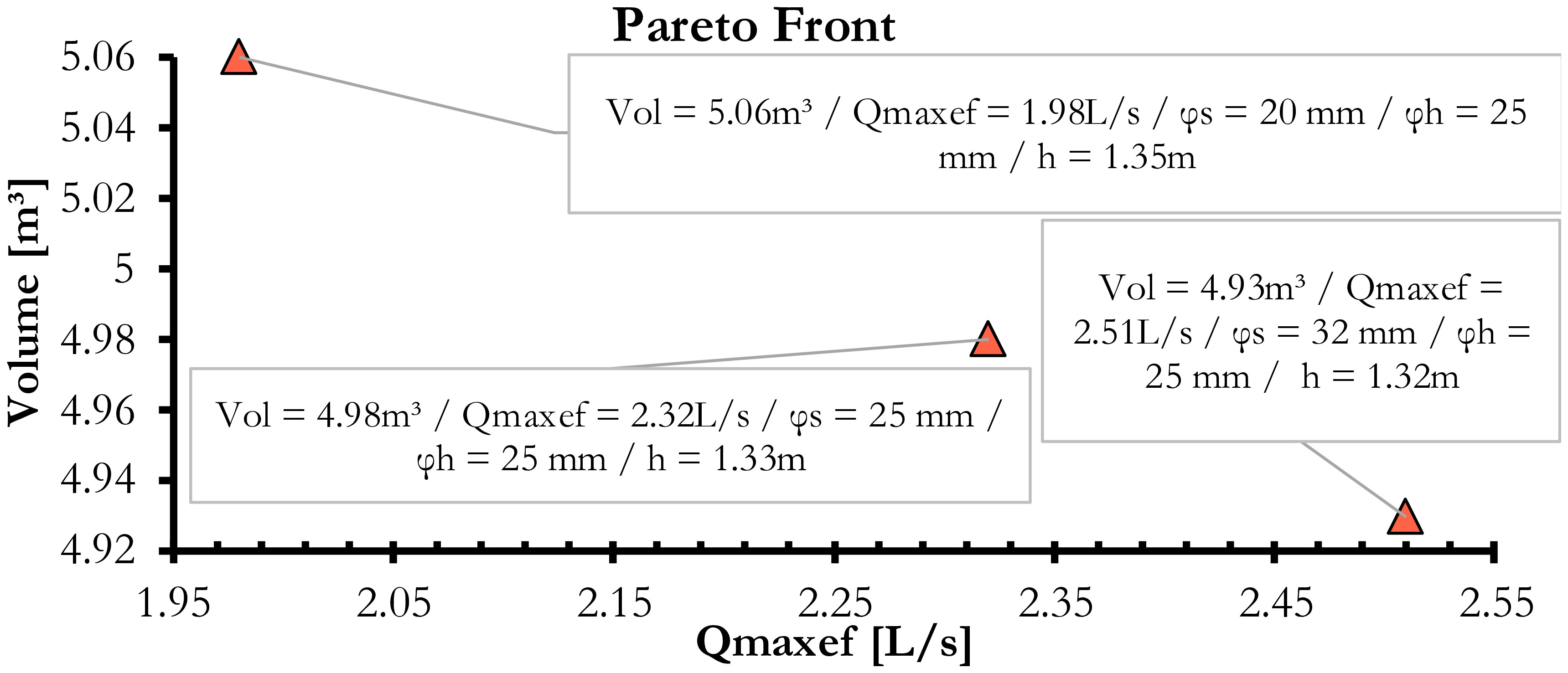
The trivial solution given by the algorithm that seeks the minimum volume satisfying the outflow constraints is to use an orifice diameter that satisfies the constraints without requiring the spillway, and therefore with a height lower than c_s. However, sometimes its diameter is not commercial, so it’s necessary to use a multiple-outlet combination to satisfy the constraints and ensure the problem's feasibility. In the spreadsheet, this algorithm can be used by clicking on optimize (see Figure 4). Figure 12 shows the Pareto front aiming to minimize the volume and the outflow, indicating three possible solutions given the available commercial diameters.

Figure 12
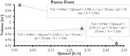
Pareto Front of non-dominated solutions when comparing reservoir volume with the maximum outflow.

The performance indicators for example 2 are as follows: η₁ = 90.7%, η₂ = 99.5%, η₃ = 87.7%, η₄ = 6.9%, and η₅ = 70.1%.

Therefore, comparing both designed reservoirs with the same area, post-urbanization showed that different volumes and hydraulic devices were needed to mitigate post-urbanization impacts on the receptor water drainage system. This was mainly due to variation in η₅ caused by the non-linearity in the time-concentration relationship. Another alternative to changing η₅ would be to change the upstream catchment area unevenly with distance along the main channel network. The comparison of results from examples 1 and 2 is shown in Table 3.

Table 3
Comparison between reservoirs of example 1 and 2, where Vol represents the minimum volume.

Lot	A d,i	A ,lot,i	L i	Volume	φ h	φ s	η 5
	[ha]	[m2]	[m]	[m3]	mm	mm	%
1	1.1	150	800	3.87	40	40	85.7
2	2.2	150	400	4.93	32	32	70.1

Example 3

Hydrologic Model for the 10-yr storm

The summary of the hydrologic modeling outputs is given in Table 4.

Table 4
Hydrologic model results for example 3 for the 10-yr and 25-yr storms. Note that, unlike empirical geometry-based time of concentration formulations, the time of concentration decreased with the increase in return period.

10-yr storm
Variable	Value		Units	Variable	Value	Units
t c	35	min		Sc	5.18	mm
t ci	24	min		I a	1.04	mm
Q max	718.3	L/s		Pef(35)	57.03	mm
Q max,i	492.5	L/s		C i	0.91	m3/m3
q max,i	205.2	L/s/ha		Q max,lot,i	21.73	L/s
Q ref,i,max	16.42	L/s		η 5	86%
25-yr storm
Variable	Value	Units		Variable	Value	Units
t c	32	min		S	5.18	mm
t ci	22	min		I a	1.04	mm
Q max	892.1	L/s		Pef(32)	65.50	mm
Q max,i	613.3	L/s		C i	0.92	m3/m3
q max,i	255.5	L/s/ha		Q max,lot,i	40.94	L/s
Q ref,i,max	30.67	L/s		η 5	86%

Hydraulic Model for the 10-yr storm

1. Reservoir sizing for a 10-yr storm or 10% annual risk

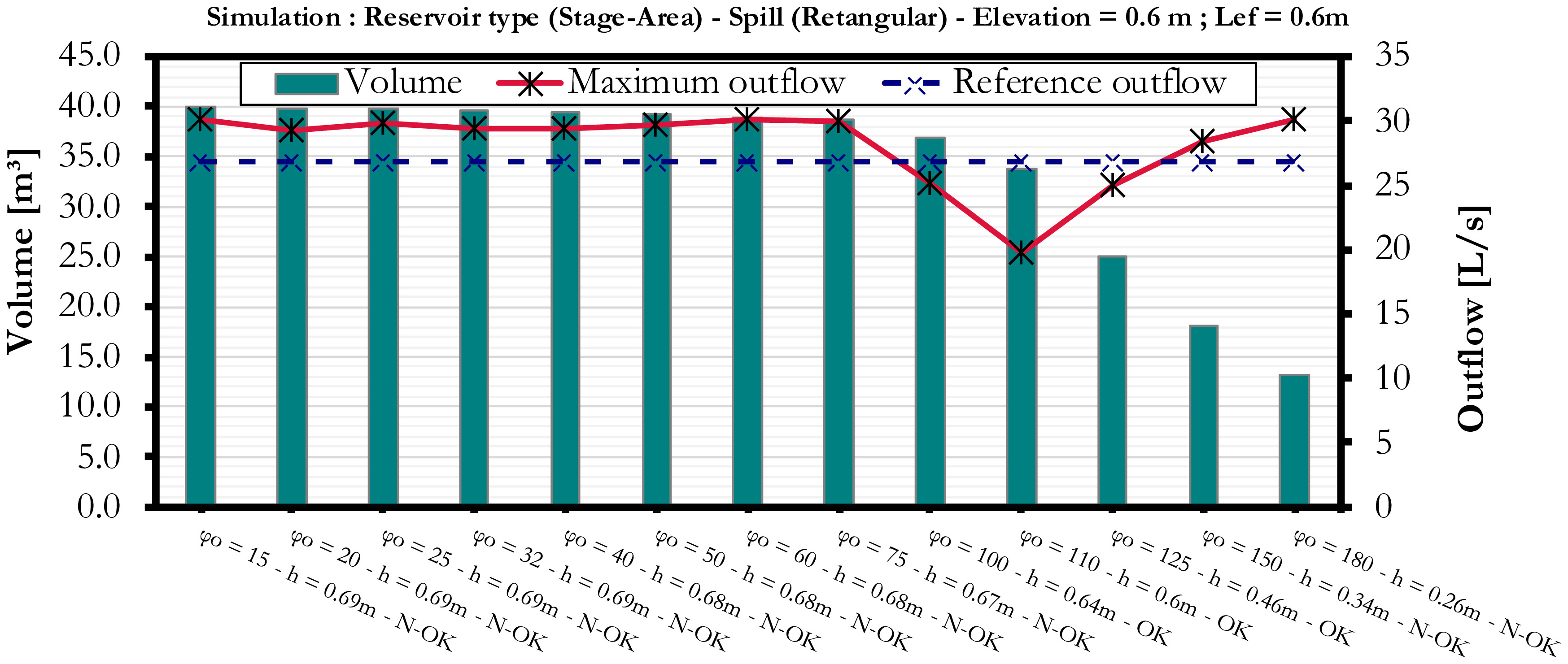
The design phase is performed in two phases. The first one aims to find the smallest volume, among the available commercial orifice diameters, that properly mitigates the inflow hydrograph by generating an outflow peak smaller than the reference flow while avoiding spillway flow. For the spillway design, one can assume an effective length (L_ef = 0.6 m) at an elevation of 0.6 m (c_s = 0.6 m) from the bottom, allowing 20 cm of hydraulic head available for the 25-year storm, which the spillway will be tested further in the analysis. With this geometry, the maximum spillway outflow is 98 L/s, using a 1.83 discharge coefficient, which is greater than the maximum inflow discharge of 21.73 L/s and hence would avoid overtopping for the 10-yr event. To ensure real-world constraints, only designs that satisfy ${\text{h}}_{\text{max}\mathrm{,3}}\le {\text{h}}_{\text{max},\text{maximorum}\mathrm{,3}}=0.8\text{m}$ are considered. Figure 13 shows the orifice outflow assessment for example 3.

Figure 13
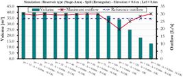
Orifice outflow assessment for example 3 – the micro detention pond – for a 10-yr storm event focusing on evaluating the orifice capacity while avoiding spillway flow.

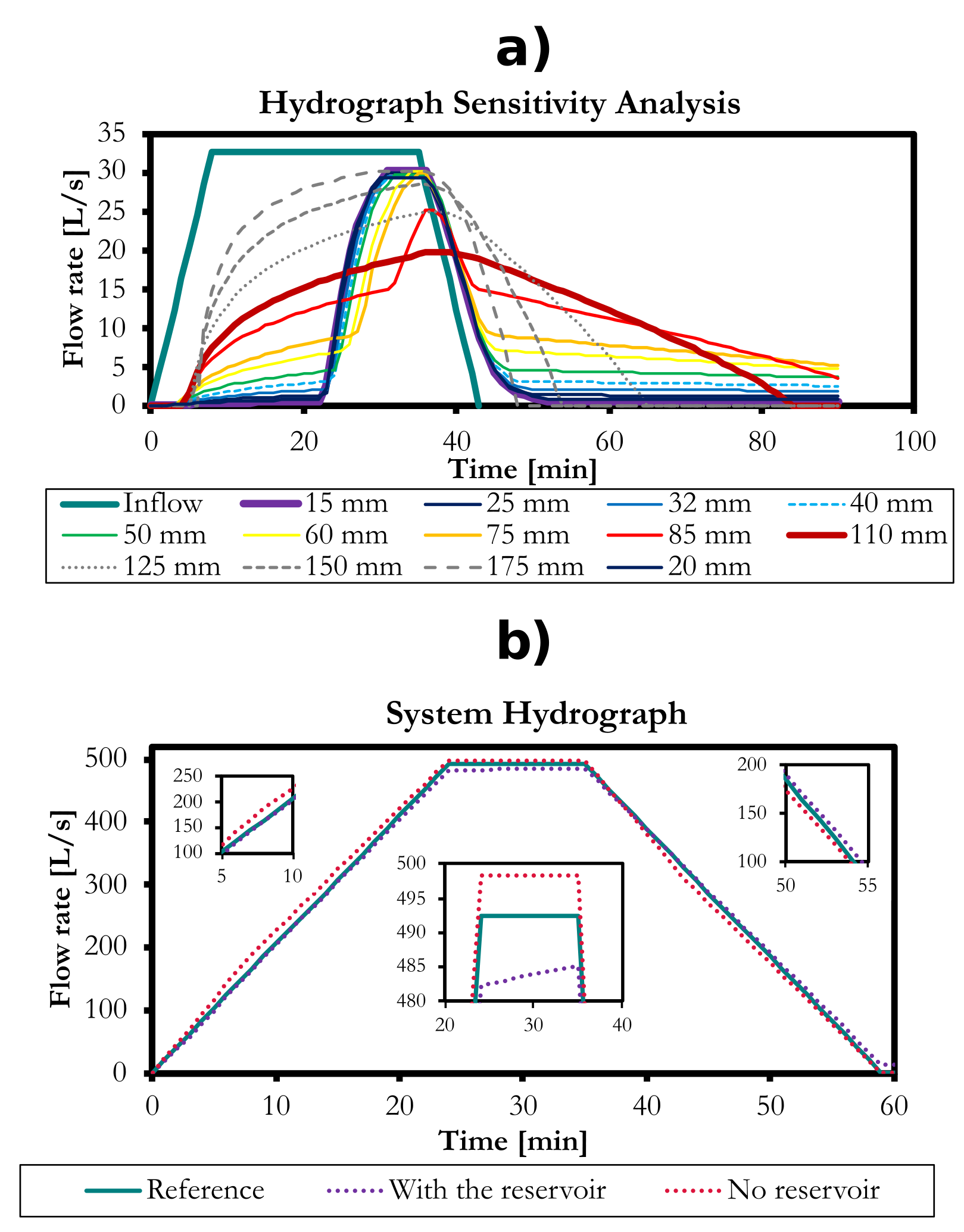
Therefore, in this initial assessment, for the rectangular weir, the unique solution is to use 110 mm as the nominal diameter of the outlet orifice. Figure 14 shows the hydrographs for each orifice diameter.

Figure 14
Outflow hydrograph sensitivity analysis where the 110 mm diameter is the optimal solution for the 10-yr design (a), and the effect of the reservoir dynamics on the lot reference hydrograph (b).

Figure 14(a) shows that a 110 mm orifice diameter is the unique commercial solution that does not use the spillway for a 10-yr storm. The 125 mm-diameter unit, although it produces a smaller volume, has a larger outflow peak due to its larger orifice capacity (see Figure 14(a)). The performance indicators for this example are: η₁ = 88.4%, η₂ = 80.2%, η₃ = 39.7%, η₄ = 12.4%, and η₅ = 85.7%.

The impact on the receptor drainage system is shown in Figure 14 (b). It is observed that there is a reduction in the peak flow and an increase in the peak time using the micro detention pond, even though its drainage area represents only 4% of the total catchment area, and the runoff coefficient ranges from 0.8 (pre-waterproofing) to 0.91 (after waterproofing of the lot). There is a 20% reduction in the outflow compared with the reference outflow at the lot-scale and a 1.05% reduction in the peak flow in the receptor drainage system using the micro detention pond. It is important to note that the system was designed not to increase peak flow or decrease peak time, and therefore, the objective was satisfied. Although the results might seem modest from the whole catchment standpoint, for the lot-scale view, not only were the flows reduced to the required maximum flow, but the reservoir provided even a larger flow mitigation (e.g., in theory, matching exactly the reference outflow would be desired, but due to limits on the commercial diameters, this is hardly achieved). In real-world catchments, results like those presented in this example are integrated across the catchment domain, ultimately leading to larger reductions at the catchment outlet when reservoirs are properly designed.

Simulation for a 25-yr storm event

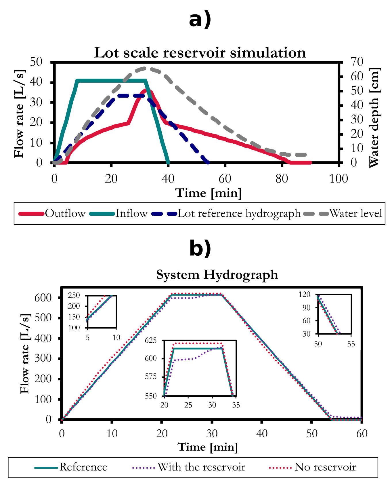
Using the same geometric project conditions for the orifice design, one can obtain the 25-yr hydrograph shown in Figure 15 (a). A summary of the hydrologic results is presented in Table 4. A peak flow increase is observed when the spillway is used, due to its greater hydraulic capacity. Figure 15 (b) shows the reservoir impact on the receptor water drainage system. A 1% increase in peak flow is observed at the reservoir for a lot area representing 4% of the catchment area. In this sense, its impact from a 25-year storm is not very significant, as the spillway for this storm ensures overtopping security, with a maximum water level of 0.66 m, below the maximum permitted level of 0.80 m. More importantly, the time during which the flow exceeded the reference flow is minimal, and a quite substantial flow mitigation is evident in Figure 15, in the inset hydrograph near the peak.

Figure 15
Hydrographs for a 25-yr-storm, where (a) shows the reservoir effects (it was designed for a 10-yr return period), whereas (b) shows the catchment-scale effect of the reservoir. Red dashed lines in (b) show the outlet hydrograph considering the waterproofing in the lot area without LID implementation.

DISCUSSION

The design of lot-scale reservoirs is still commonly approached in isolation from the broader hydrological behavior of the catchment in which they are embedded. This fragmented approach, often guided solely by local imperviousness or lot area, ignores the spatial heterogeneity of runoff generation within the catchment. As a result, "one-size-fits-all" design practices—where a fixed specific discharge or reference flow is applied uniformly—can lead to unintended consequences. Chief among these is the convolution of peak outflows: even when individual reservoirs appear compliant locally, their collective discharge can align with catchment peak flows, potentially exacerbating downstream flooding (Baptista et al., 2017).

This paper highlights the non-linear relationship between a lot’s upstream hydrological context (e.g., contributing area, time of concentration, and spatial distance along the channel network) and the outflow that its reservoir should be permitted to release in a simple, comprehensive fashion. Conventional models that neglect this relationship oversimplify the behavior of urban catchments, which are often complex mosaics of land use, topography, and urban infrastructure.

The methodology proposed in this study addresses this challenge by introducing a catchment-aware reservoir design approach that remains accessible to practitioners. By leveraging well-known models—the Rational Method, SCS–CN, and PULS—within a simplified but integrated spreadsheet-based tool, this study demonstrates that runoff generation spatial variability can be accounted for without requiring advanced software or complex simulations. The model requires only a limited number of inputs—such as rainfall IDF parameters, land-cover data represented by runoff or CN coefficients, and basic catchment characteristics to compute time of concentration—making it feasible for use in both new developments and retrofit scenarios.

Importantly, the tool emphasizes comparative hydrologic performance, ensuring that a reservoir does not exceed a reference outflow or deliver it before the catchment’s critical time to peak. As shown in the examples, even lots with identical geometries and imperviousness can demand very different reservoir volumes and outlet configurations depending on their position in the catchment and their upstream catchment hydrologic contributions.

This contributes to the broader discussion around localized or decentralized stormwater management. While decentralized infrastructure is often promoted for its modularity and flexibility, its effectiveness is significantly enhanced when local interventions are informed by upstream and downstream dynamics (Baptista et al., 2017).

Existing lot-scale reservoir and on-site detention (OSD) methods generally rely either on simplified analytical formulations—such as Tucci (1997), Silveira & Goldenfum (2007), and Dornelles et al. (2010)—or on computationally intensive hydrologic–hydraulic simulations like those of Beecham et al. (2005) and Todeschini et al. (2012). Analytical models offer transparency and ease of application but assume constant allowable discharges, steady outflow behavior, or generic hydrograph shapes, neglecting how upstream contributing area, non-linear time-of-concentration effects, and spatial position within the drainage network influence peak flow magnitude and timing. Simulation-based approaches capture dynamic routing but require specialized software, detailed parameterization, and are rarely used in regulatory design due to their complexity. Crucially, none of the existing frameworks explicitly links the allowable lot-scale outflow to the catchment-scale hydrologic response, leaving designs vulnerable to unintended peak synchronization. The model developed in this study addresses these gaps by combining the simplicity of analytical methods with a catchment-aware reference hydrograph, derived from upstream area and kinematic-wave travel time, and by using Rational + SCS–CN runoff estimation with PULS routing to enforce both maximum outflow and minimum time-to-peak constraints. This integration provides a practical yet hydrologically consistent design strategy that both critiques and advances existing approaches, enabling lot-scale interventions to operate coherently within catchment-scale flood mitigation objectives.

Although intended to aid the design of lot-scale reservoirs, the hydrological and hydraulic modeling in the tool can be used for other applications. Examples vary from (i) propagate hydrographs in large pool-leveled detention ponds, (ii) simulate lined LID systems such as bioretention or green roofs by considering a media porosity in the flow propagation dynamics, and (iii) be used as a teaching and pragmatic tool for understanding basic concepts as time of concentration, runoff generation, and flow propagation in reservoirs at graduate and undergraduate levels.

Model limitations

Some important limitations of the current framework should be clearly acknowledged. The model assumes that the time of concentration is calculated only along the longitudinal axis of the main drainage channel, using a kinematic-wave approximation of the shallow-water equations for a plane with a known slope and roughness (Akan, 1993). This implies that lateral travel distances from the main channel (i.e., hillslope positions connecting to the main channel) are not accounted for in the computation of the time of concentration, potentially underestimating real-world flow pathways. To improve this, future versions of the model could incorporate hillslope width functions (e.g., Yang et al., 2002) or a more robust approach to compute travel time, not only for the main channel but also for tributaries and for the sheet flow time to enter the channel. This can be achieved quite simply at the spreadsheet level by using the recommended SCS-CN time-of-concentration computation that considers different flow phases (Vasconcelos et al., 2025), however would require more data.

As a design tool, the fundamental limitations of design problems also apply, such as the rainfall spatio-temporal invariant distributions applied to the rational method, as well as the effects of soil initial conditions in the catchment and in the lot (Gomes Junior et al., 2025). These certainly play an important role, and investigating their effects on the design of lot-scale reservoirs is a topic for further research.

Additionally, integrating GIS tools could automate the extraction of key parameters, such as upstream contributing area and channel distance, further enhancing model usability and scalability. The use of readily available digital terrain models to determine chainage distances, coupled with a robust formula to estimate travel times, would likely improve modeling results at the cost of greater complexity for users or the need for additional GIS software. Future research should explore how this approach can be embedded into regulatory frameworks or drainage codes, replacing arbitrary thresholds with hydrologically justified constraints that evolve with changes in land use and climate. To this end, comparisons of the developed approach with existing one-size-fits-all solutions typically established in drainage codes are warranted (Dias et al., 2025). It would also be valuable to explore how this model performs under multi-lot or distributed scenarios—where spatial coordination among reservoirs could further reduce cumulative peak flows and optimize catchment-scale flood mitigation.

CONCLUSIONS

This study presents a practical hydrologically-consistent methodological framework for the hydrologic-hydraulic design of lot-scale low-impact development (LID) systems, with an emphasis on micro-reservoirs and detention ponds. The approach advances conventional practices by incorporating upstream and catchment-scale hydrological characteristics—such as terrain roughness, hypsometry, infiltration potential, and spatial position relative to the drainage network—into the local reservoir design process. This integration enables the determination of a reference maximum outflow that a lot-scale system must not exceed, ensuring compatibility with downstream drainage infrastructure.

The proposed methodology challenges the traditional assumption of spatially uniform pre-development-specific discharges, highlighting the non-linear relationship between a lot’s hydrological influence and its position within the catchment by accounting for uneven runoff generation. By reversing the standard design flow—from lot to outlet—and instead beginning from the downstream system constraints, the method ensures that additional imperviousness at the lot level can be mitigated through context-sensitive reservoir design, without increasing peak discharges at the catchment outlet.

A lumped modeling approach was adopted, combining the Rational Method for runoff estimation, the SCS-CN method for abstraction losses, and the PULS method for hydraulic routing. These models were integrated into a computational tool developed in Microsoft Excel with VBA scripting, facilitating practical application through guided user interfaces. The tool allows for sensitivity analysis and optimization based on performance criteria, including peak flow attenuation, delay of time to peak, mass balance, and compliance with maximum allowable depth.

Three case studies were employed to validate the methodology under varying spatial and hydrological conditions. Results demonstrate that lots with identical geometric and land use characteristics may require substantially different reservoir volumes and outlet structures when their upstream catchment contributions differ. In particular, the third case study demonstrated the feasibility of implementing multifunctional micro-detention ponds within urban landscapes, illustrating the potential for integrating hydraulic performance with urban design.

Despite the utility of the framework, certain limitations remain. The current implementation assumes that the time of concentration is calculated along the main channel's longitudinal axis, potentially neglecting lateral flow travel times. Future improvements could incorporate probabilistic hillslope-width functions and automated GIS-based extraction of catchment characteristics. In addition, the cumulative effect of multiple reservoirs designed with the method proposed here, and their influence at the catchment outlet, should be investigated in future studies that contrast traditional design approaches with the one developed in this paper.

DATA AVAILABILITY STATEMENT

Research data is available in the body of the article. All code and software are available in an open repository at https://github.com/marcusnobrega-eng/LotScaleReservoir.

ACKNOWLEDGEMENTS

The main author acknowledges Dr. Eduardo Mario Mendiondo, Dr. Luisa Fernanda Ribeiro Reis, and Dr. Rodrigo de Melo Porto for their insightful conversations and comments about the model, which led to fundamental advances in the developed framework.

REFERENCES

• Akan, O. A. (1993). Urban stormwater hydrology: a guide to engineering calculations Boca Raton: CRC Press.
• Baptista, M. B., de Oliveira Nascimento, N., & Barraud, S. (2017). Técnicas compensatórias em drenagem urbana Belo Horizonte: Universidade Federal de Minas Gerais.
• Beecham, S., Kandasamy, J., Khiadani, M., & Trinh, D. (2005). Modelling on-site detention on a catchment-wide basis. Urban Water Journal, 2(1), 23-32.
• Bibi, T. S., Kara, K. G., Bedada, H. J., & Bededa, R. D. (2023). Application of PCSWMM for assessing the impacts of urbanization and climate changes on the efficiency of stormwater drainage systems in managing urban flooding in Robe town, Ethiopia. Journal of Hydrology. Regional Studies, 45, 101291.
• Canholi, A. (2015). Drenagem urbana e controle de enchentes São Paulo: Oficina de Textos.
• Costa, I. R. A., Coutinho, A. P., Montenegro, S. M. G. L., Rabelo, A. E. C. G. C., Santos Neto, S. M., Alves, E. M., & Antonino, A. C. D. (2020). Sensitivity of hydrodynamic parameters in the simulation of water transfer processes in a permeable pavement. RBRH, 25, e47.
• Dias, M. L., Silva, T. F. G., Drumond, P. D. P., Rosa, D. W. B., & Moura, P. (2025). Evaluating the performance of on-site stormwater detention based on the technical guidelines for developing stormwater projects in Belo Horizonte (MG, Brazil). RBRH, 30, e44.
• Dornelles, F., Tassi, R., & Goldenfum, J. A. (2010). Avaliação das técnicas de dimensionamento de reservatórios para aproveitamento de água de chuva. RBRH, 15(2), 59-68.
• Ferreira, L. T. L. M., Neves, M. G. F. P., & Souza, V. C. B. (2019). Puls method for events simulation in a lot scale bioretention device. RBRH, 24, e36.
• Fileni, F. D. M., Costa, M. E. L., & Alves, C. D. M. A. (2019). The application of LIDs in Savanna region for mitigation of flooded areas. RBRH, 24, e40.
• Gomes Junior, M. N., Giacomoni, M. H., de Macedo, M. B., do Lago, C. A. F., Brasil, J. A. T., de Oliveira, T. R. P., & Mendiondo, E. M. (2023). A modeling framework for bioretention analysis: assessing the hydrologic performance under system uncertainty. Journal of Hydrologic Engineering, 28(9), 04023025.
• Gomes Junior, M. N., Taha, A. F., Rápalo, L. M. C., Mendiondo, E. M., & Giacomoni, M. H. (2024). Real-time regulation of detention ponds via feedback control: balancing flood mitigation and water quality. Journal of Hydrology (Amsterdam), 643, 131866.
• Gomes Junior, M. N., Lago, C. A. F., & Mendiondo, E. M. (2025). A simple method for designing infiltration low impact development techniques considering effects of urbanization and climate change. RBRH, 30, e41.
• Gomes Junior, M. N., Braga, P. A., de Macedo, M. B., & Mendiondo, E. M. (2019). Análises estatísticas, visuais e não paramétricas para a otimização do ajuste de curvas IDF e construção de ábacos de projeto de obras hidráulicas: estudo de caso em São Carlos SP. Revista DAE, 69(228), 171-189.
• Kuichling, E. (1889). The relation between the rainfall and the discharge of sewers in populous districts. Transactions of the American Society of Civil Engineers, 20(1), 1-56.
• McCuen, R. H. (1998). Hydrologic design and analysis New Jersey: Prince Hall.
• Mishra, S. K., & Singh, V. P. (2013). Soil conservation service curve number (SCS-CN) methodology Berlin: Springer Science & Business Media.
• Mulvaney, T. J. (1850). On the use of self-registering rain and flood gauges. Proceedings - Institution of Civil Engineers, 4, 1-8.
• Porto, R. M. (2006). Hidráulica básica (4. ed.). São Carlos: EESC-USP.
• Prefeitura de Belo Horizonte. (2022). Instrução técnica para elaboração de estudos e projetos de drenagem urbana do município de Belo Horizonte Belo Horizonte: Prefeitura de Belo Horizonte.
• Rossman, L. A. (2010). Storm Water Management Model user’s manual, version 5.0, vol. 276 Cincinnati, OH: U.S. Environmental Protection Agency.
• São Paulo. (2007). Lei nº 12.526, de 02 de Janeiro de 2007. Estabelece normas para a contenção de enchentes e destinação de águas pluviais. Governo do Estado de São Paulo, São Paulo.
• Silveira, A. L. L. (2005). Desempenho de fórmulas de tempo de concentração em bacias urbanas e rurais. RBRH, 10(1), 5-23.
• Silveira, A. L. L., & Goldenfum, J. A. (2007). Metodologia generalizada para pré-dimensionamento de dispositivos de controle pluvial na fonte. RBRH, 12(2), 157-168.
• Tassi, R., & Villanueva, A. O. (2004). Análise do impacto dos microrreservatórios de lote nos custos de uma rede de drenagem urbana. RBRH, 9(3), 89-98.
• Todeschini, S., Papiri, S., & Ciaponi, C. (2012). Performance of stormwater detention tanks for urban drainage systems in northern Italy. Journal of Environmental Management, 101, 33-45.
• Tucci, C. E. M. (1997). Plano diretor de drenagem urbana: princípios e concepção. RBRH, 2(2), 5-12.
• Tucci, C. E. M. (2002). Gerenciamento da drenagem urbana. RBRH, 7(1), 5-27.
• Vasconcelos, J. G., Gomes Junior, M. N., Oliveira, P. T. S., Yang, D., & Fang, X. (2025). Reformulating the Rational Method considering dissimilar land use types. Journal of Irrigation and Drainage Engineering, 151(4), 04025017.
• Vietz, G. J., Walsh, C. J., & Fletcher, T. D. (2016). Urban hydrogeomorphology and the urban stream syndrome: treating the symptoms and causes of geomorphic change. Progress in Physical Geography, 40(3), 480-492.
• Walsh, C. J., Roy, A. H., Feminella, J. W., Cottingham, P. D., Groffman, P. M., & Morgan, R. P. (2005). The urban stream syndrome: current knowledge and the search for a cure. Journal of the North American Benthological Society, 24(3), 706-723.
• Yang, D., Herath, S., & Musiake, K. (2002). A hillslope-based hydrological model using catchment area and width functions. Hydrological Sciences Journal, 47(1), 49-65.

Edited by

• Editor-in-Chief:
  Adilson Pinheiro

• Associated Editor:
  Iran Eduardo Lima Neto

Publication Dates

• Publication in this collection
  10 Apr 2026
• Date of issue
  2026

History

• Received
  16 Apr 2025
• Reviewed
  26 Nov 2025
• Accepted
  13 Jan 2026