Energy efficiency in pumping systems at wastewater treatment plants: case study of the Barueri WWTP

Eficiência energética em sistemas de bombeamento em estações de tratamento de esgoto: estudo de Caso da ETE Barueri

ABSTRACT

In wastewater treatment plants, energy costs account for approximately 50% of total operating costs, mainly due to the operation of compressors and pumps. In this context, this study proposes a mathematical and computational model applied to optimize the pumping operation in wastewater treatment plant through the dynamic adjustment of variable-speed pump rotation. The model was developed based on the integration of design information and operational from Barueri Wastewater Treatment Plant, combined with numerical methods and procedures established in the technical literature for the solution of the hydraulic problem. The assessment showed a reduction on the order of 0.024 kWh/m³ in specific energy consumption among the proposed scenarios. This approach is particularly relevant in the context of Brazil’s new legal framework for sanitation, which promotes the expansion and modernization of systems nationwide and demands greater energy efficiency and operational sustainability. The developed model has a comprehensive and transferable character and can be adapted and applied to other wastewater treatment plants and related pumping systems.

Keywords:
Energy efficiency; Pumping systems; Variable-speed pumps; Numerical methods; WWTPs; Computational hydraulics

RESUMO

Em estações de tratamento de esgoto, os custos de energia representam aproximadamente 50% dos custos operacionais totais, principalmente devido à operação de compressores e bombas. Nesse contexto, este estudo propõe um modelo matemático e computacional aplicado à otimização da operação de bombeamento em estações de tratamento de esgoto por meio do ajuste dinâmico da rotação de bombas de velocidade variável. O modelo foi desenvolvido com base na integração de informações de projeto e dados operacionais da Estação de Tratamento de Esgotos de Barueri, combinados com métodos numéricos e procedimentos estabelecidos na literatura técnica para a solução do problema hidráulico. A avaliação mostrou uma redução da ordem de 0,024 kWh/m³ no consumo específico de energia entre os cenários propostos. Essa abordagem é particularmente relevante no contexto do novo marco legal do saneamento no Brasil, que promove a expansão e modernização dos sistemas em todo o país e exige maior eficiência energética e sustentabilidade operacional. O modelo desenvolvido apresenta caráter abrangente e transferível, podendo ser adaptado e aplicado a outras estações de tratamento de esgoto e a sistemas de bombeamento correlatos.

Palavras-chave:
Eficiência energética; Sistemas de recalque; Bombas de velocidade variável; Métodos numéricos; ETE; Hidráulica computacional

INTRODUCTION

The accelerated and unplanned growth of large urban centers has intensified the challenges associated with managing essential public services, requiring strategic sectors to reinvent their operational practices in order to ensure sustainable human development. In structural activities such as water supply, wastewater collection and treatment, and other utility services, conventional market dynamics do not fully apply, since regulatory frameworks, technical constraints, and social responsibilities guide and restrict managerial decisions. In the sanitation sector, long-term sustainability depends on balancing financial viability, universal service coverage, and environmental protection. In Brazil, this discussion has gained emphasis following the approval of the Brazilian Sanitation Legal Framework, established by Federal Law No. 14,026/2020 (Brasil, 2020), which expanded private-sector participation and set ambitious goals for 2033, including 99% coverage of drinking water supply and 90% wastewater collection and treatment.

However, the most recent national data indicate that wastewater treatment coverage reaches only about 56% of the population (Sistema Nacional de Informações sobre o Saneamento, 2025), as shown in Figure 1, revealing a scenario still far from the planned target and reinforcing the urgency of technical and operational advances to support sector expansion.

Figure 1
Population with Access to Sanitation Services in Brazil (2014–2021).

From an operational perspective, Wastewater Treatment Plants (WWTPs) represent a significant share of the energy consumption of sanitation systems. In Brazil, the national specific energy consumption indicator has remained practically stagnant in recent years, ranging between 0.30 and 0.33 kWh per cubic meter of treated wastewater (Figure 2), according to SNIS (Sistema Nacional de Informações sobre o Saneamento, 2025).

Figure 2
Average energy consumption per volume of wastewater treated in Brazil (kWh/m³) from 2014 to 2021.

International studies corroborate this concern: the Water Environment Federation (2002) reports that energy may account for 25% to 50% of a WWTP’s operational expenditures. While global references often present broad energy indicators for wastewater pumping, Panepinto et al. (2016) in a study to evaluate the energy efficiency of large wastewater treatment plants in Italy, provide a more explicit and detailed assessment, reporting values ranging from 0.30 to 0.73 kWh per cubic meter in European facilities. This evidence reveals a structural paradox in the Brazilian context: despite the still limited-service coverage, national energy consumption indicators are already elevated, which highlights the need to improve operational efficiency in existing systems.

The Barueri Wastewater Treatment Plant, located at Metropolitan Region of São Paulo, which serves as the case study for this research, operates using the activated sludge process – a technology widely applied in large urban centers due to its high efficiency in removing organic matter and nutrients. In systems of this nature, aeration and pumping are the most energy-intensive subsystems, making operational efficiency a strategic priority. Although the activated sludge process is more energy-intensive than alternative treatment technologies, it is capable of treating larger flow rates with superior performance. This aligns with Noyola et al. (2012), who report that approximately 58% of all wastewater treated in Latin America and the Caribbean relies on this process, reinforcing the importance of pursuing energy-optimization strategies in facilities that depend on activated sludge systems.

Within this context, optimizing energy consumption in pumping systems emerges as a concrete opportunity to reduce operational costs without compromising treatment performance or service capacity. This is closely related to the operational efficiency of hydraulic machines, for which strategies based on adjusting machine variables, particularly rotational speed, enable operation closer to the Best Efficiency Point (BEP), reducing hydraulic losses and energy consumption. Previous studies have demonstrated that variable-speed control in pumping systems leads to significant energy savings (Móller et al., 2020). For Barueri WWTP, the use of variable-speed pumps enables continuous adjustment of rotational speed as a function of the inlet well level. The control strategy consists of simulating and commanding the pumping operation to maintain the upstream reservoir at a stable operating level, thereby improving hydraulic stability and keeping pumps operating closer to their Best Efficiency Point (BEP). As a consequence, specific energy consumption, measured in kWh/m³, is reduced, and system operation becomes more stable, predictable, and sustainable.

In light of these considerations, the present study focuses on assessing how different reference water levels in the inlet well influence hydraulic behavior and daily energy consumption in the pumping system, with the goal of comparing the energy performance associated with each operating level over a 24-hour cycle.

The structure and methodological development of this work are outlined as follows. Initially, in the Materials and Methods section, the theoretical foundations governing the operation of pumping systems are established based on the energy balance between the head supplied by the pump and the head required by the hydraulic system, including static head and total head losses. In this context, the characteristic head curves of both the pump and the system are formulated and employed to determine the operating point through their intersection. Since this equilibrium condition leads to a nonlinear equation in terms of flow rate, Newton-Raphson method is applied to solve the hydraulic problem and estimate the associated specific energy consumption of pumping. Subsequently, the case study of the Barueri Wastewater Treatment Plant is presented, describing the configuration of the inlet well, the layout of the pumping system, and the main hydraulic components involved, with emphasis on the pumping stage, which constitutes the central focus of this research. The database used in the study is then detailed, comprising design information and real operational records from the plant, which support the modeling of pump characteristic curves and the characterization of the system’s hydraulic resistance.

Based on this information, different operational scenarios and rotational control strategies for variable-speed pumps are defined, enabling the assessment of how the reference level of the inlet well influences hydraulic stability and energy performance of the pumping system. Finally, the results are presented and discussed in light of specific energy consumption indicators, leading to the conclusions of the study and highlighting the applicability of the proposed approach to other wastewater treatment plants and related pumping systems.

MATERIAL AND METHODS

Pumping operation

The pumping operation in pressurized wastewater systems is governed by the balance between the energy supplied by the pump and the head demanded by the hydraulic system. The application of the First Law of Thermodynamics to internal flows leads to the operating condition:

$H_B=\Delta H+RQ²$ (1)

where $H_B$, in meters,​ is the pump head curve; $\Delta H=z_2-z_1$, also in meters, ​is the static head between the discharge channel and the inlet well; $R$, in $s^2{m}^{-5}$, is the hydraulic resistance of the system; and $Q$, in $m^3/s$, is the pumped flow rate. The left-hand side of Equation 1 represents the head provided by the pump, while the right-hand side represents the system head curve, which depends on static head and friction effects. The intersection between these curves defines the steady operating point. The validity of Equation 1, according to Walski et al. (2001) assumes a real, internal, incompressible, steady, isothermal, and homogeneous flow, with the fluid behaving as a Newtonian, which is consistent with pressurized sewage transport conditions. The head added by the pump depends on both the flow rate $Q$ and the speed ratio $\alpha$, and can be expressed as:

$H_B\left(Q,\alpha \right)={\alpha }^2{A}_H+\alpha B_{H}Q+C_{H}Q²+{\alpha }^{-1}{D}_{H}Q³+{\alpha }^{-2}{E}_H{Q}^4$ (2)

where $A_H,B_H,C_H,D_H$​ and $E_H$​ are regression coefficients. The non-dimensional rotational ratio $\alpha$, originates from the Affinity Laws, derived through dimensional analysis (White, 2011), which provide the functional similarity between pump performance and rotational speed:

$H\propto {\alpha }^2,Q\propto \alpha ,$ (3)

For variable-speed pumps, the present work adopts $0.75\le \alpha \le 1.00$, a range widely practiced by specialists in the pump industry, as excessively low speeds increase internal recirculation losses and may cause overheating of the equipment. The hydraulic resistance of the system, associated with distributed and localized head losses, is computed from:

$R=\frac{1}{2g}\left({\displaystyle \sum }_{i=1}^{NP}\frac{f_i{L}_i}{D_i{A}_i^2}+{\displaystyle \sum }_{j=1}^{NF}\frac{k_j}{A_j^{*}{}^2}\right)$ (4)

where NP is the number of pipes; NF is the number of fittings; $f$ is the non-dimensional Darcy–Weisbach friction factor, which, could be obtained from the literature equation (Porto, 2006); $L$ and $D$, both in meters, are pipe length and the internal diameter, respectively; $A$, in m², the internal cross-sectional area; $k$ the non-dimensional local head-loss coefficient, whose values may be taken from Idelchik (2007); and $A_j^{*}$, also in meters, is the upstream cross-sectional area in cases of hydraulic transitions, as defined by Tullis (1989), while the specific energy consumption (kWh/m³) associated with pumping operation is given by:

$E=\frac{\gamma H_B}{3.6\times {10}^6\eta }$ (5)

where $\gamma$ (N/m³) is the specific weight of the fluid and $\eta$ is the non-dimensional pump efficiency, obtained from its characteristic curve:

$\eta \left(Q\right)=A_{\eta }+B_{\eta }Q+C_{\eta }Q²+D_{\eta }Q³+E_{\eta }{Q}^4$ (6)

The literature does not present a consensus regarding the behavior of rotodynamic pump efficiency under variable rotational speed. Gülich (2003) indicates that efficiency is affected by Reynolds-number variations, implying a dependence of $\eta$ on the speed ratio $\alpha$. In contrast, Porto (2006) reports that such deformation is minor for engineering applications and that the efficiency curve may be treated as invariant. Considering this divergence, and aiming to avoid unnecessary model complexity, this study adopts the simplifying assumption that efficiency does not vary with rotational speed, i.e., $\eta \left(Q,\alpha \right)\approx \eta \left(Q\right)$.

By substituting Equation 2 into Equation 1, the energy balance yields a nonlinear algebraic equation in terms of the flow rate $Q$, for which no closed-form analytical solution exists. Since $\alpha$ is treated as a constant during the solution of each operating point, the problem reduces to finding the root of

$\begin{array}{l}f\left(Q,\alpha \right)={\alpha }^2{A}_H+\alpha B_{H}Q+\left(C_H-R\right)Q^2+\\ {\alpha }^{-1}{D}_H{Q}^3+{\alpha }^{-2}{E}_H{Q}^4-z_2+z_1=0\end{array}$ (7)

whose solution satisfies the hydraulic equilibrium between the pump characteristic curve and the system head curve. Because $\alpha$ is constant in this step, the derivative of $f\left(Q,\alpha \right)$ is taken only with respect to $Q$, yielding:

$f\text{'}\left(Q\right)=\frac{df\left(Q,\alpha \right)}{dQ}$ (8)

The flow rate is then computed using the Newton–Raphson iterative method (Chapra & Canale, 2011):

$Q_{n+1}=Q_n-\frac{f\left(Q_n,\alpha \right)}{f\text{'}\left(Q_n\right)}$ (9)

Convergence is ensured by selecting a physically meaningful initial guess $Q_0$​ consistent with the pump capacity, which prevents non-physical solutions and numerical divergence. After convergence, the updated values of $H_B$​, $\eta$, and $E$ represent the instantaneous hydraulic state of the pumping system.

Study case and Database

As illustrated in the schematic flow diagram provided in Figure 3, the Barueri Wastewater Treatment Plant operates based on a conventional activated sludge configuration in which raw sewage first enters the inlet well, which functions as the main hydraulic interface between the collection system and the treatment process. From this inlet well, the wastewater is conveyed through pumping systems to downstream treatment units, sequentially passing through screening and grit removal stages before entering the biological reactors and secondary clarification tanks.

Figure 3
Schematic flow diagram of the Barueri Wastewater Treatment Plant with activated sludge process.

After treatment, the effluent is discharged into the receiving water body in accordance with environmental standards. Within this overall treatment chain, the present study is specifically focused on the pumping stage – highlighted in red in Figure 3 – analyzing how the operation of variable-speed and constant-speed pumps influences the hydraulic behavior and energy performance of the system as a whole.

As illustrated in Figure 4, the sewage discharge $Q_{ef}\left(t\right)$, in m³/s, arriving at the Barueri WWTP is first conveyed to the upstream reservoir, referred to as the inlet well (IW), which has a variable water level $z_1\left(t\right)$, in meters. From this reservoir, the flow is pumped to the downstream reservoir, a discharge channel with fixed elevation $z_2=726.39m$, through four independent pumping systems operating in parallel. Each system is composed of one pump, an associated pressurized pipeline, and localized accessories (fittings), which together define the hydraulic resistance and operating head losses along the flow path. Among the four installed pumping units, three (Systems 1, 2 and 3) are equipped with variable-speed (VS) pumps, while System 4 operates at constant speed (CS), enabling a direct comparison of different pumping control philosophies under the same hydraulic boundary conditions.

Figure 4
Schematic arrangement of the Barueri WWTP pumping operation.

The database used in this study is the same employed by Nascimento (2024), consisting of design information and operational records from the Barueri Wastewater Treatment Plant. The design dataset includes the head and efficiency characteristic curves of the VS and CS pumps, which are essential for representing the hydraulic behavior of the pumping systems in mathematical form. The operational dataset, in turn, is composed of hourly measurements of the flow rates $Q_{ef}\left(t\right)$ from each pumping system and the corresponding inlet well water level $z_1\left(t\right)$. These measurements were recorded throughout September and October 2021, a period during which Pumping System 2 remained out of operation. In this interval, Systems 1 and 3 (both VS pumps) and System 4 (CS pump) remained active, making it possible to evaluate, within the same hydraulic layout, the influence of speed control on pumping performance and energy consumption.

This configuration is particularly relevant because, in variable-speed pumps, the speed ratio $\alpha$ directly modifies the head curve $H_B\left(Q,\alpha \right)$, meaning that the operating point depends simultaneously on the inlet well level $z_1$ and the applied rotational speed $\alpha$. In contrast, for the constant-speed unit ($\alpha =1$), the operating condition is uniquely defined by the intersection between the pump characteristic curve and the system head curve, depending solely on fluctuations of the inlet well level $z_1\left(t\right)$.

The characteristic curves adopted in this study – the pump head curve $H_B\left(Q,\alpha \right)$, and the pump efficiency curve $\eta \left(Q\right)$ – were previously adjusted by Nascimento (2024) and are represented in the form of Equations 2 and 6, respectively. The polynomial coefficients used in both regressions, where head is given in meters, flow rate in cubic meters per second and efficiency is non-dimensional, are presented in Table 1, consolidating the adjustment parameters employed for modeling the hydraulic performance of both variable-speed and constant-speed pumps.

Table 1
Polynomial regression coefficients for the head and efficiency curves of the constant-speed and variable-speed pumps, according to Equations 2 and 6.

	Constant-speed pump		Variable-speed pump
	$H_B\left(m\right)$	$\eta (-)$	$H_B\left(m\right)$	$\eta (-)$
$A_{H,\eta }$	52.976	0.000898	54.5	-0.00021
$B_{H,\eta }$	-5.5983	0.18834	-1.9961	0.43366
$C_{H,\eta }$	1.1839	0.010903	-0.0735	-0.06741
$D_{H,\eta }$	-0.1729	-0.00283	-0.0234	0.003933
$E_{H,\eta }$	0.0053	0	-0.0031	-0.00011

Hydraulic resistance curves

The hydraulic resistance curves describe the relationship between the system resistance $R$ and the flow rate $Q$, characterizing the global head loss behavior during pump operation. In the energy balance that governs the system, Equation 1, the resistance term $R$ is a fundamental component of the system characteristic curve, which represents the hydraulic losses and intersects the pump head curve to define the operating point. Considering the classical head loss formulation, the resistance $R$ depends on the friction losses and local losses of the system, which are functions of the Darcy–Weisbach friction factor $f$ and the local loss coefficients $k$, as described by Equation 4. Since $f$ and $k$ depend on the Reynolds number and the internal roughness of the conduit, and assuming a constant geometry – i.e., constant number of fittings and constant $L$, $D$ and $A$ – the variation in $R$ is governed only by changes in flow rate $Q$. Furthermore, by neglecting roughness growth (fouling phenomena) over the analysis period, and considering constant fluid properties, $R$ becomes strictly a function of $Q$, because $Q$ defines the Reynolds number under fixed geometry and fluid conditions. To obtain the resistance curve, a reverse-engineering procedure was applied to Equation 7, isolating the term $R$, which results in:

$R=\frac{{\alpha }^2{A}_H+\alpha B_{H}Q+C_H{Q}^2+{\alpha }^{-1}{D}_H{Q}^3+{\alpha }^{-2}{E}_H{Q}^4-z_2+z_1}{Q²}$ (10)

Since the coefficients $A_H,B_H,C_H,D_H$ and $E_H$​ for each pumping system were previously presented in Table 1, and considering that the values of $Q$ and $z_1$​ were measured in the field at hourly intervals – with $z_2=726.39m$ as a constant downstream elevation – it becomes possible to compute the resistance $R$ point by point over the monitored period. Speed ratio $\alpha$ for variable-speed pumps (VS) was not recorded. Although access to $\alpha \left(t\right)$ would increase the accuracy of the estimated resistance, a simplifying assumption of $\alpha =1$ was adopted to allow continuity of the analysis. From Equation 10, discrete values of $R$ were computed for Systems 1, 3, and 4, enabling the adjustment of the hydraulic resistance curve, for each system, in the functional form $R=R\left(Q\right)$, represented by the polynomial model:

$R\left(Q\right)=A_R+B_{R}Q+C_R{Q}^2$ (11)

The coefficients $A_R$​, $B_R$, and $C_R$​, along with the corresponding coefficient of determination $R²$, for each system, are summarized in Table 2, while the graphical representation of the resistance curves is shown in Figure 5.

Table 2
Hydraulic resistance curve coefficients and determination coefficients (R²) for Systems 1, 3 and 4, according to Equation 11.

	System 1	System 3	System 4
$A_R$	5.12	5.5	3.3
$B_R$	-1.3	-1.32	-0.75
$C_R$	0.084	0.08	0.043
$R²$	0.8210	0.8909	0.7008

Figure 5
Hydraulic resistance curves R(Q) were obtained from the polynomial regression of Equation 11, using the coefficients of Table 2.

Since this study considers the continuous operation of only two pumping units – one variable-speed (VS) pump and one constant-speed (CS) pump – the computational analysis was based on Systems 3 and 4. System 4 was selected to represent the constant-speed pump, whereas System 3 was chosen among the variable-speed units for representing the worst-case hydraulic scenario, that is, the condition associated with the highest resistance to flow. This choice is particularly relevant because higher hydraulic resistance leads to increased head requirements and, consequently, higher specific energy consumption. Evaluating the system under its most severe operating condition allows the assessment of energy efficiency limits and provides a more conservative basis for comparison, as illustrated in Figure 5. With respect to the statistical quality of the curve fitting, the coefficients of determination $R²$ listed in Table 2 show that System 3 exhibits the best agreement between the model and the measured data, with $R²=0.8909$. In contrast, System 4 – which operates with $\alpha =1$ in Equation 9 – presents a lower coefficient of determination, $R^2=0.7008$, indicating greater data dispersion and reduced predictive capability for that particular curve. Nevertheless, the representation of System 4 was retained in the analysis, since its statistical performance does not invalidate the adjusted curve as a hydraulic approximation of the constant-speed system. Additionally, all resistance curves – including that of System 1, even though it was not used in subsequent steps – satisfy the condition $B_R^2>4A_R{C}_R$​, ensuring that the hydraulic resistance curve does not intersect the flow axis. The fulfillment of this condition is essential for physical and mathematical consistency, since an intersection with the $Q$-axis would imply a direct violation of the First Law of Thermodynamics, suggesting spontaneous energy generation in the flow – a phenomenon that is physically impossible in real hydraulic systems.

Sewage discharge curve

The sewage discharge curve $Q_{ef}\left(t\right)$ represents the sewage flow rate arriving at the inlet well over time, as demonstrated in Figure 4, characterizing the hydraulic load that the pumping system must continuously receive and convey. To obtain this function, the inlet well was modeled as a control volume, as illustrated in Figure 6, where the variation in stored volume is governed by the balance between inflow and outflow.

Figure 6
Control volume of the inlet well, where Qef​ enters and Qb is pumped out, causing the water level to change from z1(t) to z1(t+Δt) over Δt.

By applying mass conservation to this control volume, one obtains Equation 12, in which the sewage discharge is expressed as:

$Q_{ef}\left(t\right)=A_{Res}\frac{z_1\left(t+\Delta t\right)-z_1\left(t\right)}{\Delta t}+Q_B\left(t\right)$ (12)

In this expression, $A_{Res}$, in square meters, denotes the horizontal cross-sectional area of the inlet well, $z_1\left(t\right)$ is the water level at time $t$, and $z_1\left(t+\Delta t\right)$ is the water level one time step later. The parameter $\Delta t$ corresponds to the sampling interval of the database, which in this case is 3600 seconds (i.e., one-hour measurement intervals). The term $Q_B\left(t\right)$, in m³/s, represents the total pumped discharge at time $t$, defined as the sum of the flow rates of all pumps operating at that instant.

The values obtained from Equation 12 were then grouped according to the hour of the day, and hourly statistical averages were calculated based on all records collected throughout the monitoring period. This procedure results in a representative “average day” profile, which smooths out sporadic fluctuations, and preserves only the characteristic hydraulic behavior of the system over a 24-hour cycle. This smoothed profile served as the basis for obtaining a continuous mathematical representation of the sewage flow rate in inlet well. Because sanitary sewer systems exhibit daily cyclic behavior, the function $Q_{ef}\left(t\right)$ was then adjusted using a Fourier Series, resulting in Equation 13, which provides a continuous and periodic representation of the daily sewage discharge at the inlet well:

$Q_{ef}\left(t\right)=a_0+{\displaystyle \sum }_{n=1}^2\left[a_n\cos \left(\frac{2\pi nt}{T}\right)+b_n\sin \left(\frac{2\pi nt}{T}\right)\right]$ (13)

In Equation 13, $a_0$​ represents the daily mean sewage flow rate, while $a_n$​ and $b_n$ are harmonic coefficients that describe the periodic oscillations around this mean value. The term $n$ indicates the harmonic order, and $T=86400s$ defines the fundamental period of 24 hours. The coefficients $a_0$​, $a_n$​, and $b_n$​ are summarized in Table 3, while Figure 7 presents the Fourier-reconstructed curve derived from Equation 12, computed using the coefficients listed in Table 3. The resulting coefficient of determination, $R^2=0.9912$, demonstrates excellent agreement between the reconstructed periodic signal and the observed data, validating the realism and consistency of the boundary condition used in the hydraulic simulation.

Table 3
Fourier coefficients of Equation 13.

$n$	$a_n$	$b_n$
0	11.2937	-
1	1.5404	-0.9168
2	-0.3018	0.216

Figure 7
Sewage discharge over a 24-hour period.

Pump control strategy

The proposed model aims to regulate pump operation so that the water level in the inlet well, $z_1\left(t\right)$, oscillates dynamically around a prescribed reference elevation, $z_{ref}$, in meters​. To achieve this, a controller is employed to interpret the level error ($z_{ref}-z_1\left(t\right)$) and convert it into a corrective action applied to the VS pump. In operational terms, the controller continuously adjusts the speed ratio $\alpha \left(t\right)$, thereby modifying the pump head curve and shifting its operating point over time, with the objective of stabilizing the inlet well level. The flow $Q_{ef}\left(t\right)$, increases the storage volume in the inlet well according to the mass conservation principle. Conversely, the pumped discharge reduces this volume, meaning that the behavior of $z_1\left(t\right)$ results from the balance between inflow and outflow in the inlet well. Thus, $Q_{ef}\left(t\right)$ constitutes the main hydraulic disturbance in the system, and the pumping station must continuously compensate for it to prevent excessive level oscillations. In the configuration analyzed, the systems do not operate in hydraulic parallel, although they share the same upstream and downstream elevations. Under these conditions, the operating point of the constant-speed pump (CS) depends solely on $z_1\left(t\right)$, since $\alpha =1$, $z_2$​ is constant, and both the hydraulic resistance and pump head curve parameters remain unchanged. The variable-speed pump, on the other hand, supplies whatever additional discharge is required to maintain level stability, and its operation depends simultaneously on $z_1\left(t\right)$ and on the rotation ratio $\alpha \left(t\right)$, which shifts the pump head curve and enables continuous controller action. The deviation ($z_{ref}-z_1\left(t\right)$), when multiplied by the wet surface area of the inlet well provided by database, $A_{Res}=283.5m²$ (19-meter diameter), yields a “correction volume” that indicates both the magnitude and the direction of the control response. When $z_{ref}<z_1\left(t\right)$, the controller increases the rotation ratio up to the upper limit $\alpha =1$, which corresponds to the nominal motor speed. In the opposite case, when $z_{ref}>z_1\left(t\right)$, the controller reduces the rotation ratio down until the minimum limit $\alpha =0.75$. Although this lower limit is not prescribed in the literature, it is a widely accepted practice among pump specialists, since very low rotational speeds may cause overheating, efficiency losses, and increased mechanical stress, ultimately shortening equipment lifespan.

Numerical procedure

The procedure developed in this study aims to reproduce, in a computational environment, the hydrodynamic and energetic behavior of the pumping system over a 24-hour operating horizon, allowing the temporal evolution of the inlet well level $z_1\left(t\right)$and the effect of the applied frequency-converter control on daily energy consumption to be evaluated. The method combines the mass conservation equation for the reservoir and the energy equation for the pressurized pipeline, while the controller adjusts the speed of the VS pump so that the system operates around a prescribed reference level $z_{ref}$. The model considers the uninterrupted operation of two pumping units – a variable-speed pump and a constant-speed pump – ensuring continuous conveyance for all simulated scenarios. The computational procedure follows the Extended Period Simulation (EPS) framework (Mays, 2000), advancing in discrete time steps $\Delta t$ and updating the hydraulic and energy-related state variables at each iteration.

The algorithm begins by imposing an initial boundary condition at $t=0$. By convention, the initial level is set to $z_1\left(0\right)=z_{ref}$​, representing a state close to the desired operating level of the inlet well, considering the balance between inflow and pumped outflow. The incoming sewage discharge $Q_{ef}\left(t\right)$ is then evaluated using the Fourier series of Equation 13, parameterized by the coefficients in Table 3, which reproduce the characteristic fluctuations of inflow over the 24-hour cycle. This value initiates the first mass-balance calculation and establishes the subsequent system dynamics. Once the inflow is known, the discharge of the constant-speed pump $Q_{CS}\left(t\right)$ is obtained using the Newton–Raphson method with an initial guess of $Q_0=3m^3/s$, selected by the author for being close to the expected operating point.

The solution of Equations 7-9, using the head-curve coefficients of the constant-speed pump from Table 1 and the hydraulic resistance coefficients of System 4 from Table 2, yields the operational flow rate of the CS pump. The corresponding specific energy $E_{CS}\left(t\right)$ is then computed from Equation 5, using the efficiency defined by Equation 6. Since the constant-speed pump operates with a fixed speed ratio $\alpha =1$, its discharge depends solely on the instantaneous well level $z_1\left(t\right)$.

In the next stage, the target flow rate $Q_{target}\left(t\right)$ is determined, guiding the controller that acts on the VS pump. This target flow rate is calculated by first establishing the instantaneous imbalance between $Q_{ef}\left(t\right)$ and the discharge already provided by the constant-speed pump. A correction volume ${\forall }_{cor}$ is then introduced, defined as:

${\forall }_{cor}=\left(z_{ref}-z_1\left(t\right)\right)A_{Res}$ (14)

This volume represents the amount required to return the water level to its prescribed setpoint. Dividing ${\forall }_{cor}$ by an abstract time interval $\Delta t_{cor}$ a corrective flow component, resulting in the target flow rate:

$Q_{target}\left(t\right)=\left(Q_{ef}\left(t\right)-Q_{CS}\left(t\right)\right)+\frac{{\forall }_{cor}}{\Delta t_{cor}}$ (15)

The $Q_{target}\left(t\right)$ flow rate does not represent a physical measurement in the system, but an internal reference used exclusively by the controller to adjust the variable-speed pump. Once the $Q_{target}\left(t\right)$ is defined, it is applied to Equation 7, which expresses the equilibrium between the pump head–discharge curve and the system head curve. The equation is solved with respect to the speed ratio $\alpha \left(t\right)$ using the Newton–Raphson iterative method. In this step, the function is written as $f\left(Q_{target},\alpha \right)$, and its derivative in the iterative process corresponds to the partial derivative $df\left(Q_{target},\alpha \right)/d\alpha$, since $Q_{target}\left(t\right)$ remains constant while $\alpha$ is adjusted. An initial guess of ${\alpha }_0=1$ is adopted – corresponding to the nominal rotation – and the iterative procedure continues until convergence, as recommended by Chapra & Canale (2011). After convergence, the operational constraint

$0.75\le \alpha \le 1.00$ (16)

is enforced, and the resulting value of $\alpha \left(t\right)$ is applied to determine the discharge $Q_{VS}\left(t\right)$ of the variable-speed pump through Equations 7-9 and its instantaneous specific energy $E_{VS}\left(t\right)$ through Equation 5. Finally, the inlet well level is updated using the mass balance equation:

$z_1\left(t+\Delta t\right)=z_1\left(t\right)+\frac{Q_{ef}\left(t\right)-Q_{CS}\left(t\right)-Q_{VS}\left(t\right)}{A_{Res}}\Delta t$ (17)

The updated value $z_1\left(t+\Delta t\right)$ becomes the hydraulic boundary condition for the next time step. This procedure characterizes the Extended Period Simulation (EPS) approach, executed over 1440 iterations for a 24-hour cycle with $\Delta t=60s$, allowing the transient dynamic response of the system and the applied control strategy to be captured with high numerical stability and temporal resolution.

At the end of the 24-hour simulation for a given reference level $z_{ref}$​, the global specific energy consumption $E_{global}$ of the pumping system is computed, expressed in kWh/m³. This indicator represents the average energy expenditure per unit volume pumped over the daily cycle. The calculation is performed using a weighted mean, in which the instantaneous specific energy and the corresponding pumped discharge at each EPS time step are combined, resulting in

$E_{global}=\frac{{{\displaystyle \sum }}_{t=0}^{24h}\left(E_{CS}\left(t\right)\Delta Q_{CS}\left(t\right)+E_{VS}\left(t\right)\Delta Q_{VS}\left(t\right)\right)}{{{\displaystyle \sum }}_{t=0}^{24h}\left(Q_{CS}\left(t\right)+Q_{VS}\left(t\right)\right)}$ (18)

The index $E_{global}$​ enables a direct comparison between different values of $z_{ref}$​, providing an objective metric to assess the energetic performance of the pumping system under distinct control scenarios.

RESULTS AND DISCUSSION

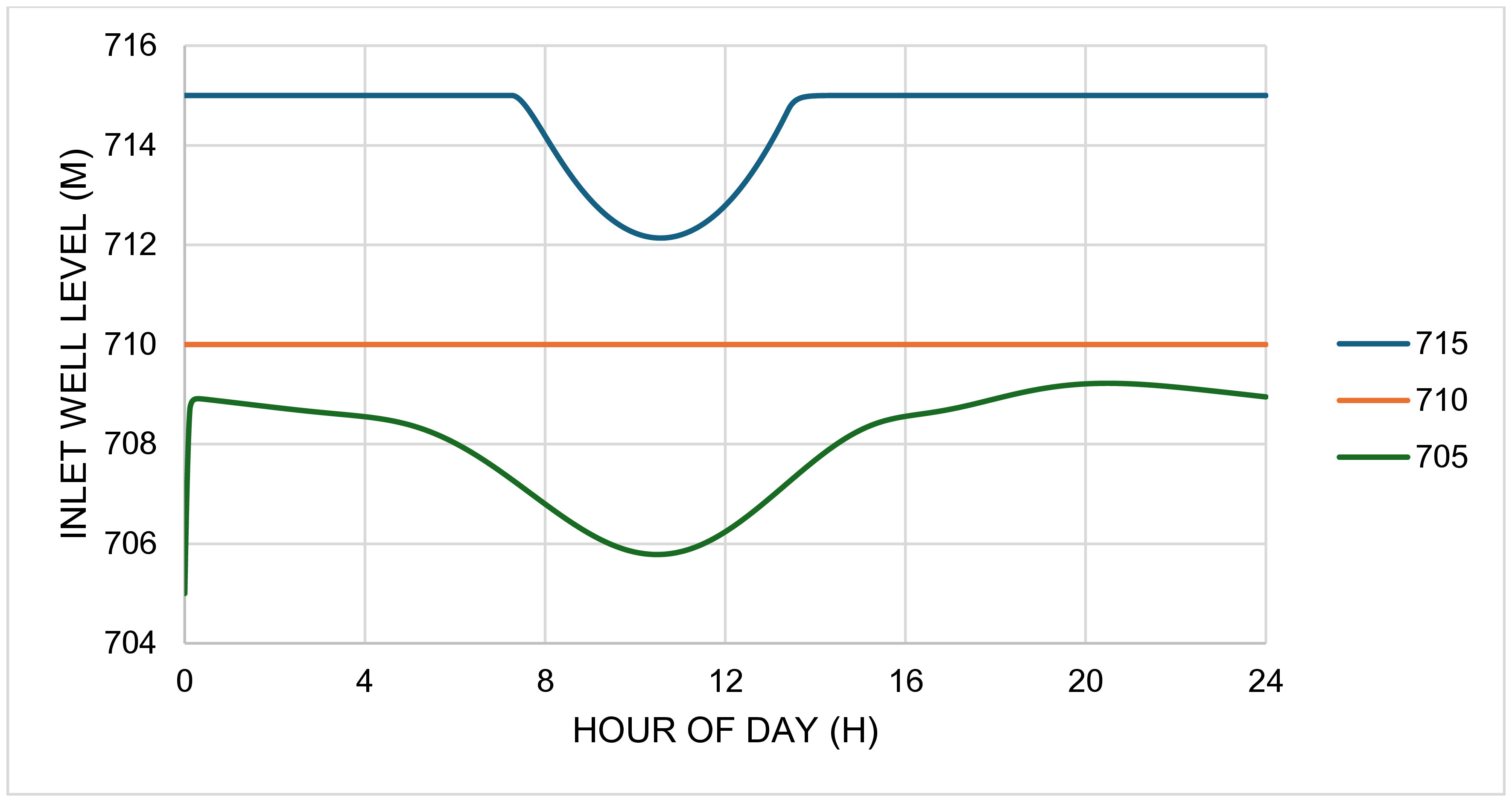
The results presented in this section correspond to the simulation of three operational scenarios, defined by the reference levels $z_{ref}=705$, $710$ and $715m$, applied to the control of Systems 3 (variable-speed) and 4 (constant-speed). Based on the proposed methodology, the algorithm developed in this study was executed and, in what follows, the results obtained for the different simulated conditions are presented. It is also noted that, for the calculation of the target flow rate used by the controller, an abstract time step $\Delta t_{cor}=600s$ was adopted, employed exclusively as a mathematical control parameter, with no direct physical influence on the hydraulic system. Figure 8 shows the operation of the variable-speed pump over a 24-hour period, compared with the sewage discharge $Q_{ef}\left(t\right)$, evidencing the controller’s response for each reference level. Figure 9 displays the operation of the constant-speed pump, Figure 10 presents the evolution of the inlet well level $z_1\left(t\right)$ for the three simulated scenarios, while Figure 11 shows the rotational ratio $\alpha \left(t\right)$ applied to the variable-speed unit.

Figure 8
Variable-speed pump flow rate (m³/s) over the day for reference levels 705, 710 and 715 m, compared with the influent flow rate Qef​.

Figure 9
Constant-speed pump flow rate (m³/s) over the day for reference levels 705, 710 and 715 m, compared with the influent flow rate Qef.

Figure 10
Inlet well water level z1​ over the day for the three reference scenarios.

Figure 11
Speed ratio of the variable-speed pump for the three reference scenarios.

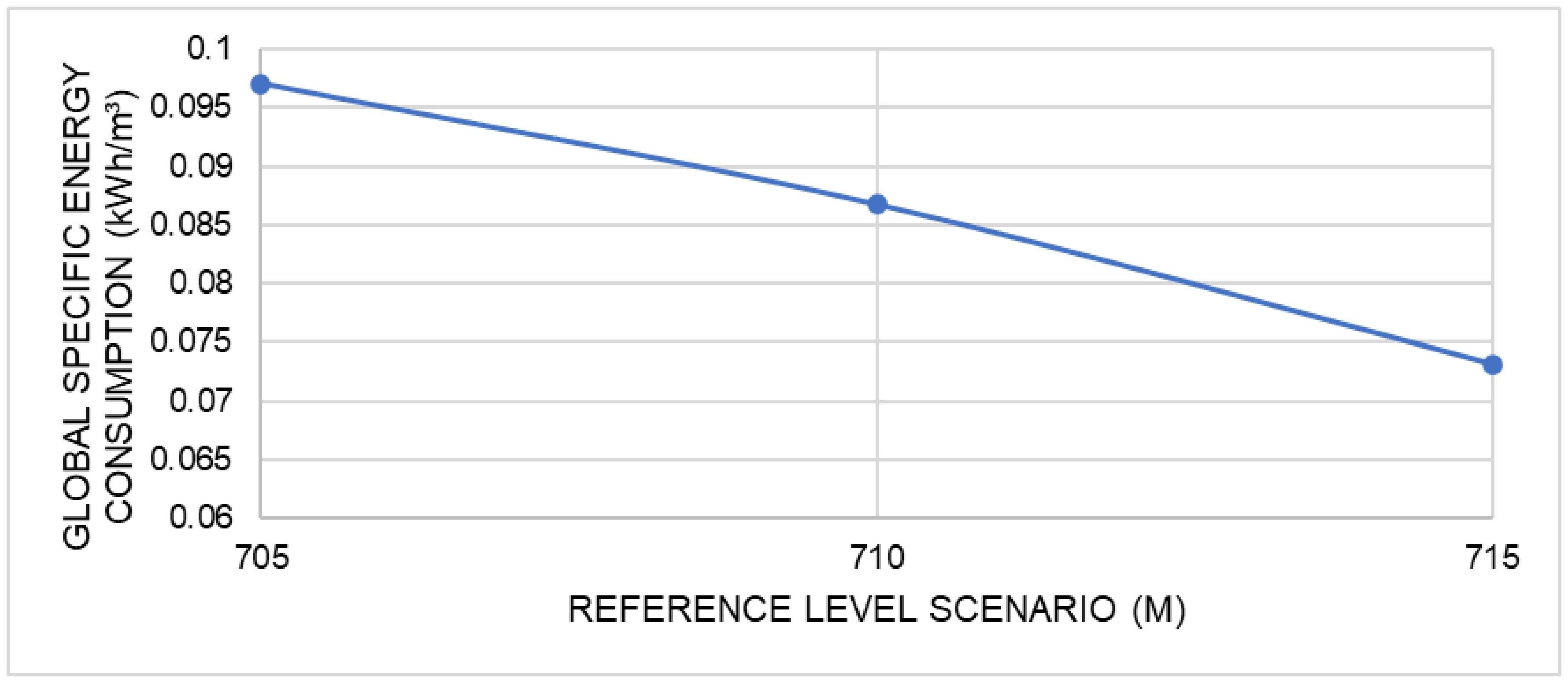
Figures 12and 13 illustrate the instantaneous specific energy consumption of the variable-speed and constant-speed pumps, respectively. Finally, Figure 14 consolidates the global daily energy index for each reference level $z_{ref}$, provided by Equation 18​.

Figure 12
Specific energy consumption (kWh/m³) of the variable-speed pump for the three reference scenarios.

Figure 13
Specific energy consumption of the constant-speed pump for the three reference scenarios.

Figure 14
Global specific energy consumption for the evaluated reference level scenarios.

A specific weight of $\gamma =9810N/m^3$ was adopted throughout the calculations. Although sewage presents slightly different physical properties, such differences do not produce relevant deviations in the resulting energy indicators. In the scenario with $z_{ref}=715m$, the inlet well level decreases between approximately 7.5 and 14 hours. This occurs because, during this interval, the pumping capacity exceeds the incoming sewage discharge, which reaches its lowest daily values in that period. Under this condition, the variable-speed pump remains continuously at the minimum rotational ratio $\alpha =0.75$ (Figure 10). Although the pump could be shut down, this action is avoided to prevent hydraulic transients and repeated start–stop cycles, which adversely affect efficiency and pump longevity. In the opposite scenario, at $z_{ref}=705m$, the variable-speed pump operates at $\alpha =1.00$ for almost the entire day, yet the level $z_1\left(t\right)$ does not reach the reference elevation.

This result demonstrates that, at this lower setpoint, the two operating pumps are not sufficient to compensate for the incoming flow, even with the variable-speed unit at nominal rotation. Although activating a third pump would hydraulically restore the level, such action would contradict the central purpose of this work, which is to pursue energy efficiency rather than simply meeting the hydraulic setpoint. Figures 12 and 13 show that the specific energy consumption of the variable-speed pump exhibits greater oscillation, a direct consequence of the continuous adjustments in rotational ratio throughout the day. In the scenario $z_{ref}=705m$, for instance, the instantaneous specific consumption reaches approximately 0.13kWh/m³ during the period of lowest sewage discharge, while the constant-speed pump, in the same interval, presents a value near 0.11kWh/m³. This contrast highlights the operational relevance of the constant-speed unit, which dampens the demand imposed on the variable-speed pump and contributes to stabilizing the hydraulic–energy behavior of the system. Indeed, the specific energy consumption of the constant-speed pump shows a more uniform trend. In the intermediate scenario, $z_{ref}=710m$, where $z_1\left(t\right)$ remains nearly constant, the constant-speed unit operates at approximately 0.087kWh/m³, whereas the variable-speed pump shows higher consumption in the central part of the day, when corrective actions are more intense. In all scenarios, the total pumped volume over the 24-hour period was approximately ${10}^6{m}^3$, with a variation of about ±3000m³ (roughly 0.3%). This result is consistent with the Fourier-based curve and with the integral of Equation 13, confirming both the volumetric balance and the hydraulic consistency of the numerical model.

It is important to emphasize that the reference level is not always reached, as it depends on the magnitude of the incoming discharge $Q_{ef}\left(t\right)$ relative to the pumping capacity. In the most critical situation, corresponding to $z_{ref}=705m$, the system is unable to overcome the inflow, and the level does not reach the setpoint, as shown in Figure 10. Conversely, in the opposite extreme, for $z_{ref}=715m$, both pumps exceed $Q_{ef}\left(t\right)$ during midday, causing the level to drop below the reference value, which is also clearly observed in Figure 10.

Despite the contributions presented, the study is subject to limitations that must be recognized. These limitations are primarily associated with the availability and quality of operational and design data. With respect to operational data, the relatively low temporal resolution of the measurements constrained the detailed characterization of short-term hydraulic and energetic dynamics, which may have attenuated transient responses relevant to pump performance and control actions. Regarding design data, uncertainties inherent to the available pump characteristic curves constitute an additional limitation, as these curves may not fully represent the actual in behavior of the equipment under variable operating conditions, progressive wear, or changing hydraulic environments. Accordingly, future investigations should incorporate higher-frequency monitoring and experimental recharacterization of pump curves to enhance the accuracy, robustness, and predictive capability of the proposed modeling framework.

CONCLUSIONS

The results demonstrate that the choice of the reference level $z_{ref}$​ has a direct influence on the energy performance of the pumping system. It was verified that selecting an appropriate operating level for the inlet well can lead to significant efficiency gains, reducing the specific energy consumption associated with the pump flow rates. As shown in Figure 14, the global specific energy consumption decreases from 0.097kWh/m³ in the scenario with $z_{ref}=705m$ to 0.073 kWh/m³ when $z_{ref}=715m$. In absolute terms, this reduction represents an energy saving of approximately 24,000 kWh per day, which is highly relevant for large-scale systems operating continuously. The results also indicate that a comprehensive understanding of pressurized-pipe hydraulics is essential to achieving such improvements, since the interaction among available head, distributed and local head losses, system head curve, and pump head curve directly defines the hydraulic operating point. Identifying operating zones with reduced dissipation allows the system to maximize energy efficiency during pumping. When combined with rotational control this knowledge translates into measurable operational benefits. The integration of design information (pump characteristic curves, reservoir geometry, and discharge elevation) with operational data (pump flow rate and inlet well level), together with Extended Period Simulation (EPS) and the application of mass and energy conservation equations, proved to be effective in representing the daily dynamics of the system and in quantifying the energy impact of different operating strategies. The consolidated metric $E_{global}$ showed consistent behavior and proved to be a robust indicator for comparing scenarios, enabling an objective evaluation of energy performance throughout the 24-hour cycle. It is therefore concluded that the careful definition of the operating level of the inlet well, combined with the use of variable-speed pumping, is an effective strategy for reducing energy consumption in wastewater pumping stations. In addition to lowering operational costs and improving energy efficiency, this approach contributes to the sustainability of the system and supports the expansion of sanitation services, aligning technical performance with the guidelines of the new Brazilian regulatory framework. Furthermore, the proposed model is generalizable and may be extended to other wastewater treatment plants and similar hydraulic systems, such as pressurized transmission mains, raw-water pumping stations, and distribution networks, in which pump control and level management directly affect overall performance.

This study’s main contributions are significant because they demonstrate, in a rigorous and quantitative manner, how the integration of real operational data, hydraulic modeling, and variable-speed pump control can effectively reduce energy consumption in large-scale wastewater systems without compromising hydraulic reliability. By linking theoretical hydraulics, numerical methods, project development and practical plant operation, the proposed approach provides a replicable framework for improving energy performance in pumping stations, supporting both economic efficiency and environmental sustainability in line with contemporary sanitation policies.

LIST OF ABBREVIATIONS AND SYMBOLS

BEP – Best Efficiency Point

CS – Constant-Speed

EPS – Extended Period Simulation

IW – Inlet Well

NF – number of fittings

NP – number of pipes

SNIS – Sistema Nacional de Informações sobre o Saneamento (Brazilian National Sanitation Information System)

VS – Variable-Speed

WWTP – Wastewater Treatment Plant

$a_0;a_n;b_n$ – harmonic coefficients (m³/s)

$A_H;B_H;C_H;D_H;E_H$ – head pump regression coefficients ($m;s{m}^{-2};s^2{m}^{-5};$

$s^3{m}^{-8};s^4{m}^{-11},$ respectively)

$A_R;B_R;C_R$ – resistance regression coefficients ($s^2{m}^{-5};s^3{m}^{-8};s^4{m}^{-11}$, respectively)

$A_{\eta };B_{\eta };C_{\eta };D_{\eta };E_{\eta }$ – efficiency pump regression coefficients (non-dimensional; $s{m}^{-3}$; $s^2{m}^{-6};s^3{m}^{-9};s^4{m}^{-12}$, respectively)

$A$ – internal cross-sectional pipe area (m²)

$A^{*}$ – upstream cross-sectional pipe area (m²)

$D$ – internal pipe diameter (meters)

$E$ – specific energy consumption (kWh/m³)

$E_{global}$ – global specific energy consumption (kWh/m³)

$f$ – friction factor (non-dimensional)

$g$ – gravitational acceleration (m/s²)

$H$ – head

$H_B$ – pump head (meters)

$\Delta H$ – static head (meters)

$k$ – minor loss coefficient (non-dimensional)

$L$ – pipe length (meters)

$n$ – harmonic order

$Q$– flow rate (m³/s)

$Q_B$ – pumped flow rate (m³/s)

$Q_{CS}$ – constant speed pump flow rate (m³/s)

$Q_{ef}$ – effluent discharge (m³/s)

$Q_n;Q_{n+1}$ – iterative flow rate steps

$Q_{target}$ – target flow rate (m³/s)

$Q_{VS}$ – variable speed pump flow rate (m³/s)

$R$ – hydraulic resistance ($s^2{m}^{-5}$)

$R²$ – coefficient of determination (non-dimensional)

$t$ – time (seconds)

$\Delta t$ – time interval (seconds)

$\Delta t_{cor}$ – correction time interval (seconds)

$T$ – period (seconds)

$z_1;z_2$ – upstream and downstream water level, respectively (meters)

$\alpha$ – rotational speed ratio (non-dimensional)

$\gamma$ – specific weight of the fluid (N/m³)

$\eta$ – pump efficiency (non-dimensional)

${\forall }_{cor}$ – volume correction (m³)

DATA AVAILABILTY STATEMENT

Research data is available in the body of the article.

ACKNOWLEDGEMENTS

The authors would like to acknowledge SABESP (Companhia de Saneamento Básico do Estado de São Paulo) for permitting technical visits, which were essential for a better understanding of the system. The authors also express their gratitude to Bruno Oliveira Nascimento for providing access to the database used in his research, which was developed under a partnership project between SABESP/FDTE-EPUSP.

REFERENCES

• Brasil. (2020, 15 de julho). Lei nº 14.026, de 15 de julho de 2020. Altera a Lei nº 9.984, de 17 de julho de 2000, e atualiza o Marco Legal do Saneamento Básico. Diário Oficial [da] República Federativa do Brasil, Brasília.
• Chapra, S. C., & Canale, R. P. (2011). Métodos numéricos para engenharia (5. ed.). McGraw-Hill.
• Gülich, J. F. (2003). Effect of Reynolds number and surface roughness on the efficiency of centrifugal pumps. Journal of Fluids Engineering, 125(4), 670-679. https://doi.org/10.1115/1.1593711
  » https://doi.org/10.1115/1.1593711
• Idelchik, I. E. (2007). Handbook of hydraulic resistance (4th ed.). Begell House.
• Mays, L. W. (2000). Water distribution systems handbook McGraw-Hill.
• Móller, D. S., Lima, G. M., Brentan, B. M., & Barros, D. B. (2020). Optimal pump selection for variable speed operation in water distribution network. Revista Brasileira de Recursos Hídricos, 25, e49. https://doi.org/10.1590/2318-0331.252020190093
  » https://doi.org/10.1590/2318-0331.252020190093
• Nascimento, B. O. (2024). Análise hidráulica de sistema elevatório final e de tanques de aeração de estação de tratamento de esgoto por lodo ativado com foco em eficiência energética – Estudo de caso ETE Barueri (Dissertação de mestrado). Escola Politécnica, Universidade de São Paulo, São Paulo.
• Noyola, A., Padilla Rivera, A., Morgan Sagastume, J. M., Güereca, L. P., & Hernández Padilla, F. (2012). Typology of municipal wastewater treatment technologies in Latin America. Clean (Weinheim), 40(9), 926-932. https://doi.org/10.1002/clen.201100707
  » https://doi.org/10.1002/clen.201100707
• Panepinto, D., Fiore, S., Zappone, M., Genon, G., & Meucci, L. (2016). Evaluation of the energy efficiency of a large wastewater treatment plant in Italy. Applied Energy, 161, 404-411. https://doi.org/10.1016/j.apenergy.2015.10.027
  » https://doi.org/10.1016/j.apenergy.2015.10.027
• Porto, R. M. (2006). Hidráulica básica (4. ed.). EESC-USP.
• Sistema Nacional de Informações sobre o Saneamento – SNIS. (2025, 23 de janeiro). Retrieved in 2025, January 23, from https://www.gov.br/cidades/pt-br/acesso-a-informacao/acoes-e-programas/saneamento/snis
  » https://www.gov.br/cidades/pt-br/acesso-a-informacao/acoes-e-programas/saneamento/snis
• Tullis, J. P. (1989). Hydraulics of pipelines: pumps, valves, cavitation, transients Hoboken: John Wiley & Sons. https://doi.org/10.1002/9780470172803
  » https://doi.org/10.1002/9780470172803
• Walski, T. M., Chase, D. V., & Savic, D. A. (2001). Water distribution modeling Waterbury: Haestad Press.
• Water Environment Federation. (2002). Activated sludge (Manual of Practice OM-9, 2nd ed.). Water Environment Federation.
• White, F. M. (2011). Mecânica dos fluidos (6. ed.). McGraw-Hill.

Edited by

• Editor in-Chief:
  Adilson Pinheiro

• Associated Editor:
  Iran Eduardo Lima Neto

Publication Dates

• Publication in this collection
  10 July 2026
• Date of issue
  2026

History

• Received
  28 Oct 2025
• Reviewed
  22 Mar 2026
• Accepted
  25 Mar 2026