Large Eddy Simulations of extreme pressures in low Froude number hydraulic jumps

Simulações de Grandes Escalas de pressões extremas em ressaltos hidráulicos com baixos números de Froude

Abstract

This paper sought to assess the capability of the Large Eddy Simulation technique in reproducing the fluctuating pressures exerted on the slabs of hydraulic jump stilling basins. Using the volume-of-fluid (VOF) technique and the Smagorinsky model, three hydraulic conditions were simulated, with inflow Froude numbers equal to 2.3, 3.0 and 3.8. After grid verification, the simulations were validated through the comparison of extreme pressure quantiles and mean and standard deviation of velocities. Instantaneous pressure series extracted from the numerical simulations were compared against data from other experimental works, comprising the pressure fluctuations coefficient and dimensionless quantiles of extreme pressures. The Large-Eddy Simulation (LES) technique was found to be able to generate instantaneous pressure series of low Froude number jumps with adequate probability distributions. Intensity of pressure fluctuations and extreme pressure values acting on low Froude number stilling basins can be readily computed using the equations proposed herein.

Keywords:
Extreme pressures; Pressure fluctuations; Low Froude number hydraulic jumps; Stilling basins; Large Eddy Simulation

Resumo

Este artigo buscou avaliar a capacidade da técnica de Simulação de Grandes Escalas em reproduzir as pressões flutuantes exercidas sobre as lajes de bacias de dissipação por ressalto hidráulico. Empregando a técnica volume-de-fluido (VOF) e o modelo de Smagorinsky, três condições hidráulicas foram simuladas, com números de Froude incidentes iguais a 2.3, 3.0 e 3.8. Após verificação das malhas, as simulações foram validadas por meio da comparação de quantis de pressões extremas e da média e dos desvios-padrão das velocidades. Séries de pressões instantâneas extraídas das simulações numéricas foram comparadas com outros estudos experimentais, abrangendo os coeficientes de flutuação de pressão e quantis adimensionais de pressões extremas. Verificou-se que a técnica de Simulação de Grandes Escalas (LES) é capaz de gerar séries de pressões instantâneas de ressaltos hidráulicos com baixos números de Froude com distribuições de probabilidade adequadas. A intensidade de flutuações de pressão e valores extremos de pressão atuando em bacias de dissipação com baixos números de Froude podem ser prontamente calculadas empregando as equações aqui propostas.

Palavras-chave:
Pressões extremas; Flutuações de pressão; Ressaltos hidráulicos com baixos números de Froude; Bacias de dissipação; Simulação de Grandes Escalas

INTRODUCTION

Despite the combined effort of numerous researchers, since when the hydraulic jump was first described and sketched by Leonardo da Vinci at the turn of the 15^th to the 16^th century (De Padova & Mossa, 2021), there are still research gaps regarding this phenomenon. Unlike classic stable jumps, which have already been extensively studied, low Froude number jumps still need advancements regarding their bottom pressure and velocity fields, as they have received less attention from the perspective of hydraulic engineering applications.

The Froude number $\text{F}=v/{\left(gy\right)}^{0.5}$ (in which $v$ and $y$ are, respectively, the depth-averaged velocity and the hydraulic depth, while $g$ is the gravitational acceleration) is a dimensionless quantity expressing the ratio between inertial and gravitational forces of an open channel flow. Conventionally, when computed at the inflow section of the hydraulic jump, subscript 1 is used. According to the classification presented by Chow (1959) and Elevatorski (1959), a hydraulic jump is said to have a low Froude number if 1.7 <${\text{F}}_1$< 4.5. Despite its lower energy dissipation when compared to a stable jump (4.5 <${\text{F}}_1$< 9.0), a low Froude number jump might be chosen as the design condition of the energy dissipator of a dam, depending on the hydraulic and topographic conditions of the project.

The occurrence of low Froude number hydraulic jumps at the dam toe is favored by factors such as a low-sloped river with high discharges, which is exactly the case for most of the hydropower plants built in the Amazon region (slopes of Amazon rivers are of the order of 0.003% and, according to Richey et al. (1989), the mean annual discharge at the mouth of the Amazon River is 200,000 m³/s). Furthermore, the Northern region has the greatest available hydropower potential of Brazil: 43% of the country’s total estimated hydropower potential of 261.4 GW (Brasil, 2007).

With the diffusion of instruments such as pressure transducers, Prandtl-Pitot tubes and hot-wire anemometers, the period between the 1960s and the 1990s saw many studies characterizing pressure and velocity fields of jumps, mostly stable ones. Worth mentioning are the works of Vasiliev & Bukreyev (1967), King (1967), Abdul Khader & Elango (1974), Toso & Bowers (1988) and Fiorotto & Rinaldo (1992), whose studies comprised the analysis of several statistical metrics computed with the instantaneous pressures transmitted by the jump to the stilling basin. From the 2000s, applications of computational fluid dynamics on the hydraulic jump case became prominent. Some examples are the works of Amorim et al. (2004), Gonzalez & Bombardelli (2005), Carvalho et al. (2008), Ma et al. (2011) and Valero et al. (2014). Due to the advantages and limitations of each approach (physical and computational), the current scenario acknowledges that they complement each other. The emergence of eddy-solving techniques, such as DNS (Direct Numerical Simulation) and LES (Large Eddy Simulation), proved that Computational Fluid Dynamics (CFD) is capable of yielding turbulent quantities of the flow, even in the smallest scales. The current limitation to that, though, is the elevated computational costs required, often not feasible for engineering practical applications.

Regarding the extraction of pressures in hydraulic jumps through CFD, few studies can be found in literature. Amorim et al. (2004), Carvalho et al. (2008), Macián-Pérez et al. (2020) and more recently Santos et al. (2022) and Bocchi et al. (2024) analyzed pressures obtained through RANS (Reynolds-Averaged Navier Stokes equations) based simulations. All of them achieved good results when compared to experimental data of mean pressures along the jump. Although Macián-Pérez et al. (2020) also compared numerical and experimental values of pressure fluctuations, no good agreement was found between the two approaches. The pressure fluctuations obtained by Jesudhas et al. (2018), using a DES (Detached Eddy Simulation) model of a hydraulic jump with ${\text{F}}_1$= 8.5, showed good agreement with experimental data. However, this comparison was merely used for validation purposes, and no deeper analysis was performed with the data. Mortazavi et al. (2016) performed a DNS of a jump with ${\text{F}}_1$= 2, but their analysis concerning pressures comprised only mean values. A good agreement between experimental and numerical values of mean, minimum and maximum pressures, as well as pressure fluctuations, was obtained by Lu et al. (2021), who used the LES model of FLOW-3D® to carry out simulations of hydraulic jumps (4.2 <${\text{F}}_1$< 5.3) occurring on a stilling basin slab with a bottom drop and sudden lateral enlargement. Li et al. (2022) employed CFD to study pressure fluctuations, applying a DES model to an aerator negative step of a spillway tunnel. When compared with experimental data, the simulations yielded good results of pressure fluctuation coefficient $C_p^{\text{'}}$ and probability density of pressures. No design equations for extreme pressures in hydraulic jumps have been provided by the aforementioned studies based on eddy-resolving techniques (DNS, LES or DES).

Thus, to the extent of the authors’ knowledge, there are currently no CFD studies extensively focusing on the analysis of extreme and fluctuating pressures in low Froude number hydraulic jumps nor any study mentioning the computational effort (or the grid refinement) needed for obtaining such pressures. A lack of equations for the estimation of these metrics was also identified. Considering the small, medium and especially the two large hydropower plants (HPPs) planned for the Amazon region (Tabajara HPP and Bem Querer HPP, adding up to 1.05 GW) for the next decade alone (Brasil, 2022), and aiming to fill the previously mentioned literature gaps, the present study analyses instantaneous pressure series extracted from large-eddy simulations of three flow conditions of low Froude number hydraulic jumps carried out with the Smagorinsky turbulence model. A comparison with previously published experimental data is also included, together with the proposal of equations for the estimation of pressure fluctuations and extreme pressures throughout the jump.

MATERIALS AND METHODS

Experimental data

The simulations presented here were based on three experiments of low Froude number hydraulic jump carried out by Steinke Júnior (2020), with unit flow rates $q$ equal to 0.0625 m²/s, 0.125 m²/s and 0.250 m²/s. These hydraulic conditions (Cases I, II and III, respectively) correspond to incident Froude numbers ${\text{F}}_1$ equal to 3.8, 3.0 and 2.3, and inflow depths $y_1$ equal to 0.030 m, 0.057 m and 0.108 m. Steinke Júnior et al. (2021) statistically analyzed the instantaneous pressures of these jumps, measured at the centerline of the flume with pressure transducers. These pressure data are used in the present paper as a benchmark for the instantaneous pressures extracted from the numerical simulations, as well as data presented by Toso & Bowers (1988), Endres (1990), Dai Prá (2011) and Hampe (2018).

New experiments were carried out on the same flume used by Steinke Júnior (2020), under the same hydraulic conditions (unit flow rate and downstream control) of Cases II and III, aiming to measure velocities to validate the numerical simulations. The velocities were point-wise measured at the central plane of the flume, with a downward-looking Sontek 16 MHz micro-Acoustic Doppler Velocimeter (ADV) during a period of 90 s at a rate of 50 Hz. Raw data were filtered through the phase-space threshold filter introduced by Goring & Nikora (2002). It was not possible to perform velocity measurements of Case I, since the hydraulic jump had low water depths and mostly a highly aerated flow, which prevented the ADV from properly measuring velocities in the roller region. This was also the case for the upstream portion of the hydraulic jump of Case II and for the near-surface region. According to the manufacturer (SonTek/YSI, 2001), good results can be obtained for Signal-to-Noise Ratios (SNR) higher than 10 dB and correlations higher than 30% ‑ 40%, which is the case for all ADV measurements presented herein.

Flow equations and turbulence treatment of numerical simulations

The interface FLOW-3D HYDRO® (Version 22.1, Flow Science Inc., 2022) was used to run the simulations. The software solves the Navier-Stokes equations using the finite volume method (McDonald, 1971) and the VOF (volume of fluid) scheme (Hirt & Nichols, 1981). Standard time discretization and CFL-based time stepping were applied (Flow Science Inc., 2023), with maximum CFL number set to 0.45.

Although the Smagorinsky model is known to induce overestimated dissipation, it is currently the only available option for running LES in FLOW-3D and was, therefore, used in the main simulations. The main simulations (the ones performed with the LES technique) were carried out using the Smagorinsky model. According to this model (Smagorinsky, 1963), after filtering the incompressible Navier-Stokes equations, a sub-grid scale stress ${\tau }_{ij}$ is introduced in the momentum equation, which is computed as

${\tau }_{ij}-\frac{{\tau }_{kk}{\delta }_{ij}}{3}=-2{\nu }_t\overline{S_{ij}}$ (1)

with ${\delta }_{ij}=\left\{\begin{array}{c}\mathrm{0,}i\ne j\\ \mathrm{1,}i=j\end{array}\right.$ and the strain rate tensor $\overline{S_{ij}}=\frac{1}{2}\left(\frac{\partial \overline{u_i}}{\partial x_j}+\frac{\partial \overline{u_j}}{\partial x_i}\right)$. The turbulent viscosity ${\nu }_t$ is then computed according to ${\nu }_t={\left(C_s\Delta \right)}^2\sqrt{2\overline{S_{ij}}\overline{S_{ij}}}$, in which $C_s$ is the Smagorinsky coefficient, that was assumed as being 0.1 in this study, as in Li et al. (2018). Furthermore, three simulations were carried out using the RNG $k$-ε turbulence model, a RANS-based approach proposed by Yakhot et al. (1992). The goal of these simulations was to generate a rough estimate of the turbulence length scales occurring in the hydraulic jumps here studied.

Simulation settings

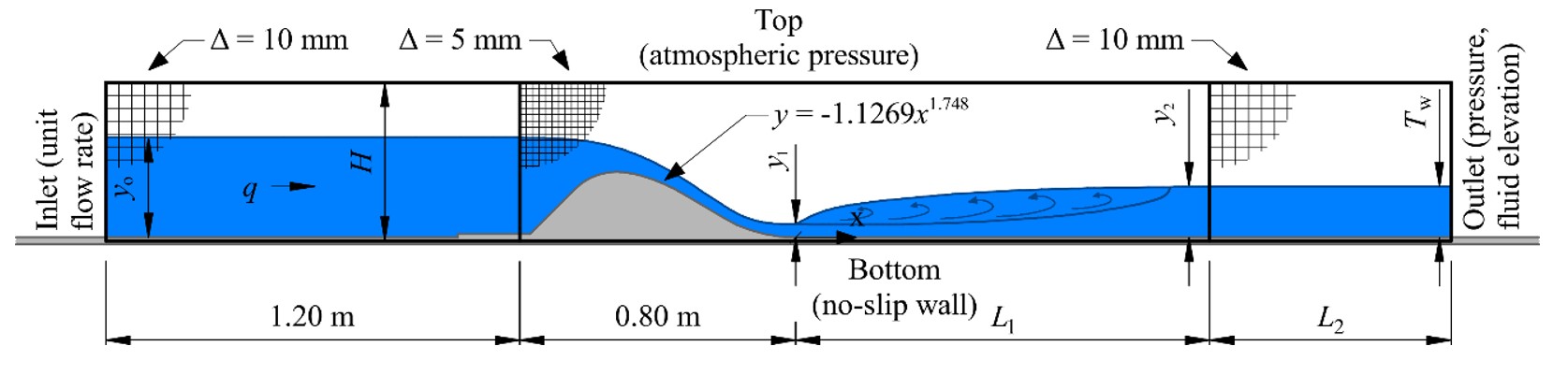
Figure 1 is a longitudinal cross section of the geometry configuration used, based on the flume used by Steinke Júnior (2020). Several studies on the hydraulic jump analyze its occurrence downstream of a sluice gate (Ghaderi et al., 2020; Jesudhas et al., 2018; Liu et al., 2004), or far away from any upstream or downstream controls (Macián-Pérez et al., 2020; Mortazavi et al., 2016). Here, however, the hydraulic jump is analyzed occurring downstream of a spillway, in a stilling basin, similarly to Amorim et al. (2015), Valero et al. (2018) and Lu et al. (2021). Therefore, the simulation domain was configured to comprise the spillway as well, so that its effects on the jump were considered. The motivation behind this was the differences observed between jumps downstream of sluice gates and those downstream of spillways, mainly because of the toe curve effects on the pressures at the beginning of the stilling basin (Dai Prá, 2011; Toso & Bowers, 1988).

Figure 1
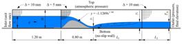
Sketch of numerical simulation settings: geometry (spillway in grey), boundary conditions, chosen grid, relevant variables and example of “stabilized” state (water phase in blue, air phase in white).

Table 1 presents information on each test case. Coordinates $x$ and $y$ correspond to the longitudinal and vertical axes, respectively. The origin of the coordinate system is at the junction between the spillway toe and the stilling basin, such that the coordinate $x$= 0 m corresponds to the upstream end of the basin. The test flume is 40 cm wide, both in the experimental model and in the numerical simulations. The variables $H$, $L_1$ and $L_2$, which are used to assemble the total length and height of the numerical domain (Figure 1), vary for each test case and assume the values presented in Table 1.

Table 1
Geometric and boundary conditions and information on the jumps tested.

Case	$q$ (m2/s)	$y_o$ (m)	$H$ (m)	$L_1$ (m)	$L_2$ (m)	$T_w$ (m)	$y_1$ (m)	$F_1$
I	0.0625	0.300	0.35	1.20	2.00	0.1500	0.030	3.8
II	0.1250	0.341	0.40	1.50	2.30	0.2140	0.057	3.0
III	0.2500	0.416	0.46	1.80	2.20	0.3035	0.108	2.3

For each test case, a structured hexahedral mesh was configured, made up of three regions (Figure 1). The main region comprised the spillway and the greater part of the stilling basin, for which cubic cells with side $\text{Δ}$= 5 mm were specified (in the finally chosen mesh). The regions upstream of the spillway and downstream of the jump, of lesser interest, were represented by cells of $\text{Δ}$= 10 mm. The grid choice process, which comprised two other coarser grids, is detailed further ahead.

The boundary conditions of the numerical scheme are shown in Figure 1. For the lateral and bottom walls and for the spillway, the no-slip condition (i.e., zero velocity relative to the boundary) was specified, as well as a roughness height of 0.05 mm to represent the plexiglass. The top plane boundary condition was the atmospheric pressure. Constant volumetric unit flow rates $q$ were specified for the upstream most section, associated with the upstream flow depths $y_o$ experimentally measured by Steinke Júnior (2020), according to Table 1. As for the downstream boundary condition, the tailwater depth $T_w$ was manually adjusted until the jump occurred at the desired position (time-average of oscillating jump toe at $x$ = 0 m). Table 1 contains the final values of $T_w$ used as the downstream boundary condition.

The simulations were considered to have converged when the volume of fluid inside the domain stabilized. From this stabilized state (example shown in Figure 1), another 30 s were simulated, from which the instantaneous pressure data were extracted. This was performed with the aid of probes created on the flume bottom along its longitudinal axis, writing data at a sampling frequency of 400 Hz. The clock time needed to process 30 s of simulation using the chosen grid, in a machine with 8 cores @ 3.80 GHz and 64 GB of RAM memory, was 56, 94 and 123 hours respectively for Cases I, II and III. The time-step for the simulations run with the final grid was, on average, equal to 1.8×10^-4s.

According to the Flow-3D® User’s Manual (Flow Science Inc., 2023), in order to estimate the air entrainment rates, FLOW-3D® considers the balance between the stabilizing forces (surface tension and gravity) and destabilizing forces (turbulent kinetic energy). Although aeration is an important feature of the hydraulic jump, air entrainment is known to be less pronounced in low Froude number jumps, when compared to higher values (Rajaratnam, 1967; Gualtieri & Chanson, 2007). In the type of jump analyzed here, the two-phase flow is mainly confined to the roller region, while the oscillating jet beneath it remains weakly aerated. Since aeration was not the focus of this study, a first order approximation that reproduces the effects of the density non-uniformity resultant from air entrainment was considered sufficient for the present purposes.

Grid choice

Three grids were tested for the simulations here presented. Table 2 contains the element size of each grid and the total cell count $N_{cells}$ within the simulation domain for each Case. The side of the cubic cells in the upstream and downstream region was always two times that of the cells in the main region.

Table 2
Information on grids tested.

Grid	Element size (main region)	Total cell count ($N_{cells}$× 106)
		Case I	Case II	Case III
A	$\Delta$= 5 mm	2.69	3.50	4.45
B	$\Delta$= 7 mm	1.00	1.32	1.63
C	$\Delta$= 10 mm	0.34	0.44	0.56

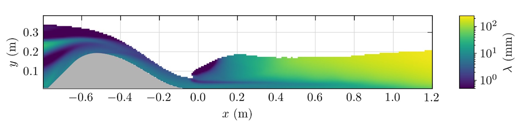
For a first rough estimate of the level of refinement needed for the large-eddy simulations, three simulations (one for each Case) were carried out using the RNG k-ε turbulence model, employing Grid B. The results of turbulent length scale $\lambda$ (computed as $\lambda =k^{3/2}/\epsilon$) at the central plane of the flume for Case II (${\text{F}}_1$= 3.0), averaged over 30 seconds, are shown in Figure 2. Cases I and III presented similar behaviors and were, therefore, omitted here for brevity. Conceptually, at least 2 elements in each direction are needed to resolve a simple eddy. From that assumption, Grid A would be capable of representing primitive eddies with a minimum length scale of 10 mm (two times the element size $\Delta$). For Cases I, II and III, the number of cells within the central plane of the stilling basin, with a turbulent length scale higher than 0.01 m, was 64.6%, 81.0% and 78.6%.

Figure 2
Time-averaged turbulent length scales $\lambda$ for Case II, computed from RNG k-ε results.

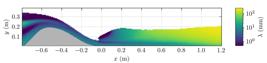
It is clear from Figure 2 that most characteristic eddies inside the stilling basin are well represented by Grid A ($\lambda$> 10 mm), especially for the region defined by $x$> 0.2 m. A good representation of these eddies is relevant for the purposes here intended, since, according to Li et al. (2022), the pressure fluctuation characteristics are primarily controlled by large-scale coherent eddies.

The Index of Resolution Quality for Large Eddy Simulations ($I{Q}_{LES}$) proposed by Celik et al. (2005) was employed to assess the quality of the mesh used in the main simulations. This performance index is based on the Richardson Extrapolation concept and can be applied to compare an LES with either a DNS, a physical experiment or even another LES that was run with a different mesh. For this last situation (comparison between 2 large eddy simulations with different grids), $I{Q}_{LES}$ is computed by

$I{Q}_{LES}=\frac{1}{1+\left(1-\frac{k_{res,c}}{k_{res,f}}\right){\left({\beta }^m-1\right)}^{-1}}$ (2)

in which $k_{res,f}$ and $k_{res,c}$ are respectively the resolved turbulent kinetic energies of the finer and coarser grids being analyzed, $\beta ={\Delta }_c/{\Delta }_f$ is the ratio between the characteristic cell sizes of each grid and $m$ is the order of accuracy of the numerical scheme. According to Celik et al. (2005), a grid can be considered adequate for an LES when $I{Q}_{LES}$> 75%.

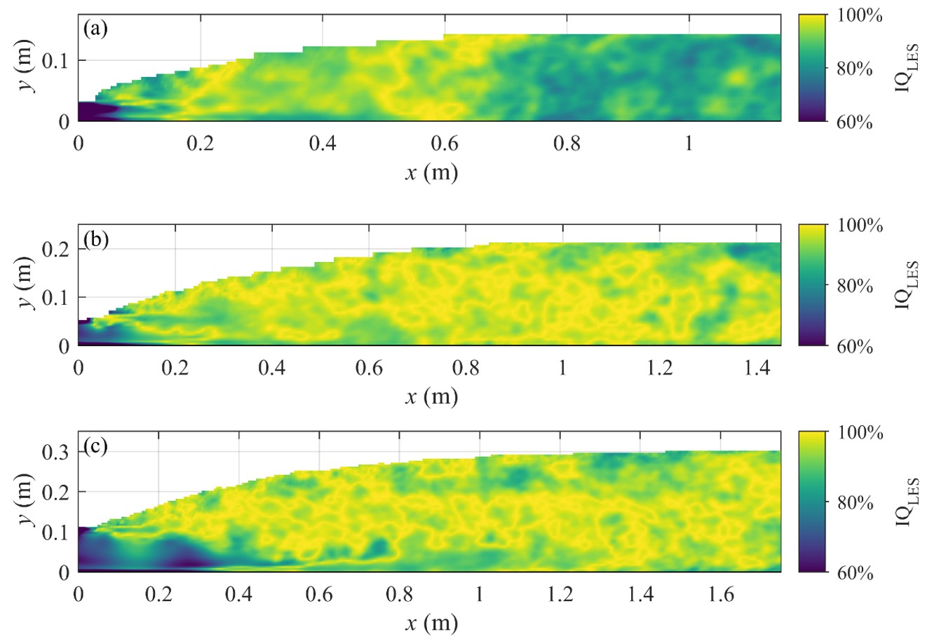
Figure 3 contains the $I{Q}_{LES}$ computed between grids A and C (for which $\beta$= 2) for 30 seconds of simulation, at the central plane of the flume. Except for the impinging jet region and some points in the downstream region of Case I, most of the quality indexes lie within the recommended range. The relatively short 30 s processing period may not have been sufficient to achieve statistical convergence of the $I{Q}_{LES}$ values, since the hydraulic jump is characterized by large-scale, low-frequency instabilities whose time scales exceed those of small-scale turbulence. Consequently, some localized discrepancies in $I{Q}_{LES}$ may result from the different instantaneous phases (“time windows”) of the hydraulic jump captured by the two grids analyzed. A longer averaging period would likely reduce these differences, although the overall predominance of $I{Q}_{LES}$ values above 75% still confirms that the flow was adequately resolved across most of the domain.

Figure 3
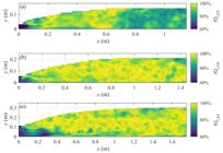
LES Index of Resolution Quality for the three flow conditions analyzed, computed between grids A and C: (a) Case I; (b) Case II; (c) Case III. Optimal range: $I{Q}_{LES}$> 75%.

Table 3 contains the ratios of cells of Grid A within the recommended range of $I{Q}_{LES}$, for each case and for values of $I{Q}_{LES}$ computed between Grids A and B, as well as the ones computed between grids A and C. Both pairings indicate a good resolution of Grid A, with the combination between Grids A and C yielding slightly better indexes. This is because more kinetic energy was resolved by Grid B, with respect to Grid C, and this is directly reflected in Equation 2. Considering that most cells inside the stilling basin fell within the optimal range, especially in the roller region and for the most part of the jump’s body, the resolution of Grid A was considered adequate for the purposes here intended.

Table 3
Percentage of cells of Grid A within the recommended range ($I{Q}_{LES}$> 75%).

Case	Grids A and B	Grids A and C
I	88.5%	98.4%
II	96.7%	98.8%
III	92.4%	96.7%

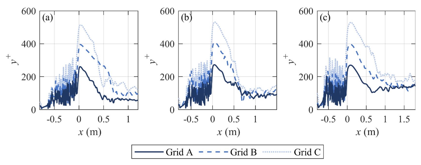
The dimensionless wall distance $y^{+}$ is computed as the product between the friction velocity at the nearest wall and the distance to that wall, divided by the fluid’s kinematic viscosity (Nieuwstadt et al., 2016). In the context of CFD, this parameter indicates the position of each cell’s centroid relative to the turbulent boundary layer. The analysis of wall-adjacent flow was limited to the centerline of the flume bottom (including the spillway and the stilling basin), where the instantaneous pressures were extracted. The values of dimensionless wall distance $y^{+}$ were plotted along the flume for each grid and are shown in Figure 4 for Cases I, II and III. Grids B and C yielded dimensionless wall distances of almost 400 and 600, respectively and therefore were deemed unsuitable, as they lie outside the range in which logarithmic law of the wall is typically valid (30 <$y^{+}$< 200~300). Meanwhile, Grid A produced considerably lower results than the others both in the spillway region ($x$< 0 m), and in the stilling basin ($x$> 0 m). Values of $y^{+}$< 200 were found almost everywhere for Grid A, except for a short stretch at the entrance of the stilling basin. Although these values do not indicate a fully-resolved near-wall turbulence, they lie within the range of applicability of the logarithmic law, and were therefore deemed acceptable for the purposes here intended.

Figure 4
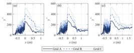
Values of dimensionless wall distance $y^{+}$ along longitudinal axis for each grid tested: (a) Case I; (b) Case II; (c) Case III.

Finally, Table 4 is a comparison between Grid A, used in the present study, and other works that used LES or DES to simulate the hydraulic jump: Jesudhas et al. (2017, 2018) and Lu et al. (2021). Both the characteristic cell size and the total cell count within the domain are of the same order of magnitude of the meshes used in the other studies. The ratio $y_1/\Delta$, which indicates how many cells, on average, are being used to represent the jump’s inflow section, also shows a good agreement with the literature used for comparison. From this comparison and the analyses performed above and considering that further refining the grid would result in impractical processing times, Grid A was chosen for the present study.

Table 4
Comparison with grids used in other LES-based studies on hydraulic jumps.

Work	$\overline{\Delta }$ (mm)	$N_{cells}$× 106	$F_1$	$R_1$	$y_1/\Delta$
Jesudhas et al. (2017)	~4.7	5.60	8.2	4.7×104	3.2
Jesudhas et al. (2018)	~3.5	7.00	8.5	7.8×104	5.7
Lu et al. (2021)	~20	~6.60	4.2 – 5.2	1.6 – 6.4×105	3.5 – 7.6
Present study	5	2.69	2.3	6.4×104	6.1
	5	3.50	3.0	1.3×105	11.4
	5	4.45	3.8	2.5×105	21.6

Validation

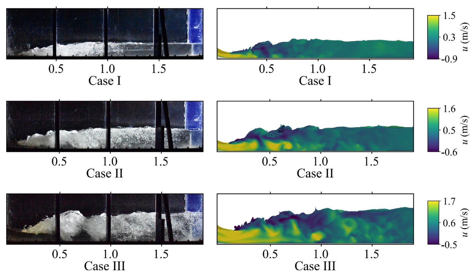
The comparisons presented herein aim at elucidating to what extent the numerical simulations are similar to the physical experiments. First, a visual and qualitative comparison is shown in Figure 5, which contains photographs of the physical hydraulic jumps from Steinke Júnior (2020) next to snapshots taken from the simulations, colored by the instantaneous longitudinal velocities $u$ occurring at the flume front wall. The side-by-side images reveal hydraulic jumps with similar dimensions, namely their overall lengths and depths, as well as the irregularities present on the free surface. The thickness and reach of the impinging jet, typical of low Froude number jumps (Steinke Júnior et al., 2021) are also well-represented by the numerical model.

Figure 5
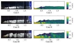
Visual comparison between physical (Steinke Júnior, 2020) and simulated hydraulic jumps (present study). Numerical results are colored by instantaneous longitudinal velocity $u$. Dimensions, in meters, are approximate due to perspective view.

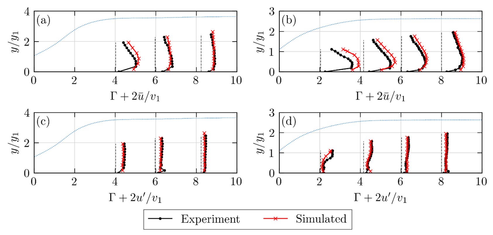
Figure 6 contains dimensionless profiles of longitudinal velocities extracted from the numerical simulations, in contrast with the velocities measured in the novel experiments, with the previously mentioned SonTek ADV. Both the experimental and the numerical data series were taken at the central plane of the flume. An approximation of the mean water surface is also presented. The velocity profiles, represented by the solid lines, were made dimensionless using the mean incident velocity $v_1$. Results are plotted with respect to the longitudinal positions where they were collected (dashed lines), made dimensionless through the difference between the sequent depths, $\Gamma$=$x$/($y_2$-$y_1$). The dimensionless velocity profiles were multiplied by a factor of 2 to ease visualization. The results of Figure 6 show good agreement of mean longitudinal velocities $\overline{u}$ and standard deviations of the longitudinal velocities $u^{\prime }$ computed by FLOW-3D and the ones measured experimentally.

Figure 6
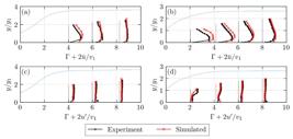
Dimensionless profiles of longitudinal velocities extracted from numerical simulations and collected with ADV: (a) Case II, mean; (b) Case III, mean; (c) Case II, standard deviation; (d) Case III, standard deviation.

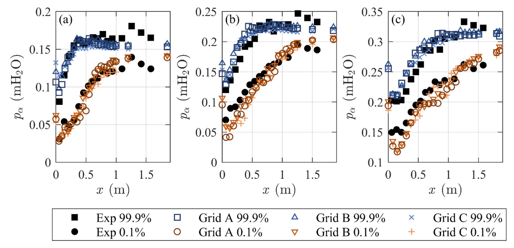
Dimensional extreme quantiles (percentages $\alpha$= 0.1% and $\alpha$= 99.9%) taken from the numerical series of instantaneous pressures occurring at the centerline of the flume are shown in Figure 7, in contrast with the experimental values collected by Steinke Júnior et al. (2021). Results from the three grids tested are shown and all compare well against the experimental data. The computational time required to run Grid A (56 h, 94 h and 173 h for Cases I, II and III, respectively) was significantly higher than to run Grid B (10.5 h, 18 h and 31 h). However, not much gain was noticed regarding the similarity of the numerical and the experimental data. This was the main reason for ceasing the grid refinement process, together with the rationale presented in the previous topic.

Figure 7
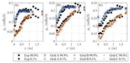
Numerical (present study) and experimental (Steinke Júnior et al., 2021) dimensional extreme pressures: (a) Case I; (b) Case II; (c) Case III. Differences observed between experimental and numerical data (from Grid A) correspond to less than 1 mH₂O error in prototype scale.

The Pearson correlation coefficients computed between the experimental and the numerical data (Grid A, interpolated at the correspondent longitudinal positions) resulted, for the three cases, in 0.967 <$r$< 0.988 for the minimum pressures ($\alpha$= 0.1%) and 0.916 <$r$< 0.950 for the maximum pressures ($\alpha$= 99.9%). These values were deemed acceptable, considering the uncertainties and sources of error that are intrinsic to both approaches. In terms of the mean absolute errors between the two series, Cases I, II and III resulted in errors of 0.0091, 0.0166 and 0.0172 mH₂O for $\alpha$= 0.1%, respectively, and errors of 0.0089, 0.0144 and 0.0172 mH₂O for $\alpha$= 99.9%. Considering the 1:50 scale of the physical model, these errors correspond to less than 1 mH₂O of pressure acting on the prototype structure.

RESULTS AND DISCUSSION

The study of fluctuating and extreme pressures is relevant due to a series of reasons. Firstly, pressure fluctuations constitute a manner of measuring the degree of turbulence occurring within hydraulic jumps (Abdul Khader & Elango, 1974) and can be linked to damages and even failures of hydraulic structures. Thus, these fluctuations should be taken into account in the design of energy dissipators, such as hydraulic jump stilling basins (Bowers & Toso, 1988). Furthermore, while maximum pressure fluctuations correspond to the maximum compressive loads to which the basin slabs will be subject, minimum pressures are relevant in the analysis of cavitation risk (Lopardo, 2002) and offer little resistance against the uplift forces that can occur under the basin linings.

The study of Steinke Júnior et al. (2021) revealed that, except for the region defined by $\Gamma$< 0.5, which is under the effect of the toe curve, the mean pressures of low Froude number hydraulic jumps behave similarly to those of stable jumps. Equations for the estimation of mean pressures already exist, such as the one introduced by Teixeira et al. (2004). Therefore, the results presented here will focus on the extreme and fluctuating pressures exerted by low Froude number hydraulic jumps to the stilling basin slabs.

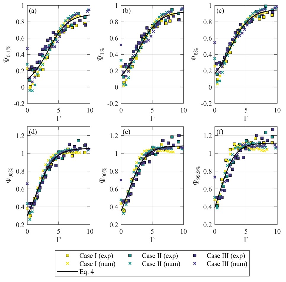
Dimensionless quantiles of extreme pressures for Cases I, II and III are shown in Figure 8, for minimum (probabilities $\alpha$= 0.1%, 1% and 5%) and maximum pressures (probabilities $\alpha$= 95%, 99% and 99.9%). The dimensional pressures $p_{\alpha }$, in equivalent head (mH₂O), were normalized as suggested by Marques et al. (1997):

Figure 8
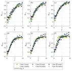
Dimensionless quantiles of extreme pressures and fitted curves: (a) $\alpha$= 0.1%; (b) $\alpha$= 1%; (c) $\alpha$= 5%; (d) $\alpha$= 95%; (e) $\alpha$= 99%; (f) $\alpha$= 99.9%. Number of events in sample $N$= 12,000.

${\Psi }_{\alpha }=\frac{p_{\alpha }-y_1}{y_2-y_1}$ (3)

The numerical data was taken from the simulations performed with Grid A. As previously shown in Figure 7, the numerical and the experimental data agree well with each other, despite the potential sources of error present in each approach. Thus, both datasets were used to fit curves that resulted in coefficients of determination of 0.899 <$r^2$< 0.949. All curves, each one for a different probability, can be described by Equation 4, together with the coefficients present in Table 5. It is noteworthy that the curves were derived from measurements performed on jumps occurring in a rectangular flume with Froude numbers ranging from 2.3 to 3.8 and are applicable only on jumps within this range.

Table 5
Input coefficients of Equation 4 and coefficient of determination ($r^2$) for different percentiles of pressure.

$\alpha$	$k_1$	$k_2$	$k_3$	$r^2$
0.1%	0.8961	8.1181	-0.6267	0.919
1%	0.9266	5.6852	-0.6089	0.933
5%	0.9519	4.8241	-0.6291	0.944
95%	1.0563	2.5133	-0.6898	0.949
99%	1.0844	2.0915	-0.7084	0.933
99.9%	1.1152	1.8477	-0.7972	0.899

${\Psi }_{\alpha }=\frac{k_1}{1+k_2.e^{k_3.\Gamma }}$ (4)

It is clear that, for more extreme values of $\alpha$, the data points are more scattered while, for milder values of $\alpha$, the points collapse better under one definite trend. Indeed, in a sample of 12,000 events (30 s × 400 Hz), the quantile $\alpha$= 95% corresponds to the 600^th highest value, while the quantile $\alpha$= 99.9% corresponds to the 12^th highest value, so the data is naturally expected to be more dispersed towards the ends of the probability distribution. Besides, the few mismatches observed between the datasets could also be due to slightly different positions of the jump (more upstream or downstream with respect to the spillway toe). Especially the region defined by $\Gamma$< 1.5 also presents a higher variability, which might be associated with the thickness of the impinging jet, as suggested by Steinke Júnior et al. (2021). This hints that a higher level of attention should be paid by the designer on this specific region when using the suggested curves.

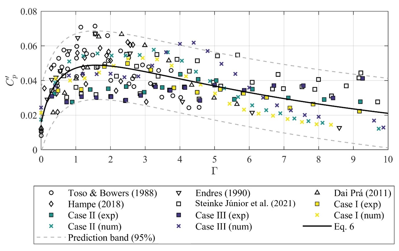
Figure 9 contains the pressure fluctuation coefficients $C_p^{\text{'}}$ computed for Cases I, II and III, in contrast with the respective experimental results from Steinke Júnior et al. (2021). The pressure fluctuation coefficients are computed from the standard deviations $\sigma$ of the series of instantaneous pressures, made dimensionless according to Abdul Khader & Elango (1974):

Figure 9
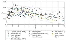
Pressure fluctuation coefficients of low Froude number hydraulic jumps: combination of original and literature data constitutes a comprehensive dataset for the range 1.7 <$F_1$< 4.5. Continuous line represents the overall $C_p^{\text{'}}$ trend, while dashed lines indicate the 95% prediction band.

$C_p^{\text{'}}=\frac{\sigma }{\left(v_1^2/2g\right)}$ (5)

Unlike extreme pressure quantiles, there was not such a strong agreement of pressure fluctuation coefficients between the results from the numerical simulations and the ones from the physical model. Firstly, it is known that pressure fluctuation coefficients of low Froude number jumps do not collapse together under a single definite trend with respect to the longitudinal position of the jump; rather, they scatter in a point cloud (Steinke Júnior et al., 2021). Furthermore, the coefficient $C_p^{\text{'}}$ is not only a function of the inflow Froude number, but, according to Toso & Bowers (1988), is also dependent on the degree of inflow development and on the measurement conditions, such as the duration of the test run and the chute slope. Besides, being a 2^nd-order statistical moment, it is evident that even the slightest perturbances and errors in the signal can be amplified such as to affect the results of the standard deviation. Finally, factors such as the simplified aeration model, the probe position sensitivity and limitations of the LES sub-grid modelling might also have played a role in the discrepancies observed. That being said, it would be too much to expect that the numerical and the respective experimental results being analyzed here should present strong agreement.

Therefore, a series of datasets comprising pressure fluctuation coefficients of low Froude number hydraulic jumps were put together to allow for a fairer assessment, comprising data from Toso & Bowers (1988), Endres (1990), Dai Prá (2011), Hampe (2018) and Steinke Júnior et al. (2021). Only a few points of Case III lie outside of the overall point cloud in the region 4 <$\Gamma$< 5, while the other numerical results present comparable results with respect to the experiments of other authors. To the extent of the authors’ knowledge, the data presented in Figure 9 is the most complete set of low Froude number (1.7 <${\text{F}}_1$< 4.5) pressure fluctuation coefficients ever put together, excluding data from undular jumps (that sometimes can form with ${\text{F}}_1$> 1.7, according to Ohtsu et al., 2001) and sloping jumps (the ones that advance over the spillway). A curve was fitted to the results ($r^2$= 0.455), which is also shown in Figure 9 and can be used for the design of stilling basins with low Froude number hydraulic jumps. The suggested curve, defined by

$C_p^{\text{'}}=\frac{c_1.x^2+c_2.x+c_3}{x^2+c_4.x+c_5}$ (6)

with the coefficients of Table 6, clearly does not represent well the maximum and minimum values of $C_p^{\text{'}}$, and thus a 95% prediction band is also presented, which is delimited by the area between the two dashed lines shown in Figure 9. The prediction band is the area with a 95% likelihood of containing any future data points. The dashed lines that define this region can also be described by Equation 6, with the coefficients of Table 6 as input. The designer then can choose whether to be more or less conservative.

Table 6
Input coefficients of Equation 6, for the estimation of $C_p^{\text{'}}$ and its 95% prediction band (PB95%).

Curve	$c_1$	$c_2$	$c_3$	$c_4$	$c_5$	$r^2$
$C_p^{\text{'}}$	-0.0247	0.6333	0.0894	8.1976	5.5984	0.455
PB95% (inferior)	-0.0429	0.4499	-0.0084	7.3329	6.3966	-
PB95% (superior)	0.0030	0.6571	0.1808	6.5705	4.9817	-

CONCLUSIONS

This study provides the first demonstration that the LES technique, combined with the Smagorinsky sub-grid model, is capable of accurately simulating low Froude number hydraulic jumps that generate series of instantaneous bottom pressures with satisfactory statistics, when compared to experimental measurements. Original, numerical results were contrasted with data from the literature in terms of standard deviations (expressed as pressure fluctuation coefficients, $C_p^{\text{'}}$) and extreme pressure quantiles, showing good agreement, particularly for the latter. The findings presented herein consolidate patterns previously reported in low Froude number hydraulic jumps. From the comprehensive datasets assembled, equations were derived for the estimation of these metrics along the entire length of the hydraulic jump. The proposed equations can be applied in preliminary design of stilling basins of low-head dams, especially in Amazonian conditions where Froude numbers typically fall within the investigated range.

NOTATION

The following symbols are used in this paper:

$C_p^{\text{'}}=$ pressure fluctuation coefficient;

$C_s=$ Smagorinsky coefficient;

${\text{F}}_1=$ Froude number, subscript 1 indicates inflow section;

$g=$ gravitational acceleration (m/s²);

$H=$ height of the simulation domain (m);

$I{Q}_{LES}=$ Index of Resolution Quality for Large Eddy Simulations (%);

$k_{res,f}$ and $k_{res,c}=$ resolved turbulent kinetic energy of fine and coarse grids under analysis, respectively;

$L_1$ and $L_2=$ geometric variables of the simulation domain (m);

$m=$ order of accuracy of the numerical scheme;

$N=$ number of events in the pressure sample;

$N_{cells}=$ total cell count;

$p_{\alpha }=$ pressure quantile with probability $\alpha$, in equivalent head (mH₂O);

$q=$ unit flow rate (m²/s);

${\text{R}}_1=$ Reynolds number, subscript 1 indicates inflow section;

$r=$ Pearson correlation coefficient;

$r^2=$ coefficient of determination;

$\overline{S_{ij}}=$ strain rate tensor (s^-1);

$T_w=$ tailwater depth, specified at the downstream boundary condition (m);

$u=$ longitudinal component of velocity (m/s);

$\overline{u}=$ mean longitudinal velocity (m/s);

$u^{\prime }=$ standard deviation of the longitudinal velocities (m/s);

$v_1=$ mean incident velocity (m/s);

$x=$ longitudinal coordinate taken from beginning of stilling basin (m);

$y=$ flow depth and vertical coordinate taken from the bottom of the stilling basin (m);

$y_o=$ depth at upstream boundary condition (m);

$y_1=$ supercritical sequent depth (m);

$y_2=$ subcritical sequent depth (m);

$y^{+}=$ dimensionless wall distance;

$\alpha =$ percentage associated with extreme pressure quantile;

$\beta =$ ratio between characteristic cell sizes of coarse and fine grids under analysis;

$\Gamma =$ dimensionless longitudinal position;

$\Delta =$ side of cubic grid elements (m);

$\lambda =$ turbulent length scale (m);

${\nu }_t=$ turbulent viscosity (m²/s);

${\tau }_{ij}=$ sub-grid scale stress (m²/s²);

$\sigma =$ standard deviation of pressures, in equivalent head (mH₂O);

${\Psi }_{\alpha }=$ dimensionless pressure quantile with probability $\alpha$.

• DATA AVAILABILITY STATEMENT
  Research data is available in the body of the article

ACKNOWLEDGEMENTS

This study was financed in part by the Coordenação de Aperfeiçoamento de Pessoal de Nível Superior – Brasil (CAPES) – Finance Code 001. The authors gratefully acknowledge Mettalforma and Flow Science, Inc., for granting the FLOW-3D HYDRO® license, as well as CAPES, CNPq, Furnas Centrais Hidrelétricas S.A., Foz do Chapecó Energia S.A., CEEE-GT and IPH-UFRGS, for their support. Finally, the authors thank Dr. André Luiz Andrade Simões and Dr. José Carlos Cesar Amorim for the insightful discussions and advice.

REFERENCES

• Abdul Khader, M. H., & Elango, K. (1974). Turbulent pressure field beneath a hydraulic jump. Journal of Hydraulic Research, 12(4), 469-489. https://doi.org/10.1080/00221687409499725
  » https://doi.org/10.1080/00221687409499725
• Amorim, J. C. C., Amante, R. C. R., & Barbosa, V. D. (2015). Experimental and numerical modeling of flow in a stilling basin. In Proceedings of the 36th IAHR World Congress, The Hague, The Netherlands. Madrid: IAHR.
• Amorim, J. C. C., Rodrigues, R. C., & Marques, M. G. (2004). A numerical and experimental study of hydraulic jump stilling basin. In M. S. Altinakar, S. S. Y. Wang, K. P. Holz, & M. Kawahara (Eds.), Advances in hydro-science and -engineering Oxford: University of Mississippi.
• Bocchi, J. P. P., Sanagiotto, D. G., & Teixeira, E. D. (2024). Submerged hydraulic jump: a computational analysis in different scales. Revista Brasileira de Recursos Hídricos, 29, e2. https://doi.org/10.1590/2318-0331.292420230089
  » https://doi.org/10.1590/2318-0331.292420230089
• Bowers, C. E., & Toso, J. (1988). Karnafuli project, model studies of spillway damage. Journal of Hydraulic Engineering, 114(5), 469-483. https://doi.org/10.1061/(ASCE)0733-9429(1988)114:5(469)
  » https://doi.org/10.1061/(ASCE)0733-9429(1988)114:5(469)
• Brasil. Empresa de Pesquisa Energética – EPE. (2007). Plano Nacional de Energia 2030: geração hidrelétrica. Rio de Janeiro: EPE. Retrieved in 2025, August 30, from https://www.epe.gov.br/sites-pt/publicacoes-dados-abertos/publicacoes/PublicacoesArquivos/publicacao-165/topico-173/PNE%202030%20-%20Gera%C3%A7%C3%A3o%20Hidrel%C3%A9trica.pdf
  » https://www.epe.gov.br/sites-pt/publicacoes-dados-abertos/publicacoes/PublicacoesArquivos/publicacao-165/topico-173/PNE%202030%20-%20Gera%C3%A7%C3%A3o%20Hidrel%C3%A9trica.pdf
• Brasil. Empresa de Pesquisa Energética – EPE. (2022). Plano Decenal de Expansão de Energia 2031. Rio de Janeiro: EPE. https://www.epe.gov.br/sites-pt/publicacoes-dados-abertos/publicacoes/Documents/PDE 2031_RevisaoPosCP_rvFinal_v2.pdf.
  » https://www.epe.gov.br/sites-pt/publicacoes-dados-abertos/publicacoes/Documents/PDE
• Carvalho, R. F., Lemos, C. M., & Ramos, C. M. (2008). Numerical computation of the flow in hydraulic jump stilling basins. Journal of Hydraulic Research, 46(6), 739-752. https://doi.org/10.1080/00221686.2008.9521919
  » https://doi.org/10.1080/00221686.2008.9521919
• Celik, I. B., Cehreli, Z. N., & Yavuz, I. (2005). Index of resolution quality for Large Eddy Simulations. Journal of Fluids Engineering, 127(5), 949-958. https://doi.org/10.1115/1.1990201
  » https://doi.org/10.1115/1.1990201
• Chow, V. T. (1959). Open channel hydraulics. New York: McGraw-Hill.
• Dai Prá, M. (2011). Uma abordagem para determinação das pressões junto ao fundo de dissipadores de energia por ressalto hidráulico (Tese de doutorado). Programa de Pós-graduação em Recursos Hídricos e Saneamento Ambiental, Universidade Federal do Rio Grande do Sul, Porto Alegre.
• De Padova, D., & Mossa, M. (2021). Hydraulic jump: a brief history and research challenges. Water (Basel), 13(13), 1733. https://doi.org/10.3390/w13131733
  » https://doi.org/10.3390/w13131733
• Elevatorski, E. A. (1959). Hydraulic energy dissipators. New York: McGraw-Hill.
• Endres, L. A. M. (1990). Contribuição ao desenvolvimento de um sistema para aquisição e tratamento de dados de pressões instantâneas em laboratório (Dissertação de mestrado). Programa de Pós-graduação em Recursos Hídricos, Universidade Federal do Rio Grande do Sul, Porto Alegre.
• Fiorotto, V., & Rinaldo, A. (1992). Turbulent pressure fluctuations under hydraulic jumps. Journal of Hydraulic Research, 30(4), 499-520. https://doi.org/10.1080/00221689209498897
  » https://doi.org/10.1080/00221689209498897
• Flow Science Inc. (2022). FLOW-3D® HYDRO (version 22.1). Santa Fe, NM: Flow Science.
• Flow Science Inc. (2023). FLOW-3D® version 22.1 user’s manual. Santa Fe, NM: Flow Science.
• Ghaderi, A., Dasineh, M., Aristodemo, F., & Ghahramanzadeh, A. (2020). Characteristics of free and submerged hydraulic jumps over different macroroughnesses. Journal of Hydroinformatics, 22(6), 1554-1572. https://doi.org/10.2166/hydro.2020.298
  » https://doi.org/10.2166/hydro.2020.298
• Gonzalez, A., & Bombardelli, F. (2005). Two-phase-flow theoretical and numerical models for hydraulic jumps, including air entrainment. In Proceedings of the XXXI IAHR Congress, Seoul, South Korea. Madrid: IAHR.
• Goring, D. G., & Nikora, V. I. (2002). Despiking Acoustic Doppler Velocimeter Data. Journal of Hydraulic Engineering, 128(1), 117-126. https://doi.org/10.1061/(ASCE)0733-9429(2002)128:1(117)
  » https://doi.org/10.1061/(ASCE)0733-9429(2002)128:1(117)
• Gualtieri, C., & Chanson, H. (2007). Experimental analysis of Froude number effect on air entrainment in the hydraulic jump. Environmental Fluid Mechanics, 7(3), 217-238. https://doi.org/10.1007/s10652-006-9016-1
  » https://doi.org/10.1007/s10652-006-9016-1
• Hampe, R. F. (2018). Previsão de pressões extremas em bacias de dissipação por ressalto hidráulico com baixo número de Froude (Dissertação de mestrado). Programa de Pós-graduação em Recursos Hídricos, Universidade Federal do Rio Grande do Sul, Porto Alegre.
• Hirt, C. W., & Nichols, B. D. (1981). Volume of fluid (VOF) method for the dynamics of free boundaries. Journal of Computational Physics, 39(1), 201-225. https://doi.org/10.1016/0021-9991(81)90145-5
  » https://doi.org/10.1016/0021-9991(81)90145-5
• Jesudhas, V., Balachandar, R., Roussinova, V., & Barron, R. (2018). Turbulence characteristics of classical hydraulic jump using DES. Journal of Hydraulic Engineering, 144(6), 04018022. https://doi.org/10.1061/(ASCE)HY.1943-7900.0001427
  » https://doi.org/10.1061/(ASCE)HY.1943-7900.0001427
• Jesudhas, V., Roussinova, V., Balachandar, R., & Barron, R. (2017). Submerged Hydraulic jump study using DES. Journal of Hydraulic Engineering, 143(3), 04016091. https://doi.org/10.1061/(ASCE)HY.1943-7900.0001231
  » https://doi.org/10.1061/(ASCE)HY.1943-7900.0001231
• King, D. L. (1967). Analysis of random pressure fluctuations in stilling basins. In Proceedings of the XII Congress of the International Association for Hydraulic Research, Fort Collins. Madrid: IAHR.
• Li, Q., Li, L., & Liao, H. (2018). Study on the best depth of stilling basin with shallow-water cushion. Water, 10(12), 1801. https://doi.org/10.3390/w10121801
  » https://doi.org/10.3390/w10121801
• Li, Z., Liu, Z., Wang, H., Chen, Y., Li, L., Wang, Z., & Zhang, D. (2022). Investigation of aerator flow pressure fluctuation using detached eddy simulation with VOF method. Journal of Hydraulic Engineering, 148(1), 04021052. https://doi.org/10.1061/(ASCE)HY.1943-7900.0001953
  » https://doi.org/10.1061/(ASCE)HY.1943-7900.0001953
• Liu, M., Rajaratnam, N., & Zhu, D. Z. (2004). Turbulence Structure of Hydraulic Jumps of Low Froude Numbers. Journal of Hydraulic Engineering, 130(6), 511-520. https://doi.org/10.1061/(ASCE)0733-9429(2004)130:6(511)
  » https://doi.org/10.1061/(ASCE)0733-9429(2004)130:6(511)
• Lopardo, R. A. (2002). Contribution of hydraulic models on the safe design of large dams stilling basins. In Proceedings of the IAHR Symposium on Hydraulic and Hydrological Aspects of Reliability and Safety Assessment of Hydraulic Structures, St. Petersburg. Madrid: IAHR.
• Lu, Y., Yin, J., Yang, Z., Wei, K., & Liu, Z. (2021). Numerical study of fluctuating pressure on stilling basin slab with sudden lateral enlargement and bottom drop. Water, 13(2), 238. https://doi.org/10.3390/w13020238
  » https://doi.org/10.3390/w13020238
• Ma, J., Oberai, A. A., Lahey, R. T., & Drew, D. A. (2011). Modeling air entrainment and transport in a hydraulic jump using two-fluid RANS and DES turbulence models. Heat and Mass Transfer, 47(8), 911-919. https://doi.org/10.1007/s00231-011-0867-8
  » https://doi.org/10.1007/s00231-011-0867-8
• Macián-Pérez, J. F., Bayón, A., García-Bartual, R., Amparo López-Jiménez, P., & Vallés-Morán, F. J. (2020). Characterization of structural properties in high reynolds hydraulic jump based on CFD and physical modeling approaches. Journal of Hydraulic Engineering, 146(12), 04020079. https://doi.org/10.1061/(ASCE)HY.1943-7900.0001820
  » https://doi.org/10.1061/(ASCE)HY.1943-7900.0001820
• Marques, M. G., Drapeau, J., & Verrette, J.-L. (1997). Flutuação de pressão em um ressalto hidráulico. Revista Brasileira de Recursos Hídricos, 2(2), 45-52. https://doi.org/10.21168/rbrh.v2n2.p45-52
  » https://doi.org/10.21168/rbrh.v2n2.p45-52
• McDonald, P. W. (1971). The computation of transonic flow through two-dimensional gas turbine cascades. In ASME 1971 International Gas Turbine Conference and Products Show (Paper No. 71-GT-89, V001T01A089), Houston, TX, USA. New York: ASME. https://doi.org/10.1115/71-GT-89
  » https://doi.org/10.1115/71-GT-89
• Mortazavi, M., Le Chenadec, V., Moin, P., & Mani, A. (2016). Direct numerical simulation of a turbulent hydraulic jump: turbulence statistics and air entrainment. Journal of Fluid Mechanics, 797, 60-94. https://doi.org/10.1017/jfm.2016.230
  » https://doi.org/10.1017/jfm.2016.230
• Nieuwstadt, F. T. M., Boersma, B. J., & Westerweel, J. (2016). Turbulence: introduction to theory and applications of turbulent flows. Cham: Springer. https://doi.org/10.1007/978-3-319-31599-7
  » https://doi.org/10.1007/978-3-319-31599-7
• Ohtsu, I., Yasuda, Y., & Gotoh, H. (2001). Hydraulic condition for undular-jump formations. Journal of Hydraulic Research, 39(2), 203-209. https://doi.org/10.1080/00221680109499821
  » https://doi.org/10.1080/00221680109499821
• Rajaratnam, N. (1967). Hydraulic jumps. In V. T. Chow (Ed.), Advances in hydroscience (Vol. 4, pp. 197-280). New York: Elsevier. https://doi.org/10.1016/B978-1-4831-9935-1.50011-2
  » https://doi.org/10.1016/B978-1-4831-9935-1.50011-2
• Richey, J. E., Nobre, C., & Deser, C. (1989). Amazon river discharge and climate variability: 1903 to 1985. Science, 246(4926), 101-103. PMid:17837767. https://doi.org/10.1126/science.246.4926.101
  » https://doi.org/10.1126/science.246.4926.101
• Santos, I. N. R. R., Simões, A. L. A., Minho, T. R. P., Jesus, Y. S., Queiroz, L. M., Schulz, H. E., & Porto, R. de M. (2022). Definição para o comprimento do ressalto hidráulico em canais retangulares empregando a dinâmica dos fluidos computacional. In Proceedings of the XXX Congreso Latinoamericano de Hidráulica, Foz do Iguaçu. Madrid: IAHR.
• Smagorinsky, J. (1963). General circulation experiments with the primitive equation. Monthly Weather Review, 91(3), 99-164. https://doi.org/10.1175/1520-0493(1963)091<0099:GCEWTP>2.3.CO;2
  » https://doi.org/10.1175/1520-0493(1963)091<0099:GCEWTP>2.3.CO;2
• SonTek/YSI. (2001). Acoustic doppler velocimeter technical documentation (7.9). San Diego, CA: SonTek/YSI, Inc.
• Steinke Júnior, R. (2020). Caracterização das pressões em bacias de dissipação por ressalto hidráulico livre com baixo número de Froude (Dissertação de mestrado). Programa de Pós-graduação em Recursos Hídricos e Saneamento Ambiental, Universidade Federal do Rio Grande do Sul, Porto Alegre.
• Steinke Júnior, R., Dai Prá, M., Lopardo, R. A., Marques, M. G., Melo, J. F., Priebe, P. S., & Teixeira, E. D. (2021). Low Froude number stilling basins: hydrodynamic characterization. Journal of Hydraulic Engineering, 147(4), 04021010. https://doi.org/10.1061/(ASCE)HY.1943-7900.0001867
  » https://doi.org/10.1061/(ASCE)HY.1943-7900.0001867
• Teixeira, E. D., Marques, M. G., Martinez, C. B., Gomes, J. F., & Endres, L. A. M. (2004). Análise de macroturbulência em estruturas de dissipação de energia por meio do estudo de variação de pressões e níveis. Revista Brasileira de Recursos Hídricos, 9(1), 127-152. https://doi.org/10.21168/rbrh.v9n1.p127-152
  » https://doi.org/10.21168/rbrh.v9n1.p127-152
• Toso, J. W., & Bowers, C. E. (1988). Extreme pressures in hydraulic‐jump stilling basins. Journal of Hydraulic Engineering, 114(8), 829-843. https://doi.org/10.1061/(ASCE)0733-9429(1988)114:8(829)
  » https://doi.org/10.1061/(ASCE)0733-9429(1988)114:8(829)
• Valero, D., Bung, D. B., & Crookston, B. M. (2018). Energy dissipation of a type III basin under design and adverse conditions for stepped and smooth spillways. Journal of Hydraulic Engineering, 144(7), 04018036. https://doi.org/10.1061/(ASCE)HY.1943-7900.0001482
  » https://doi.org/10.1061/(ASCE)HY.1943-7900.0001482
• Valero, D., García-Bartual, R., & Marco, J. (2014). Optimisation of stilling basin chute blocks using a calibrated multiphase RANS model. In Proceedings of the 5th International Junior Researcher and Engineer Workshop on Hydraulic Structures, Spa, Belgium. Madrid: IAHR.
• Vasiliev, O. F., & Bukreyev, V. I. (1967). Statistical characteristics of pressure fluctuations in the region of hydraulic jump Fort Collins: IAHR.
• Yakhot, V., Orszag, S. A., Thangam, S., Gatski, T. B., & Speziale, C. G. (1992). Development of turbulence models for shear flows by a double expansion technique. Physics of Fluids. A, Fluid Dynamics, 4(7), 1510-1520. https://doi.org/10.1063/1.858424
  » https://doi.org/10.1063/1.858424

Edited by

• Editor-in-Chief:
  Adilson Pinheiro

• Associated Editor:
  Iran Eduardo Lima Neto

Data availability

Research data is available in the body of the article

Publication Dates

• Publication in this collection
  30 Jan 2026
• Date of issue
  2026

History

• Received
  30 Aug 2025
• Reviewed
  22 Oct 2025
• Accepted
  13 Nov 2025