Corrective smoothed particle method with velocity pre-smoothing and unsteady friction for analysis of hydraulic transients in closed-conduit pipes

Método corretivo de partículas suavizadas com pré-suavização da velocidade e consideração do atrito transitório na análise de transitórios hidráulicos em tubulações sob pressão

ABSTRACT

This research focuses on the analysis of transient flow in a horizontal copper pipe. Experimental data from a reservoir-pipe-valve copper pipe-rig was used. A hydraulic transient solver with mesh-based and meshfree methods incorporating friction losses has been developed. Numerical results are compared with experimental data and the influence of method parameters and unsteady friction losses is discussed. It is found that, although both methods have been able to accurately reproduce the amplitude of the pressure wave, phase errors were visible as the transient event progresses. Root-mean-square-errors indicate that the mesh-based method leads to values that are more accurate. Considering unsteady friction losses in the simulations contributes to the matching between numerical results and experimental data in terms of shift and shape of the pressure wave.

Keywords:
Corrective smoothed particle method; Experimental data; Method of characteristics; Pre-smoothing; Transient flow; Unsteady friction

RESUMO

O objetivo desse trabalho é a análise do escoamento transiente em uma tubulação horizontal de cobre. Utilizaram-se dados experimentais de um sistema reservatório-tubo-válvula. Uma rotina computacional considerando métodos com e sem malhas foi desenvolvida para simular o escoamento transiente, em que perdas por atrito foram incorporadas. Os resultados numéricos são comparados com os dados experimentais, em que os parâmetros dos métodos e os efeitos relacionados às perdas por atrito transiente são discutidos. Notou-se que, embora ambos os métodos tenham sido capazes de representar com precisão a amplitude da onda de pressão, erros de fase foram observados à medida que o evento transiente prosseguiu. Erros médios quadráticos indicam que o método baseado em malhas gera resultados mais precisos. A consideração de perdas por atrito transiente nas simulações contribui para a compatibilização entre os resultados numéricos e dados experimentais.

Palavras-chave:
Método de partículas suavizadas corretivo; Dados experimentais; Método das características; Pré-suavização; Escoamento transiente; Atrito transiente

INTRODUCTION

Hydraulic transients may occur due to abrupt changes in system dynamics, such as valve maneuvers, start-up or trip-off of pumps, or pipe ruptures. The prediction of the effects caused by these phenomena, especially the minimum and maximum allowable pressures, is essential to guarantee the correct conception and operation of pipe systems (Silva et al., 2024; Agostinho & Fernandes, 2024; Oliveira & Lima Neto, 2025). Once they are governed by a pair of hyperbolic partial differential equations (PDEs), for which there is no explicit solution (Chaudhry, 2014), it is necessary to use numerical methods. The long-established one is the method of characteristics (MOC), which is based on the Eulerian mesh framework and usually suffers from the calculation difficulties and meshing problems (Zhao & Ghidaoui, 2004; Liu & Liu, 2010; Pan et al., 2022). Moreover, for problems with deformable boundary, using a mesh may lead to several difficulties.

In order to cope with these limitations, different meshfree methods were proposed. Amongst them, the smoothed particle hydrodynamics (SPH) stands out. It is Lagrangian and defines that a system may be represented by a set of particles containing material properties and with the possibility to interact between one another. This interaction occurs in a range controlled by a smoothing function, also known as kernel function (Hou et al., 2012). The method was initially conceived to solve astrophysical problems (Lucy, 1977; Gingold & Monaghan, 1977). In succession, it was applied to simulate fluid dynamics, which includes transient flow (Hou et al., 2015).

Nevertheless, the classical SPH formulation may present loss of accuracy and stability problems. In order to solve them, several techniques were developed, including the corrective smoothed particle method (CSPM), which was created by Chen et al. (1999). The authors extended the kernel estimate concept to the Taylor series expansion, resulting in corrective approximations for a function and derivatives. The same correction may be obtained by using the Shepard interpolation technique (Shepard, 1968).

In addition to the stability problems, SPH may present pressure and velocity oscillations when applied to hydraulic transients (Zhang et al., 2022). To dampen it, a dissipative term is added to the formulation. It is known as artificial viscosity (Monaghan & Gingold, 1983; Liu & Liu, 2003; Hou et al., 2012; Chen et al., 2001) and represents the viscous dissipation in SPH (Pan et al., 2022).

The current research aims to analyze a hydraulic transient generated by a rapid downstream valve closure in an experimental facility composed by a quasi-horizontal straight copper pipeline (Martins et al., 2016). MOC and CSPM with an unsteady friction model (UFM) have been used to evaluate transient pressures. A pre-smoothing technique based on XSPH (Colagrossi, 2004) has been used in CSPM to lessen pressure overshoot. The influence of model parameters is rigorously investigated.

NUMERICAL MODELS

Transient-flow equations

Transient flow is governed by a pair of EDPs known as continuity and momentum equations (Wylie & Streeter, 1993; Chaudhry, 2014):

$$\frac{\partial \text{P}}{\partial \text{t}}\text{+ V}\frac{\partial \text{P}}{\partial \text{x}}\text{+}\rho \text{a²}\frac{\partial \text{V}}{\partial \text{x}}\text{= 0}$$ (1)

$\frac{\partial \text{V}}{\partial \text{t}}\text{+ V}\frac{\partial \text{V}}{\partial \text{x}}\text{+}\frac{\text{1}}{\rho }\frac{\partial \text{P}}{\partial \text{x}}\text{+}\frac{\tau \pi \text{D}}{\rho \text{A}}\text{= 0}$ (2)

where $\text{P}$ is the pressure, $\text{t}$ is the time, $\rho$ is the fluid density, $\text{a}$ is the elastic wave speed, $\text{V}$ is the mean flow velocity, $\text{x}$ is the coordinate along the pipe axis, $\tau$ is the wall shear stress, $\text{D}$ is the pipe inner diameter, and $\text{A}$ is the pipe cross-sectional area. Equations 1 and 2 may also be expressed in Lagrangian form:

$\frac{\text{DP}}{\text{Dt}}\text{= -}\rho \text{a²}\frac{\partial \text{V}}{\partial \text{x}}\text{- V}\frac{\partial \text{P}}{\partial \text{x}}$ (3)

$\frac{\text{DV}}{\text{Dt}}\text{= -}\frac{\text{1}}{\rho }\frac{\partial \text{P}}{\partial \text{x}}\text{-}\frac{\tau \pi \text{D}}{\rho \text{A}}\text{- V}\frac{\partial \text{V}}{\partial \text{x}}$ (4)

The convective acceleration terms, $\text{V(}\partial \text{P/}\partial \text{x)}$ and $\text{V(}\partial \text{V/}\partial \text{x)}$, may be dropped from Equations 1-4 since they are small compared to the other terms under typical water hammer conditions, resulting in a simplified formulation (Wylie & Streeter, 1993; Chaudhry, 2014). The wall shear stress may be divided into steady and unsteady parts as (Chaudhry, 2014):

$\tau \text{=}{\tau }_{\text{s}}\text{+}{\tau }_{\text{u}}$ (5)

where ${\tau }_{\text{s}}$ is the steady part of the wall shear stress, and ${\tau }_{\text{u}}$ is the unsteady part of the wall shear stress. The steady part may be calculated by using the Darcy-Weisbach friction equation for computing the friction losses (Wylie & Streeter, 1993; Chaudhry, 2014):

${\tau }_{\text{s}}\text{=}\frac{\text{1}}{\text{8}}\rho \text{fV}\left|\text{V}\right|$ (6)

where $\text{f}$ is the Darcy-Weisbach friction factor. Combining Equation 6 with the simplified version of Equation 4 gives:

$\frac{\text{DV}}{\text{Dt}}\text{= -}\frac{\text{1}}{\rho }\frac{\partial \text{P}}{\partial \text{x}}\text{-}\frac{\text{fV}\left|\text{V}\right|}{\text{2D}}\text{-}\frac{{\tau }_{\text{u}}\pi \text{D}}{\rho \text{A}}$ (7)

Modified momentum equation

To solve hyperbolic equations, a dissipative term is needed to suppress numerical wiggles (Hou et al., 2012). This term, known as artificial viscosity in SPH (Monaghan & Gingold, 1983; Liu & Liu, 2003), is added to the momentum equation:

$\frac{\text{DV}}{\text{Dt}}\text{= -}\frac{\text{1}}{\rho }\frac{\partial \text{P}}{\partial \text{x}}\text{-}\frac{\text{fV}\left|\text{V}\right|}{\text{2D}}\text{-}\frac{{\tau }_{\text{u}}\pi \text{D}}{\rho \text{A}}\text{+}\frac{\partial \text{(}\rho \Pi \text{)}}{\partial \text{x}}$ (8)

where $\partial \text{(}\rho \Pi \text{))/}\partial \text{x}$ is the artificial viscosity.

The method of characteristics

MOC transforms the governing equations of transient flow (PDEs) into ordinary differential equations (ODEs), which can be solved by numerical integration. Applying it to Equations 3 (simplified version) and 7, compatibility and characteristic equations are obtained:

$\frac{\text{dV}}{\text{dt}}\text{±}\frac{\text{1}}{\rho \text{a}}\frac{\text{dP}}{\text{dt}}\text{+}\frac{\text{fV}\left|\text{V}\right|}{\text{2D}}\text{+}\frac{{\tau }_{\text{u}}\pi \text{D}}{\rho \text{A}}\text{= 0}\text{,}\frac{\text{dx}}{\text{dt}}\text{=}\left|\text{V}\right|\text{± a}$ (9)

Corrective smoothed particle method

CSPM works based on two steps (Liu & Liu, 2010; Chen et al., 1999; Chen et al., 2001): the first one is known as kernel approximation. It consists of representing corrective kernel estimates for a function and its derivatives in continuous form as integral representation over a domain $\Omega$:

$\text{f}\left({\text{x}}_{\text{i}}\right)\cong \frac{{{\displaystyle \int }}_{\Omega }^{}\text{f}\left(\text{x}\right){\text{W}}_{\text{i}}\left(\text{x}\right)\text{dx}}{{{\displaystyle \int }}_{\Omega }^{}{\text{W}}_{\text{i}}\left(\text{x}\right)\text{dx}}$ (10)

$\frac{\text{df}\left({\text{x}}_{\text{i}}\right)}{\text{dx}}\cong \frac{{{\displaystyle \int }}_{\Omega }^{}\left[\text{f}\left(\text{x}\right)\text{- f}\left({\text{x}}_{\text{i}}\right)\right]\text{(}\partial {\text{W}}_{\text{i}}\left(\text{x}\right)\text{/}\partial \text{x)dx}}{{{\displaystyle \int }}_{\Omega }^{}\left[{\text{x - x}}_{\text{i}}\right]\text{(}\partial {\text{W}}_{\text{i}}\left(\text{x}\right)\text{/}\partial \text{x)dx}}$ (11)

where $\text{W}$ is the smoothing function or kernel, ${\text{W}}_{\text{i}}\left(\text{x}\right)\text{= W}\left({\text{x - x}}_{\text{i}}\text{,h}\right)$, and $\text{h}$ is the smoothing length. The second step of the method is referred to as particle approximation. It establishes the division of the domain $\Omega$ into finite particles with specific masses and densities:

$\text{f}\left({\text{x}}_{\text{i}}\right)\cong \frac{{{\displaystyle \sum }}_{\text{j=1}}^{\text{N}}{\text{m}}_{\text{j}}\text{f}\left({\text{x}}_{\text{j}}\right){\text{W}}_{\text{ij}}\text{/}{\rho }_{\text{j}}}{{{\displaystyle \sum }}_{\text{j=1}}^{\text{N}}{\text{m}}_{\text{j}}{\text{W}}_{\text{ij}}\text{/}{\rho }_{\text{j}}}$ (12)

$\frac{\text{df}\left({\text{x}}_{\text{i}}\right)}{\text{dx}}\cong \frac{{{\displaystyle \sum }}_{\text{j=1}}^{\text{N}}{\text{m}}_{\text{j}}\left[\text{f}\left({\text{x}}_{\text{j}}\right)\text{- f}\left({\text{x}}_{\text{i}}\right)\right]\text{(}\partial {\text{W}}_{\text{ij}}\text{/}\partial {\text{x}}_{\text{j}}\text{)/}{\rho }_{\text{j}}}{{{\displaystyle \sum }}_{\text{j=1}}^{\text{N}}{\text{m}}_{\text{j}}\left[{\text{x}}_{\text{j}}{\text{- x}}_{\text{i}}\right]\text{(}\partial {\text{W}}_{\text{ij}}\text{/}\partial {\text{x}}_{\text{j}}\text{)/}{\rho }_{\text{j}}}$ (13)

where $\text{N}$ is the total number of particles in the domain, ${\text{m}}_{\text{j}}$ and ${\rho }_{\text{j}}$ are the mass and density of $\text{j}$-th particle, ${\text{W}}_{\text{ij}}\text{= W}\left({\text{x}}_{\text{j}}{\text{- x}}_{\text{i}}\text{,h}\right)$, and ${\text{x}}_{\text{i}}$ and ${\text{x}}_{\text{j}}$ are the distances of the $\text{i}$-th and $\text{j}$-th particles.

Smoothing function

In this work, two smoothing functions are used to execute the CSPM solution. The first one is the one-dimensional space cubic spline (Monaghan & Lattanzio, 1985):

$\text{W = W}\left(\text{R}\right)\text{=}\frac{\text{1}}{\text{h}}\{\begin{array}{c}\frac{\text{2}}{\text{3}}{\text{- R}}^{\text{2}}\text{+}\frac{\text{1}}{\text{2}}{\text{R}}^{\text{3}}\text{, if 0}\le \text{R <1}\\ \\ \frac{\text{1}}{\text{6}}{\left(\text{2 - R}\right)}^{\text{3}}\text{, if 1}\le \text{R <2}\\ \\ \text{0}\text{, if R}\ge \text{2}\end{array}$ (14)

where$\text{R =}\left|{\text{x - x}}_{\text{i}}\right|\text{/h}$ is the distance between two particles scaled by the smoothing length. The alternative kernel is the modified Gaussian (Hou et al., 2012):

$\text{W = W}\left(\text{R}\right)\text{=}\frac{\text{1}\text{.04823}}{\text{h}\sqrt{\pi }}\{\begin{array}{c}{\text{e}}^{\text{-R²}}{\text{- e}}^{\text{-4}}\text{, if 0}\le \text{R < 2}\\ \\ \text{0}\text{, if R}\ge \text{2}\end{array}$ (15)

Time integration algorithm

Once CSPM and other meshfree particle methods allow the conversion of PDEs into ODEs in time, it is necessary to use a time-integration algorithm. In this work, the explicit Euler forward method is employed, which has first-order accuracy. The solution is advanced from tⁿ to tⁿ⁺¹ (Hou et al., 2012):

${\text{P}}_{\text{i}}^{\text{n+1}}{\text{= P}}_{\text{i}}^{\text{n}}\text{+}\Delta \text{t}{\left(\frac{\text{DP}}{\text{Dt}}\right)}_{\text{i}}^{\text{n}}$ (16)

${\text{V}}_{\text{i}}^{\text{n+1}}{\text{= V}}_{\text{i}}^{\text{n}}\text{+}\Delta \text{t}{\left(\frac{\text{DV}}{\text{Dt}}\right)}_{\text{i}}^{\text{n}}$ (17)

where the superscripts indicate the time level. The total derivates are obtained from Equations 3 (simplified version) and 8:

${\left(\frac{\text{DP}}{\text{Dt}}\right)}_{\text{i}}^{\text{n}}\text{= -}\rho \text{a²}{\left(\frac{\partial \text{V}}{\partial \text{x}}\right)}_{\text{i}}^{\text{n}}$ (18)

${\left(\frac{\text{DV}}{\text{Dt}}\right)}_{\text{i}}^{\text{n}}\text{= -}\frac{\text{1}}{\rho }{\left(\frac{\partial \text{P}}{\partial \text{x}}\right)}_{\text{i}}^{\text{n}}\text{-}\frac{{\text{fV}}_{\text{i}}^{\text{n}}\left|{\text{V}}_{\text{i}}^{\text{n}}\right|}{\text{2D}}\text{-}\frac{{\left({\tau }_{\text{u}}\right)}_{\text{i}}^{\text{n}}\pi \text{D}}{\rho \text{A}}\text{+}{\left(\frac{\partial \text{(}\rho \Pi \text{)}}{\partial \text{x}}\right)}_{\text{i}}^{\text{n}}$ (19)

The spatial derivatives are obtained using Equation 14 by substituting f (x) with P and V, respectively.

Artificial viscosity

The artificial viscosity is as follows:

${\left(\frac{\partial \text{(}\rho \Pi \text{)}}{\partial \text{x}}\right)}_{\text{i}}\text{=}{\displaystyle \sum }_{\text{j}\in {\text{S}}_{\text{i}}}{\text{m}}_{\text{j}}{\Pi }_{\text{ij}}\text{(}\partial {\text{W}}_{\text{ij}}\text{/}\partial {\text{x}}_{\text{j}}\text{)}$ (20)

${\Pi }_{\text{ij}}\text{=}\{\begin{array}{c}\frac{\text{-}\alpha {\text{au}}_{\text{ij}}\text{+}\beta {\text{u}}_{\text{ij}}^{\text{2}}}{\rho }{\text{, (V}}_{\text{i}}{\text{- V}}_{\text{j}}{\text{) (x}}_{\text{i}}{\text{- x}}_{\text{j}}\text{) < 0}\\ \text{0}{\text{, (V}}_{\text{i}}{\text{- V}}_{\text{j}}{\text{) (x}}_{\text{i}}{\text{- x}}_{\text{j}}\text{)}\ge \text{0}\end{array}$ (21)

$u_{ij}=\frac{{\overline{h}}_{ij}(V_i-V_j)(x_i-x_j)}{{|x_i-x_j|}^2+\eta {\overline{h}}_{ij}^2}$ (22)

where $\text{α}$, $\text{β}$ and $\text{η}$ are constant coefficients ($\alpha \text{= 1}\text{.0}$, $\beta \text{= 2}\text{.0}$, and $\eta \text{= 0}\text{.01}$ are usual values recommended by Liu & Liu, 2003, and Hou et al., 2012), ${\text{S}}_{\text{i}}$ is the set of particles that form the compact support of the particle i, and ${\overline{h}}_{ij}=(h_i+h_j)/2$ is the average of the smoothing lengths associated to particles i and j. In ${\Pi }_{\text{ij}}$, the quadratic term is equivalent to the von Neumann-Richtmyer viscosity, while the linear in velocity term produces a shear and a bulk viscosity (Liu & Liu, 2003; Hou et al., 2012).

Pre-smoothing technique

In order to prevent overshoots at the wave fronts, a pre-smoothing technique is used. It is based on XSPH (Colagrossi, 2004) and is applied to the velocity distribution:

${\text{V}}_{\text{i}}\text{=}\left(\text{1 - pp}\right){\text{V}}_{\text{i}}\text{+ pp}{\displaystyle \sum }_{\text{j}\in {\text{S}}_{\text{i}}}{\text{V}}_{\text{j}}{\text{m}}_{\text{j}}{\text{W}}_{\text{ij}}\text{/}{\rho }_{\text{j}}$ (23)

where pp is a constant parameter of pre-smoothing. The core of this technique is that the velocity of particle i may be determined by its mean velocity and the velocities of the particles contained in its compact support, scaled by pp. This idea is similar to the one applied by Monaghan (1997) for the simulation of Riemann problems.

In this work, pre-smoothing is applied to the first 7 time steps. Herein, pp = 0.5 is used.

Particle distribution

In this work, evenly spaced particles are used with a vertex-centered distribution. It is adopted once it allows the same treatment of interior and boundary particles and generates the smallest overshoot compared to other distributions (Hou et al., 2012).

Unsteady friction model

In this work, Vardy unsteady friction model (UFM) is used (Vardy & Hwang, 1993):

${\tau }_{\text{u}}\text{=}\frac{\text{4}\mu }{\text{D}}\left({\text{Y}}_{\text{1}}{\text{+ Y}}_{\text{2}}\right)$ (24)

$\{\begin{array}{c}{\text{Y}}_{\text{i}}\text{= 0}\text{, t = 0}\\ {\text{Y}}_{\text{i}\text{,t}}{\text{= Y}}_{\text{i}\text{,t-}\Delta \text{t}}{\text{e}}^{{\text{-B}}_{\text{i}}\Psi }{\text{+ A}}_{\text{i}}\left[{\text{V}}_{\text{t}}{\text{- V}}_{\text{t-}\Delta \text{t}}\right]\text{, t > 0}\end{array}$ (25)

$\Psi \text{=}\frac{\text{4}\nu \Delta \text{t}}{\text{D²}}$ (26)

where $\text{μ}$ is the dynamic viscosity, ${\text{Y}}_{\text{1}}$ and ${\text{Y}}_{\text{2}}$ are functions of time and are initially zero, $\Delta \text{t}$ is the time-step increment, ${\text{A}}_{\text{i}}$ and ${\text{B}}_{\text{i}}$ are coefficients in shear stress formulae, $\Psi$ is a non-dimensional time, and $\nu$ is the kinematic viscosity. Recommended values for ${\text{A}}_{\text{i}}$ and ${\text{B}}_{\text{i}}$ are presented in Table (1) according to the product f^*R_e, in which f^* = f/4 is the Fenning friction factor.

Table 1
Recommended values for Vardy & Hwang (1993) UFM constant coefficients.

f*Re	A 1	A 2	B 1	B 2
250	250	4.4 x 105	74	4.2 x 104
500	260	5.6 x 105	65	1.15 x 105
1000	350	9.8 x 105	65	4.12 x 105
2000	470	2.8 x 106	65	1.62 x 106

MATERIAL AND METHODS

The experimental data was obtained from a study developed by Martins et al. (2016) at the Laboratory of Hydraulics and Environment (LHE) of Instituto Superior Técnico (IST), Portugal. The pipe rig has the typical configuration of a reservoir-pipe-valve system. It is composed of a straight copper pipe with a total length of 15.22 m, inner diameter of 0.02 m and pipe wall thickness of 0.001 m. One valve is located at the downstream end to generate the water hammer, while another one is used to control the initial discharge. The data acquisition system (DAS) is composed of two strain-gauge type pressure transducers (one at the downstream end and the another at mid-length of the pipeline), an oscilloscope, a trigger-synchronizer, and a laptop computer.

To generate transient flows during the experiments, the downstream end valve was closed in 0.012 s (Martins et al., 2016). Based on the travelling time of pressure wave between the pressure transducers, the elastic wave speed was estimated in 1255 m s^-1. The tests were performed for two initial discharges: Q_o = 85 x 10^-6 m³ s^-1 (R_e = 5411 and upstream reservoir constant pressure head H_r = 45.70 m) and Q_o = 133 x 10^-6 m³ s^-1 (R_e = 8467 and upstream reservoir constant pressure head H_r = 44.59 m).

RESULTS

Calculations were carried out using the Vardy & Hwang (1993) UFM. The transient event was simulated by using the elastic model considering unsteady friction losses. Two scenarios were chosen: Scenario 1 with Q_o = 85 x 10^-6 m³ s^-1 (R_e = 5411 and upstream reservoir constant pressure head H_r = 45.70 m); Scenario 2 with Q_o = 133 x 10^-6 m³ s^-1 (R_e = 8467 and upstream reservoir constant pressure head H_r = 44.59 m).

Comparison with experimental data and CSPM and MOC results

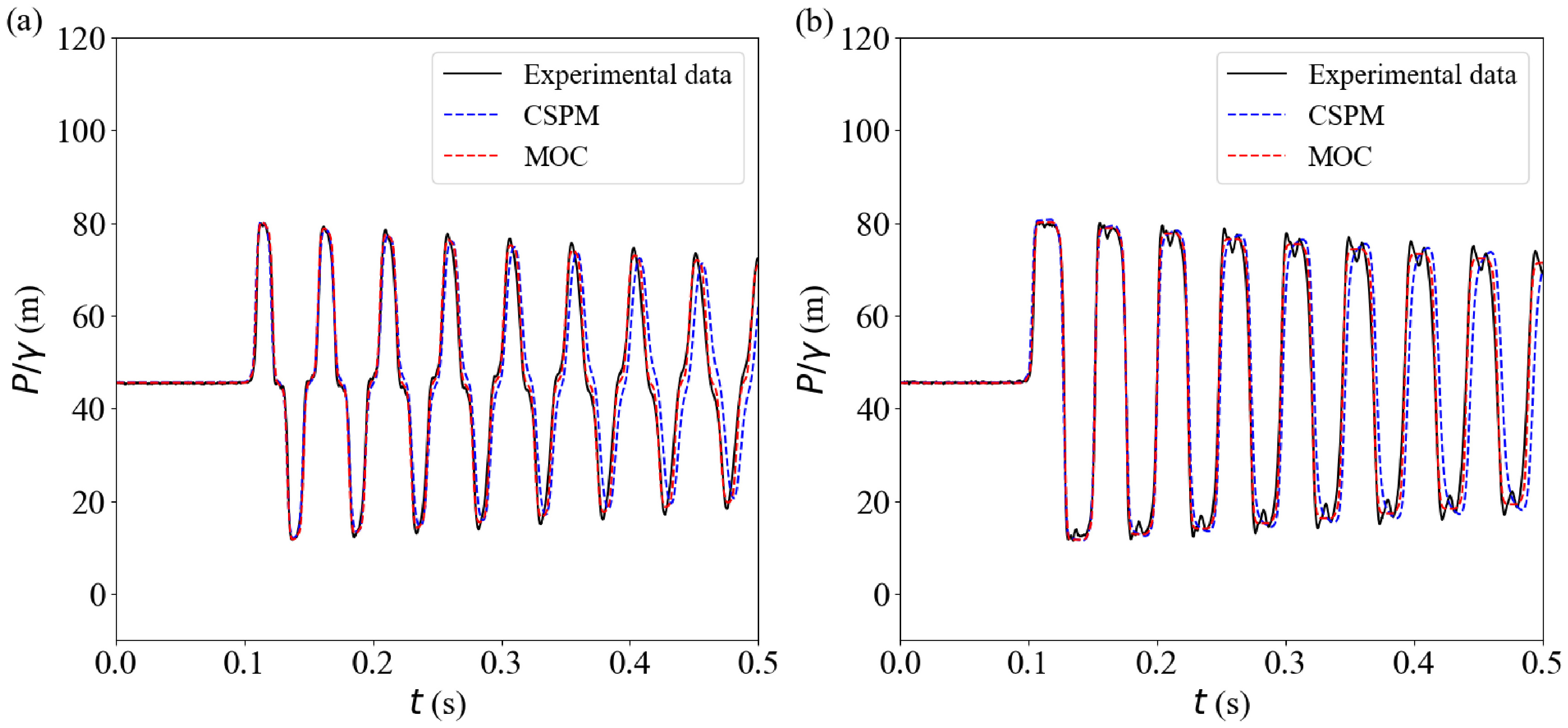
Results obtained by CSPM are compared with results from MOC and experimental data in Figures 1 and 2. A set of 305 evenly distributed particles were used in the simulations. The time-step increment was calculated using the Courant number formula, $\Delta \text{t =}\Delta \text{x/a = 3}{\text{.98 x 10}}^{\text{-5}}\text{s}$. For the constant coefficients, the following values were used: $\alpha \text{= 1}\text{.0}$; $\beta \text{= 2}\text{.0}$; $\eta \text{= 0}\text{.01}$; pp = 0.5. The smoothing length $\text{h = 1}\text{.0}\Delta \text{x}$was used (Hou et al., 2012). In MOC, the time-step incrementation was $\Delta \text{t = 7}{\text{.97 x 10}}^{\text{-4}}\text{s}$.

Figure 1
Transient pressure traces versus CSPM and Moc results for Q_o = 85 x 10-⁶ m³ s^-1: (a) middle pipe section and (b) valve section.

Figure 2
Transient pressure traces versus CSPM and Moc results for Qo = 133 x 10-6 m3 s-1: (a) middle pipe section and (b) valve section.

The root-mean-square-errors (RMSE) calculated for Scenario1 are as follows: RMSE_{MOC_85_middle} = 2.03 m; RMSE_{MOC_85_valve} = 2.33 m; RMSE_{CSPM_85_middle} = 6.22 m; RMSE_{CSPM_85_valve} = 8.80 m. For Scenario 2, the following values were obtained: RMSE_{MOC_133_middle} = 2.33 m; RMSE_{MOC_133_valve} = 1.64 m; RMSE_{CSPM_133_middle} = 7.63 m; RMSE_{CSPM_133_valve} = 10.77 m.

Results in Figures 1 and 2 demonstrate that both methods may accurately reproduce the amplitude of the pressure wave, in which no smearing effect is visible. Nevertheless, as the transient event progresses, slightly differences in period are obtained (phase errors), especially in CSPM. This behavior may be explained by several factors (Pan et al., 2022; Violeau & Rogers, 2016): the assumption that wave speed is constant during numerical simulations; the neglection of the fluid-structure interaction effect. The results also show that the pre-smoothing technique was able to eliminate pressure overshoot at the first pressure wave front.

To evaluate the maximum and minimum head pressures in the initial 0.5 s of simulation, Table 2 was generated. It shows that both CSPM and MOC were able to reproduce the values obtained in experimental data.

Table 2
Compilation of results for the comparison between MOC, CSPM, and experimental data for the initial 0.5 s of simulation.

Qo (m3/s)	Maximum head pressure (m)			Minimum head pressure (m)
	MOC	CSPM	Experimental data	MOC	CSPM	Experimental data
85x10-6	80.20	80.75	80.26	11.63	11.47	11.44
133x10-6	98.71	99.39	99.24	-8.46	-8.84	-7.62

Influence of particle number

To evaluate the influence of particle number in CSPM simulations, Scenario 1 was used with three different configurations: N = 305, N = 153, and N = 31. Figure 3 shows that fewer particles tend to generate more numerical dissipations of pressure oscillations. This behavior may be explained by the larger truncation error in the kernel approximation of the spatial derivatives when fewer particles are used (Pan et al., 2022). It also reveals the smearing effect, which becomes less significant when more particles are employed (Hou et al., 2012).

Figure 3
Influence of the particle number in CSPM results. Valve section.

Influence of the smoothing function

To evaluate the influence of the smoothing function in CSPM simulations, Scenario 1 was used with N = 153. Two kernels were used: the one-dimensional cubic spline and the modified gaussian. Figure 4 shows that both functions predicted the pressure history at the valve well. Nevertheless, it is hard to determine which one is optimum for different scenarios, since it depends on the specific meshfree method and problem (Hou et al., 2012).

Figure 4
Influence of the smoothing function. Valve section.

Figure 4 also provides evidence to explain the computational efficiency of the cubic spline function and its wide use in CSPM simulations (Monaghan & Lattanzio, 1985; Hou et al., 2012; Pan et al., 2022).

Influence of artificial viscosity and the parameters $\text{α}$ and $\text{β}$

Artificial viscosity is a dissipative term utilized to suppress numerical wiggles, dissipate high free frequency energy and stabilize numerical scheme (Hou et al., 2012; Pan et al., 2022). To evaluate its influence in CSPM simulations, Scenario 1 was used with N = 153. Figure 5 demonstrates the numerical oscillations generated by the absence of the term.

Figure 5
Influence of artificial viscosity in CSPM results. Valve section.

Another two simulations were conducted to evaluate the influence of the artificial viscosity parameters ($\text{α}$ and $\text{β}$). In the first one, $\text{β}$ = 2.0 and $\text{α}$ was tested for three different values (0.5, 1.0, and 1.5). Figure 6 shows that numerical dissipations of transient pressures tend to become higher once $\text{α}$ increases from 0.5 to 1.5. In this way, the parameter may relieve the numerical oscillation (Pan et al., 2022).

Figure 6
Influence of parameter $\text{α}$ with fixed $\text{β}$ = 2.0. Valve section.

In the last simulation, $\text{α}$ = 1.0 and $\text{β}$ was tested for three different values (1.0, 2.0, and 3.0). Figure 7 shows that the results maintain consistency independently of the value used for $\text{β}$. It happens due to the insignificant influence of the term $\beta {\text{u}}_{\text{ij}}^{\text{2}}$ in Equation 21, once the Mach number is small (Pan et al., 2022). As discussed previously, this term is used to restrain particle interpenetration at high Mach numbers.

Figure 7
Influence of parameter $\text{β}$ with fixed $\text{α}$ = 1.0. Valve section.

Influence of unsteady friction losses

To evaluate the influence of UFM in CSPM simulations, Scenario 1 was used with N = 153. Figure 8 shows that the computation of unsteady friction losses generates more accurate results. In addition, it contributes to the matching between numerical results and experimental data in terms of shift and shape of the pressure wave (Soares et al., 2017).

Figure 8
Influence of UFM in CSPM results in the first pressure waves. Valve section

Another simulation was conducted to evaluate the influence of UFM in CSPM during the first second of simulation. Scenario 1 was used with N = 153. Figure 9 shows that the absence of unsteady friction losses tend to generate higher amplitude waves, which postpones the transient dissipation. In contrast, UFM is able to reproduce the wave amplitude observed in experimental data.

Figure 9
Influence of UFM in CSPM results in the first second of simulation. Valve section.

Influence of the pre-smoothing parameter

To evaluate the influence of the pre-smoothing parameter in CSPM simulations, Scenario 1 was used with N = 153. The parameter pp was simulated for two different values: 0.0, which results in no pre-smoothing and no correction on the particle velocity; 0.5, which indicates the correction of the particle velocity by the mean velocity of the particles contained in its compact support. Figure 10 shows pressures overshoots at the wave fronts when no pre-smoothing is applied (pp = 0.0). In contrast, the results with pre-smoothing (pp = 0.5) indicate no overshoots and smooth pressure waves.

Figure 10
Influence of the pre-smoothing parameter in CSPM. Valve section.

CONCLUSIONS

This research presents numerical analyses of transient flow in a horizontal straight copper pipe. Experimental data of transient events caused by rapid valve closure in turbulent conditions was used. CSPM (meshfree) and MOC (mesh based) were implemented with UFM. Stability and accuracy of both methods were analyzed. The main conclusions are as follows:

• Both CSPM and MOC are able to accurately reproduce the amplitude of the pressure wave. Nevertheless, phase errors are visible as the transient event progresses. The common causes of these problems are the assumption of constant wave speed during the transient flow and the neglection of the fluid-structure interaction effect;

• Although the methods have presented similar results, RMSE indicates that MOC leads to more accurate values for the cases analyzed;

• Setting the particle number in CSPM is essential to guarantee the method’s stability. Fewer particles tend to generate more numerical dissipations of pressure oscillations, which may be explained by the truncation error in the kernel approximation of the spatial derivatives when fewer particles are used (Pan et al., 2022). It also reveals the smearing effect, which becomes less significant when more particles are employed (Hou et al., 2012);

• It is impossible to determine an optimum smoothing function for CSPM simulations, since it depends on the specific meshfree method and problem (Hou et al., 2012). However, the results provided evidence to explain the computational efficiency of the cubic spline function and its wide use in CSPM simulations (Monaghan & Lattanzio, 1985; Hou et al., 2012; Pan et al., 2022);

• Artificial viscosity is necessary to suppress numerical wiggles, dissipate high free frequency energy and stabilize numerical scheme (Hou et al., 2012; Pan et al., 2022). Results indicate that numerical dissipations of transient pressures tend to become higher once $\text{α}$ increases from 0.5 to 1.5. In this way, the parameter may relieve the numerical oscillation (Pan et al., 2022). In contrast, $\text{β}$ has insignificant influence on the results, once the Mach number is small (Pan et al., 2022);

• Considering unsteady friction losses in the simulations contributes to the matching between numerical results and experimental data in terms of shift and shape of the pressure wave (Soares et al., 2017);

• The pre-smoothing parameter is essential to prevent pressure overshoots at the wave fronts. It works based on the correction of the particle velocity using the velocities of the particles contained in its compact support, scaled by pp.

NOTATION

A = pipe cross-sectional area (m²)

a = elastic wave speed (m/s)

${\text{A}}_{\text{i}}$, A₁, A₂, ${\text{B}}_{\text{i}}$, B₁, B₂ = coefficients in shear stress formulae (-)

D = pipe inner diameter (m)

f = Darcy-Weisbach friction factor (-)

f^*= Fenning friction factor (-)

g = gravity acceleration (m/s²)

H_r = steady-state pressure head at the upstream reservoir (m)

h, h_i, h_j= smoothing length, smoothing length of particles i and j (m)

${\overline{h}}_{\text{ij}}$ = average smoothing length associated with particles i and j (m)

m_j = mass of particle j (kg)

N = particle number (-)

P, P_i = pressure, pressure of particle i (Pa)

Pⁿ, Pⁿ⁺¹ = pressure at time n$\Delta \text{t}$ and (n + 1)$\Delta \text{t}$ (Pa)

P/$\text{γ}$ = pressure head (m)

pp = parameter of pre-smoothing (-)

Q_o = steady-state discharge (m³/s)

R = distance between two particles scaled by the smoothing length (-)

R_e = Reynolds number (-)

S_i = set of particles that form the compact support of the particle i (-)

t = time (s)

V, V_i, V_j = mean flow velocity, velocity of particles i and j (m/s)

Vⁿ, Vⁿ⁺¹ = velocity at time n$\Delta \text{t}$ and (n + 1)$\Delta \text{t}$ (m/s)

V_t, V_t-$\Delta \text{t}$ = velocity at time t and (t-$\Delta \text{t}$) (m/s)

W, ${\text{W}}_{\text{ij}}$ = smoothing functions (-)

x, x_i, x_j = coordinate along pipe axis, coordinate along pipe axis of particles i and j (m)

${\text{Y}}_{\text{i}}$, ${\text{Y}}_{\text{1}}$, ${\text{Y}}_{\text{2}}$ = functions of time (-)

$\text{α}$, $\text{β}$, and $\text{η}$= artificial viscosity constant coefficients (-)

$\text{γ}$ = specific weight (N/m³)

$\Delta \text{t}$ = time-step increment (s)

$\Delta \text{x}$ = space-step (m)

$\text{μ}$ = dynamic viscosity (kg/ms)

$\text{ν}$ = kinematic viscosity (m²/s)

${\Pi }_{\text{ij}}$ = artificial viscosity between particles i and j (-)

$\text{ρ}$, ${\text{ρ}}_{\text{j}}$ = fluid density, density of particle j (kg/m³)

$\text{τ}$, ${\text{τ}}_{\text{s}}$, ${\text{τ}}_{\text{u}}$= wall shear stress, steady and unsteady components of wall shear stress (Pa)

$\Psi$ = non-dimensional time (-)

$\Omega$ = surface and domain (-)

ACKNOWLEDGEMENTS

The first author gratefully acknowledges the financial support of the Coordenação de Aperfeiçoamento de Pessoal de Nível Superior – Brasil (CAPES).

DATA AVAILABILITY STATEMENT

Research data is only available upon request.

REFERENCES

• Agostinho, M. S. P., & Fernandes, C. V. S. (2024). Understanding the discoloration risk as consequence of hydraulic transients. RBRH, 29(15), 1-12. https://doi.org/10.1590/2318-0331.292420240011
  » https://doi.org/10.1590/2318-0331.292420240011
• Chaudhry, M. H. (2014). Applied hydraulic transients (3rd ed.). New York: Springer. https://doi.org/10.1007/978-1-4614-8538-4
  » https://doi.org/10.1007/978-1-4614-8538-4
• Chen, J. K., Beraun, J. E., & Carney, T. C. (1999). A corrective smoothed particle method for boundary value problems in heat conduction. International Journal for Numerical Methods in Engineering, 46(2), 231-252. https://doi.org/10.1002/(SICI)1097-0207(19990920)46:2<231::AID-NME672>3.0.CO;2-K
  » https://doi.org/10.1002/(SICI)1097-0207(19990920)46:2<231::AID-NME672>3.0.CO;2-K
• Chen, J. K., Beraun, J. E., & Jih, C. J. (2001). A corrective smoothed particle method for transient elastoplastic dynamics. Computational Mechanics, 27(3), 177-187. https://doi.org/10.1007/s004660100236
  » https://doi.org/10.1007/s004660100236
• Colagrossi, A. (2004). A meshless lagrangian method for free–surface and interface flows with fragmentation Roma: Università di Roma La Sapienza.
• Gingold, R. A., & Monaghan, J. J. (1977). Smoothed particle hydrodynamics: theory and application to non-spherical stars. Monthly Notices of the Royal Astronomical Society, 181(3), 375-389. https://doi.org/10.1093/mnras/181.3.375
  » https://doi.org/10.1093/mnras/181.3.375
• Hou, Q., Kruisbrink, A. C. H., Tijsseling, A. S., & Keramat, A. (2012). Simulating water hammer with corrective smoothed particle method. In S. Anderson (Ed.), Proceedings of the 11th International Conference on Pressure Surges (pp. 171-187). Cranfield: BHR Group.
• Hou, Q., Wang, S., Kruisbrink, A. C. H., & Tijsseling, A. S. (2015, November). Lagrangian modelling of fluid transients in pipelines with entrapped air. In Proceedings of the 12th International Conference on Pressure Surges (pp. 215-227), Dublin. Cranfield: BHR Group.
• Liu, G. R., & Liu, M. B. (2003). Smoothed particle hydrodynamics: a meshfree particle method Singapore: World Scientific Connect. https://doi.org/10.1142/5340
  » https://doi.org/10.1142/5340
• Liu, M. B., & Liu, G. R. (2010). Smoothed Particle Hydrodynamics (SPH): an overview and recent developments. Archives of Computational Methods in Engineering, 17(1), 25-76. https://doi.org/10.1007/s11831-010-9040-7
  » https://doi.org/10.1007/s11831-010-9040-7
• Lucy, L. B. (1977). A numerical approach to the testing of the fission hypothesis. The Astronomical Journal, 82(12), 1013. https://doi.org/10.1086/112164
  » https://doi.org/10.1086/112164
• Martins, N. M. C., Soares, A. K., Ramos, H. M., & Covas, D. I. C. (2016). CFD modelling of transient flow in pressurized pipes. Computers & Fluids, 126, 129-140. https://doi.org/10.1016/j.compfluid.2015.12.002
  » https://doi.org/10.1016/j.compfluid.2015.12.002
• Monaghan, J. J., & Gingold, R. A. (1983). Shock simulation by the particle method SPH. Journal of Computational Physics, 52(2), 374-389. https://doi.org/10.1016/0021-9991(83)90036-0
  » https://doi.org/10.1016/0021-9991(83)90036-0
• Monaghan, J. J., & Lattanzio, J. C. (1985). A refined particle method for astrophysical problems. Astronomy & Astrophysics, 149(1), 135-143.
• Monaghan, J. J. (1997). SPH and riemann solvers. Journal of Computational Physics, 136(2), 298-307. https://doi.org/10.1006/jcph.1997.5732
  » https://doi.org/10.1006/jcph.1997.5732
• Oliveira, L. C. S., & Lima Neto, I. E. (2025). The impacts of the water intake operation on the hydraulic transients, sediment resuspension and water quality of the largest multi-use reservoir in Latin America. RBRH, 30(6), 1-9. https://doi.org/10.1590/2318-0331.302520240093
  » https://doi.org/10.1590/2318-0331.302520240093
• Pan, T., Zhou, L., Ou, C., Wang, P., & Liu, D. (2022). Smoothed particle hydrodynamics with unsteady friction model for water hammer pipe flow. Journal of Hydraulic Engineering, 148(2), 04021057. https://doi.org/10.1061/(ASCE)HY.1943-7900.0001966
  » https://doi.org/10.1061/(ASCE)HY.1943-7900.0001966
• Shepard, D. (1968). A two-dimensional interpolation for irregularly-spaced data function. In R. B. Blue, & A. M. Rosenberg (Eds.), Proceedings of the 1968 23rd ACM national conference (pp. 517-524). New York: ACM. https://doi.org/10.1145/800186.810616
  » https://doi.org/10.1145/800186.810616
• Silva, J. V. V., Sierra, D. A., Sodek, D. B., Martim, A. L. S. S., Dalfré Filho, J. G., & Luvizotto Junior, E. (2024). Proposal of resilience indices for water mains subject to hydraulic transients and case study in Franca (Brazil). RBRH, 29(42), 1-12. https://doi.org/10.1590/2318-0331.292420240002
  » https://doi.org/10.1590/2318-0331.292420240002
• Soares, A. K., Martins, N. M. C., & Covas, D. I. C. (2017). Transient vaporous cavitation in a horizontal copper pipe. Journal of Hydraulic Research, 55(5), 731-736. https://doi.org/10.1080/00221686.2017.1286394
  » https://doi.org/10.1080/00221686.2017.1286394
• Vardy, A. E., & Hwang, K. L. (1993). A weighting function model of transient turbulent pipe friction. Journal of Hydraulic Research, 31(4), 533-548. https://doi.org/10.1080/00221689309498876
  » https://doi.org/10.1080/00221689309498876
• Violeau, D., & Rogers, B. D. (2016). Smoothed particle hydrodynamics (SPH) for free-surface flows: past, present and future. Journal of Hydraulic Research, 54(1), 1-26. https://doi.org/10.1080/00221686.2015.1119209
  » https://doi.org/10.1080/00221686.2015.1119209
• Wylie, E. B., & Streeter, V. L. (1993). Fluid transients in systems Englewood Cliffs, NJ: Prentice Hall.
• Zhang, C., Zhu, Y., Wu, D., Adams, N. A., & Hu, X. (2022). Smoothed particle hydrodynamics: methodology development and recent achievement. Journal of Hydrodynamics, 34(5), 767-805. https://doi.org/10.1007/s42241-022-0052-1
  » https://doi.org/10.1007/s42241-022-0052-1
• Zhao, M., & Ghidaoui, M. S. (2004). Godunov-type solutions for water hammer flows. Journal of Hydraulic Engineering, 130(4), 341-348. https://doi.org/10.1061/(ASCE)0733-9429(2004)130:4(341)
  » https://doi.org/10.1061/(ASCE)0733-9429(2004)130:4(341)

Edited by

• Editor-in-Chief:
  Adilson Pinheiro

• Associated Editor:
  Fábio Veríssimo Gonçalves

Publication Dates

• Publication in this collection
  07 Aug 2026
• Date of issue
  2026

History

• Received
  06 Oct 2025
• Reviewed
  31 Mar 2026
• Accepted
  11 June 2026