Physical and stochastic modeling of trap efficiency in reservoirs

Modelagem física e estocástica da eficiência de retenção em reservatórios

ABSTRACT

Reservoir sedimentation is a critical issue affecting the operational lifespan and storage capacity of hydraulic structures. In this context, Trap Efficiency (TE) is a key parameter used to quantify the ability of a reservoir to retain incoming sediments. The calculation of Trap Efficiency is traditionally performed to estimate siltation in reservoirs. Thus, the objective of this paper was to perform physical and stochastic modeling of TE in reservoirs. For this purpose, siltation was a simulated in a reduced model of a reservoir model using five different flow series generated stochastically. At the end of the simulations, TE values were obtained experimentally and compared with those calculated using the methods of Churchill, Brune and Heinemann. The latter two showed the best results. Using the stochastically generated flows, thousands of TE values were calculated with the three empirical methods. In this case, the Heinemann method showed better results. Thus, the calculated TE can vary according to the flow series used, even when they correspond to the same period and share the same mean and standard deviation. Therefore, stochastic modeling can help in selecting the most appropriate method for calculating the TE.

Keywords:
Brune; Churchill; Heinemann; Silting; Flow

RESUMO

A sedimentação em reservatórios é um problema crítico que afeta a vida útil operacional e a capacidade de armazenamento de estruturas hidráulicas. Nesse contexto, a Eficiência de Retenção (ER) é um parâmetro fundamental utilizado para quantificar a capacidade de um reservatório em reter os sedimentos afluentes. O cálculo da Eficiência de Retenção é tradicionalmente realizado para estimar o assoreamento em reservatórios. Assim, o objetivo deste trabalho foi realizar modelagem física e estocástica da ER em reservatórios. Para isso, o assoreamento foi simulado em um modelo reduzido de reservatório utilizando cinco diferentes séries de vazões geradas estocasticamente. Ao final das simulações, os valores de ER foram obtidos experimentalmente e comparados com aqueles calculados pelos métodos de Churchill, Brune e Heinemann. Os dois últimos apresentaram os melhores resultados. Utilizando as vazões geradas estocasticamente, milhares de valores de ER foram calculados com os três métodos empíricos. Nesse caso, o método de Heinemann apresentou melhores resultados. Assim, a ER calculada pode variar de acordo com a série de vazões utilizada, mesmo quando estas correspondem ao mesmo período e apresentam a mesma média e desvio padrão. Dessa forma, a modelagem estocástica pode auxiliar na seleção do método mais adequado para o cálculo da ER.

Palavras-chave:
Brune; Churchill; Heinemann; Assoreamento; Vazão

INTRODUCTION

The reservoirs are of great economic importance in the country, therefore, studies before their construction are relevant. Santos & Cunha (2015) reported that the analysis of the implementation of a reservoir must consider economic and environmental feasibility, and the costs of its conservation. When the reservoirs are fully silted, they lose their functionality, as the removal of sediment is often impossible due to economic factors. Thus, the main function of the reservoir is only guaranteed when studying sedimentation (Morris, 2020). In this regard, it is necessary to create scenarios that estimate how the reservoir will behave over time, in order to assess its siltation and, consequently, its loss of reserve volume and useful life.

Silting can be described as a natural process where sediments present in the river flow are deposited due to a reduction in the affluent velocity, as well as the transport capacity (Valent et al., 2019). Alighalehbabakhani et al. (2017) pointed out that this phenomenon has been intensifying with human intervention. Advanced land use and management, intensive, unsustainable, and unbalanced human activities, agricultural and urban expansion to regions with high erosion proneness as well as other anthropogenic activities, increase erosion, which causes an escalation in sedimentation, becoming increasingly important to study this phenomenon.

The prediction of siltation is something that has been studied for a long time and has several different approaches (Hager, 2018). The choice of the best method to be used is a factor for discussion by several authors. Depending on the hydrographic basin, there is a better adaptation or not of the proposed formulas and software. Sultana & Naik (2015) described the wide range of sedimentation calculation methods, each of which has its own complexity and input data.

One of the most important ways of estimating siltation is through the Trap Efficiency (TE), which is a parameter that measures the reservoir's capacity to retain the sediments affluent to it. For this, there are two methods of calculation: the theoretical and the empirical. The second is the most widely used, as they are prompt, simple, and with fewer input data (Issa et al., 2015). More recently, numerical 2D sediment transport models have also been applied to quantify sediment retention in Brazilian river confluences, with retention efficiencies of approximately 50% reported during extreme flood events in Minas Gerais (Marciano et al., 2024).

Revel et al. (2015) present the widely used empirical models of Brune and Churchill, and the Heinemann method. In addition, the authors comment on its use limitations as they consider few hydro-sedimentological parameters in their formulas, which interferes with the final result. The absence of these parameters limits the applicability of the formulation, preventing it from being reliably applied to reservoirs whose physical characteristics differ from those considered during model calibration. Thus, it appears that the empirical models were elaborated considering some reservoirs in specific regions, which may not be suitable for other regions with different characteristics (Tan et al., 2019).

In addition, these empirical approaches do not explicitly account for the characteristics of the incoming sediment, such as grain size distribution, density, and sediment origin. Furthermore, they do not incorporate structural aspects of the reservoir, including spillway configuration and water intake structures, which may significantly influence sediment retention dynamics. These aspects should therefore be recognized as inherent limitations of the method.

Li et al. (2018) in their studies on silting in reservoirs addressed three different reinterpretations of the Brune and Heinemann model. All obtained satisfactory results, where each curve adjusted to a reservoir with particular and distinct characteristics. Obreja (2012) estimated the TE for 14 reservoirs in the Siret watershed in Romania using Brune's model. The author reported an agreement ranging from 42% to 98% between calculated and observed values in the analyzed reservoirs. It was also observed that the Brune model is correlated with reservoir capacity: for large reservoirs, TE values tend to approach 100%, whereas for smaller reservoirs, TE decreases.

Sultana & Naik (2015) tested some empirical methods and obtained satisfactory results with Brune's. Issa et al. (2015), using six different methods to estimate the TE in the Mosul Dam reservoir, Israel, observed a good agreement of the real value with those calculated using all methods, with the greatest variation of this parameter being less than 4%. For the Tehri reservoir, India, Garg et al. (2020) studied their TE. In their paper, the empirical methods used were those of Brune and Churchill, where Brune's method overestimated the TE value of the reservoir.

One way to evaluate empirical methods for estimating the TE is through physical modeling. This type of model facilitates the control of the quantities to be considered (Teixeira et al., 2020) so that the result obtained tends to be more accurate, as long as the scales of hydraulic similarity between the model and the prototype are respected. Thus, with a structure that simulated a reservoir, Revel et al. (2015) compared the methods of Churchill and Brune calculation with the observed experimental results. They concluded that none of the equations came close to what was observed, as both overestimated the values obtained since more than 50% of the observed values were below both curves.

One of the main input parameters in the methods that estimate the TE is the flow. It should be noted that the value of this parameter commonly has uncertainties, especially in developing countries (Mulu & Dwarakish, 2015). Maldonado et al. (2015) stated that each flow measurement method has its inaccuracies. For example, one of the ways used in reservoirs is to obtain the flow value through key curves. This method allows the measurement of flow through an equation that relates it to the linimetric height. The bases of this function are the flow and height data collected in times of drought and floods (Araújo et al., 2017). This methodology, being mostly manual, leads to several built-in errors.

It should be noted, however, that the uncertainties associated with discharge measurements based on rating curves are more significant in riverine environments. In contrast, in water supply and hydropower reservoirs, flow measurements are often obtained using high-accuracy instrumentation, such as flow meters and controlled hydraulic structures. Therefore, the magnitude of uncertainty in discharge data may be lower in such systems than that suggested by studies focused on natural channels.

Coz et al. (2012) pointed out that without the evaluation of uncertainties, the user can have potential errors when using flow data, which can compromise the accuracy of hydraulic models. Thus, without an assessment of the uncertainties contained in the input parameters of the methods, the estimated values for the TE can have significant errors. Therefore, an assessment of how much a change in flow interferes with the TE is extremely important.

To assess the influence of flow variation on TE values, stochastic methods can be used, which allow considering the uncertainties involved in the values of input parameters, such as flow. Therefore, some authors proposed stochastic methods for simulating siltation in reservoirs, such as Guo et al. (2018), Schleiss et al. (2016), and Shrestha et al. (2016). However, it was not found any work in the literature that used a stochastic model to assess the sensitivity of empirical TE estimation methods for flow variation.

Given the above, the objective and originality of this paper are (i) to evaluate how much the variation in the inflow to the reservoir interferes with the Trap Efficiency (TE) value. In addition, the objective is (ii) to compare the Trap Efficiency values of the empirical models (Brune, Churchill, and Heinemann) against the values observed in the small scale model of a reservoir and; (iii) define which of these empirical models best fit the physical model.

METHODOLOGY

Empirical trap efficiency estimation methods

According to Revel et al. (2015), few studies on sedimentation in reservoirs have been reported in the literature, which most of these are based on analytical methods. In general, the amount of sediment accumulated inside a reservoir is directly and closely related to its Trap Efficiency (TE). The TE is defined as the ratio between the portion of sediment that is retained within the reservoir and the volume affluent to it, as presented in Equation 1.

$\text{TE =}\frac{{\text{V}}_{inflow}{\text{- V}}_{outflow}}{{\text{V}}_{inflow}}$ (1)

Where, ${\text{V}}_{\text{inflow}}$ is the volume of sediment entering a reservoir (m³); ${\text{V}}_{\text{outflow}}$ is the volume of sediment leaving a reservoir (m³).

Based on this assumption, several authors created empirical models to estimate the TE. Van Rijn (2013) in his work addressed the curve developed by Brune, who used data from 40 reservoirs with large reserve capacity located in the US that are normally full (reservoirs fully filled with water and which had an outlet on the upper edge). The curve is dependent on the reservoir's total reserve capacity and its annual inflow volume.

Several authors have developed empirical models to estimate TE. Brune (1953) used data from 40 typically full reservoirs in the United States, featuring spillways located at the upper edge. This curve depends on the total storage capacity of the reservoir and its annual inflow volume, as expressed in Equation 2.

$TE=\frac{0.000085+{\left(\frac{V}{Vw}\right)}^{1.1}}{0.0085+{\left(\frac{V}{Vw}\right)}^{1.1}}$ (2)

Where, $V$ is the reservoir capacity (m³); and $V_w$ is the reservoir’s average annual inflow volume (m³).

More recently, Rabelo et al. (2025) applied Brune's sediment retention index to eight reservoirs in the Brazilian semi-arid region, confirming its applicability across systems with drainage areas ranging from 44 to 1,519 km², with observed sedimentation rates consistent with the method's predictions.

Heinemarm (1981) modified the relationship between TE and the Brune parameter V/Vw, using data from 20 typically full small agricultural reservoirs (Verstraeten & Poesen 2000). The model proposed by Heinemann is presented in Equation 3.

$TE=-22+\frac{119.6\frac{V}{Vw}}{0.012+\left(1.02\frac{V}{Vw}\right)}$ (3)

Churchill (1948) utilized data from reservoirs located in the Tennessee Valley region, USA. The method consists of calculating the Sedimentation Index, given by Equation 4.

$SI=\frac{V^2}{Q^{2}L}$ (4)

Where, $SI$ is the reservoir sedimentation index (s²/m); $Q$ is the average daily inflow discharge during the study period (m³/s); $L$ is the reservoir length (m).

With IS, it is possible to calculate the percentage of sediments that outflow from the reservoir (SE), which is a parameter antagonistic to TE. SE is given by Equation 5.

$$SE=100-\left(112-1013.4\cdot I{S}^{-0.2}\right)$$ (5)

Where, $SE$ is the percentage of sediments outflowing from the reservoir (%). Thus, the sediment TE is obtained by subtracting $SE$ from 100%.

This method is recommended for small reservoirs with volumes below 10 hm³ (Carvalho 2008). However, studies have demonstrated the applicability of the model to large reservoirs as well, such as the John Martin Reservoir (744.41 hm³) (Borland, 1971, as cited in Verstraeten & Poesen, 2000). This suggests that the method’s performance is related not only to the reservoir volume but also to sediment characteristics, including their origin and grain size distribution.

Also noteworthy is the complexity of the Sedimentation Index, especially in tropical contexts, where the estimate of average flow becomes less reliable (Garg et al., 2020). As a result, the TE calculated by the Churchill method can show high variability and is sensitive to the specific conditions of each reservoir.Heinemann, for small agricultural reservoirs with tributary areas ranging from 0.8 to 36.3 km², proposed modifications in the relationship between TE and Brune's V/Vw parameter, using data from 20 normally full reservoirs (Verstraeten & Poesen, 2000).

Carvalho (2008) presented another way to estimate the TE. This was proposed by Churchill who used data from small reservoirs located in the Tennessee Valley region, USA, one of the parameters being the average daily flow. The first point for using this method is the calculation of the Sedimentation Index (SI).

With the SI it is possible to calculate the percentage of sediment that outflow from the reservoir (SE), which is an antagonistic parameter to TE, but necessary for the calculation.

Small scale physical model description

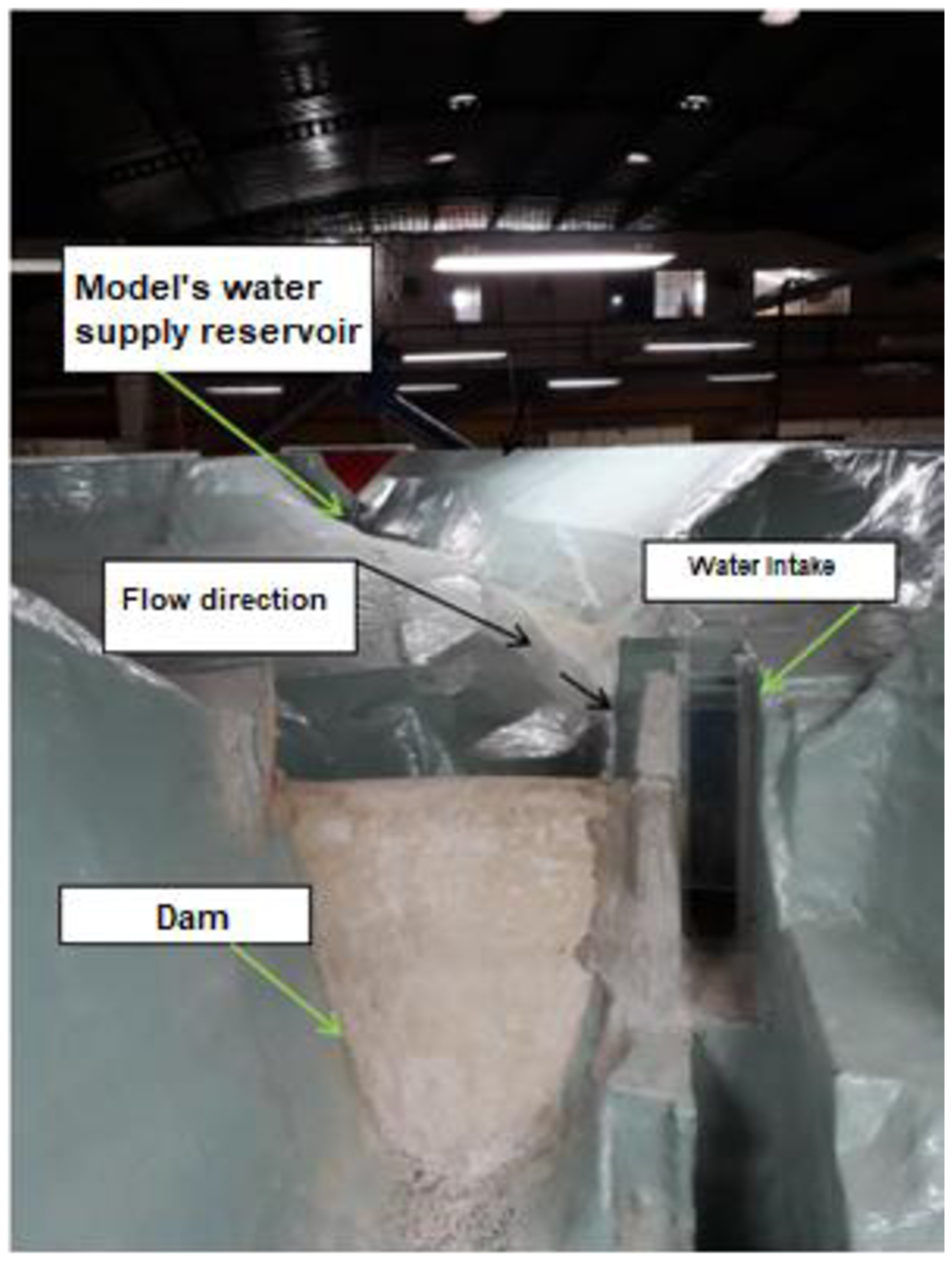
The small scale physical model (Figure 1) used in this study is located at the Center for Hydraulic Research (CPH) of the Federal University of Minas Gerais (UFMG) and it is a representation of the Salto Paraopeba Small Hydropower Plant (PCH) (Jeceaba-MG). Its length is 10m upstream of the dam, which corresponds to 1000m in the prototype. Its volumetric reserve capacity, considering the normal level of operation of the reservoir is 2.88 m³, which, according to the volume scale between model and prototype, corresponds to 0.711 hm³ in the real reservoir. All constructive details, design assumptions and design calculations of the small scale model can be verified in the work of Carvalho et al. (2014).

Figure 1
Front view of the small scale model of the PCH.

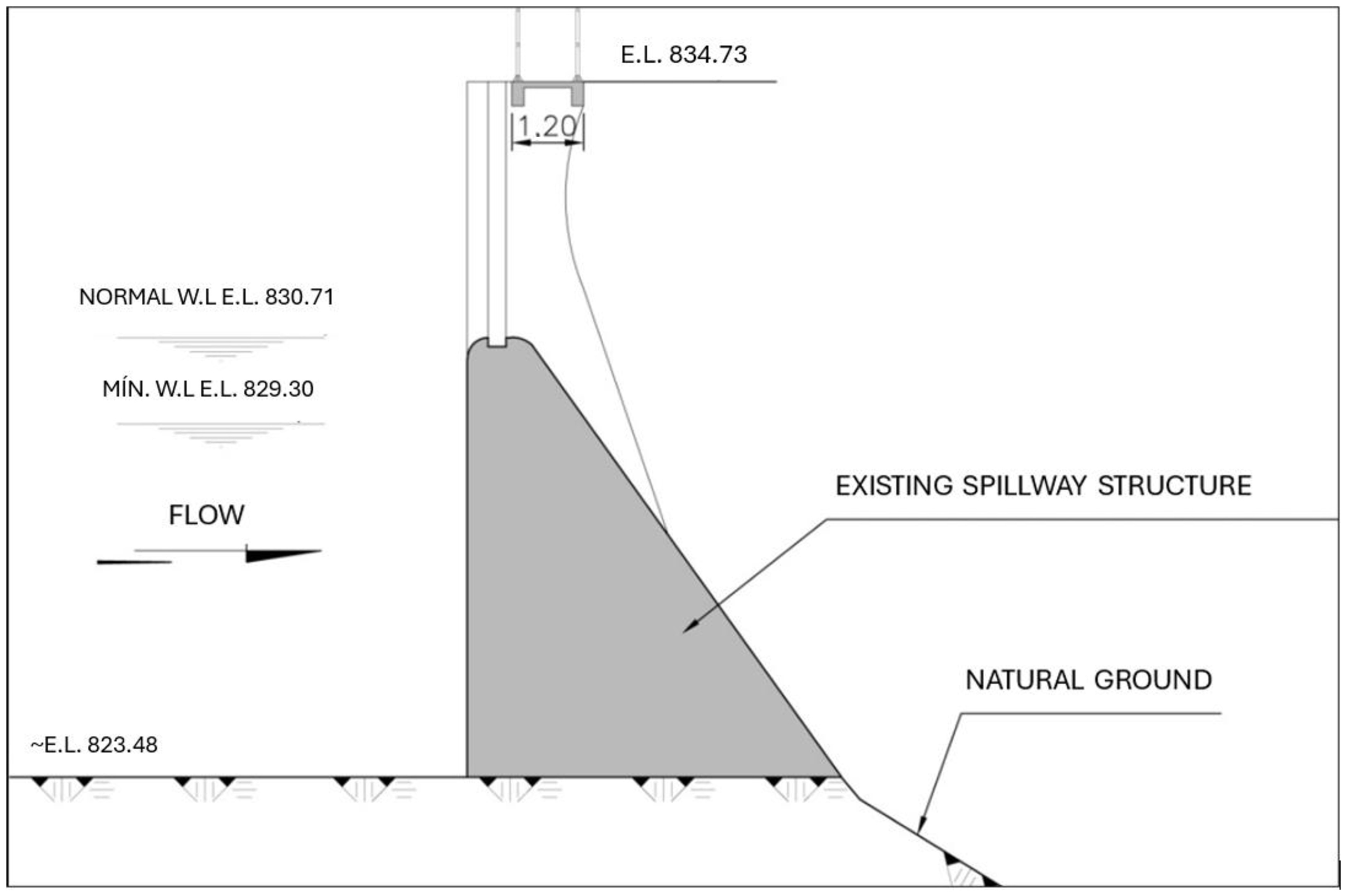
Figure 2 presents a general layout of the PCH Salto Paraopeba dam, indicating the location, type and crest elevation of the spillway and water intake structures, as well as the normal and maximum water levels.

Figure 2
Layout model of the PCH.

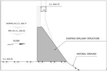
Table 1 presents the main attributes of the physical model used to determine the TE (Carvalho et al., 2014).

Table 1
Adopted scales in the design of the reduced-scale model of the SHP.

Quantity	Scale	Real Value	Model Value
Length	99.3	1200 m	12.1 m
Width	99.3	600 m	6.0 m
Depth	25.0	30.0 m	1.2 m
Grain diameter	0.40	0.45 mm	1.13 mm
Time	2.48	5 years	17.60 h
Froude number	1	1	1
Reynolds number	125	2.000	16.0
Reynolds grain number	1	1	1
Shields Parameter	1	1	1
Darcy-Weisbach Friction Factor	0.25	0.25	1
Sedimentation velocity	2.5	7.9 cm/s	3.1 cm/s
Sediment density	15.8	2.7	1.1

Stochastic generation of flow values used in the small scale model

In order to evaluate the influence of the uncertainties in the flow values on the TE result, stochastic series of flows were generated using the AR(1) stochastic method, which is given by Equation 6.

${\text{Q}}_{\text{t}}\text{=}\overline{Q}\text{+}\varphi {\text{(Q}}_{\text{t-1}}\text{-}\overline{Q}\text{)+}{\sigma }_{\text{x}}{\epsilon }_{\text{t}}\sqrt{\text{1-}{\varphi }_{\text{1}}^{\text{2}}}$ (6)

Where, $Q_t$ is the annual flow for the time t of interest (m³/s); $\overline{Q}$ is the average of the observed data of the temporal series of flows (m³/s); $\varphi$ is the lag 1 autocorrelation coefficient of the temporal series of flows; ${\sigma }_x$ is the standard deviation of the temporal series of flows; ${\epsilon }_i$ is the randomness component generated from the normal distribution ~N (0.1).

This method was used because, as concluded by Teixeira (2019), it fit well with the flow data from the PCH, which is the prototype of the small scale model. Thus, using the AR(1) model, synthetic series were generated, each having five flow values, in the interval between the years 2013 to 2017. This period of analysis was chosen because the TE of the prototype was known. Teixeira et al. (2020) showed that the flow rates to be used to simulate siltation in the small scale model of this PCH are the averages of the wave periods that encompassed the annual maximums. Thus, the synthetic series generated contained the average flows of the maximum periods (Q_MM). This approach is further motivated by the relationship between flow variability and sediment transport demonstrated by Oliveira et al. (2024) for Brazilian river basins, which reinforces the need for stochastic modeling as a tool to evaluate how flow uncertainties propagate into TE estimates.

Determination of the TE in the small scale physical model

In order to determine the TE in the small scale model, for the period 2013-2017, five series of mean flow rates (Q_MM) of the wave that encompassed the annual maximums were simulated. Of these series, one was the historical series and the other four were synthetic, generated by the AR(1) model. It is noteworthy that the PCH sediments key curve, which was converted to the small scale model, was kept constant in the five simulations. All simulation procedure of the siltation, as the flowing time of each flow value (30 minutes), was carried out as recommended by Teixeira et al. (2020).Table 2 shows the five Q_MM series and the total solid discharges (Q_ST) used in the silting simulations. The first four series are synthetic and the fifth is the historical of the PCH, which was converted to the small scale model.

Table 2
Mean flow values of the period of maximums (Q_MM) and total solid discharge (Q_ST) used in the five simulations to determine the TE in the small scale model.

Hydrological Year	QMM (m3/h)					QST (ton/d)
	Serie 1	Serie 2	Serie 3	Serie 4	Serie 5
2013	31.3	32.3	31.3	34.5	27.2	0.021
2014	15.7	19.1	20.9	38.1	13.1	0.002
2015	20.8	26.0	33.9	33.1	23.0	0.008
2016	29.0	26.3	30.2	32.9	31.5	0.024
2017	26.4	33.5	28.4	33.5	25.3	0.010

The flow values of each of the hydrological years that encompassed the series were passed in the small scale model. The amount of sediment inserted was according to Table 2, dispersed on the water surface upstream of the reservoir. As illustrated in Figure 1, the sediment was introduced at the point labeled “Model’s water supply reservoir”, located at the upstream end of the model. After the dam there was a basket that collected the sediment that outflowed during the experiments. At the end of the procedure, this material was weighed and thus it was possible to calculate the TE. The material used for the sediment simulation consisted of a rubber granulate with a density of 1.13 and an average diameter ($d_{50}$) of 1.7mm.

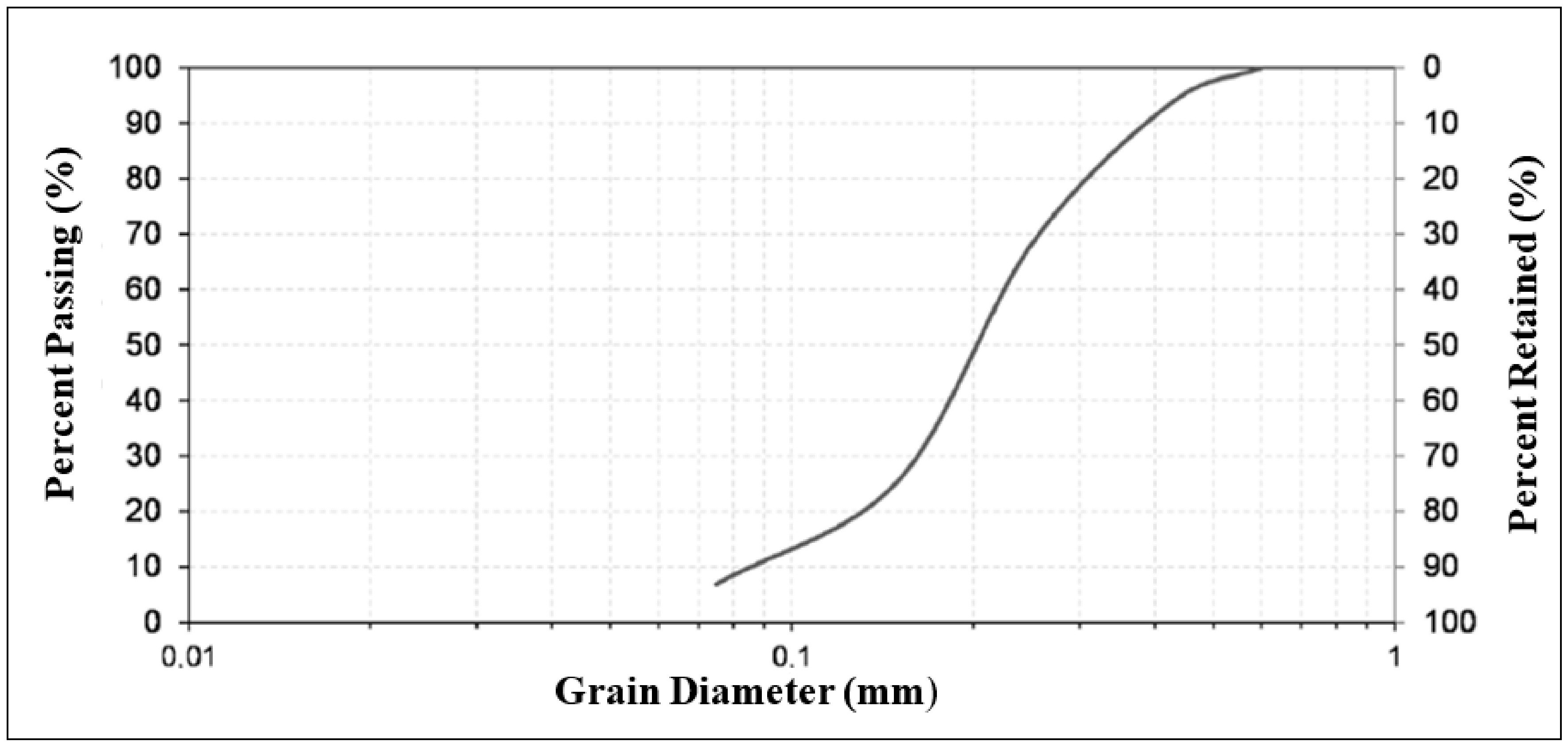
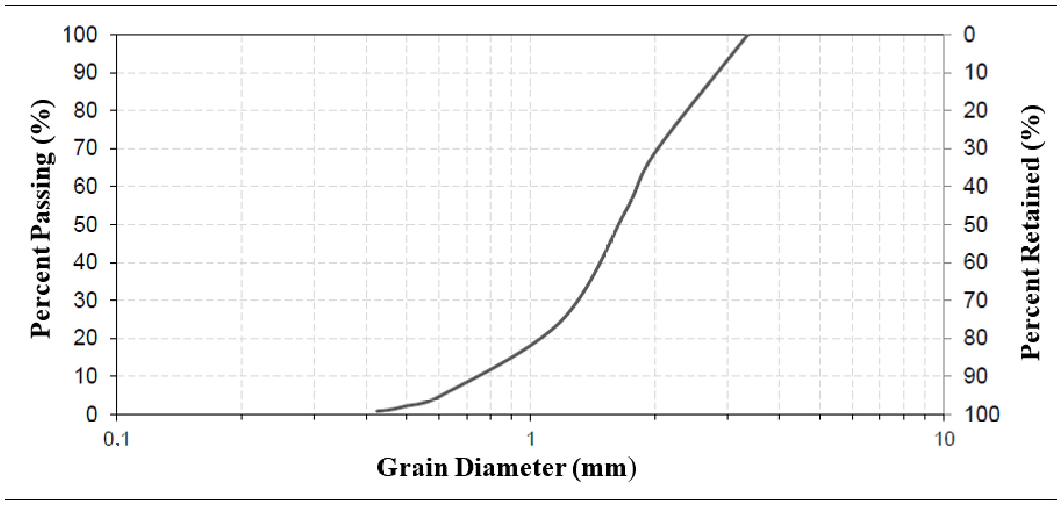
The granulometric curves of the materials used in this study are presented in Figures 3 and 4. Figure 3 shows the grain size distribution of the natural sediment collected from the adduction channel of the Salto Paraopeba Small Hydropower Plant, while Figure 4 presents the granulometric curve of the rubber granulate used as a sediment surrogate in the physical model.

Figure 3
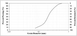
Grain size distribution curve of the sediment sample from the adduction channel of the Salto Paraopeba SHP.

Figure 4
Grain size distribution curve of the rubber granulate used in the physical model.

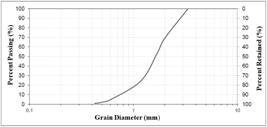
The comparison between both curves indicates that the rubber material exhibits a granulometric distribution compatible with the prototype sediment, particularly in terms of representative grain diameters. This similarity is essential to ensure sedimentological representativeness in reduced-scale physical modeling.

Campello (2017), through an experimental investigation of settling velocity and incipient motion conditions, concluded that ground tire rubber presents satisfactory hydraulic and sedimentological behavior when compared to natural sand. The author demonstrated that the rubber particles adequately reproduce key sediment transport characteristics, supporting their use as a surrogate material in movable-bed physical models.

Thus, based on both the granulometric compatibility and the findings of Campello (2017), the rubber granulate adopted in this study can be considered a suitable representation of the real sediment of the PCH Salto Paraopeba.

The sedimentological similarity of the rubber granulate used in the physical model was investigated by Campello (2017), who studied the physical and hydrodynamic characteristics of ground tire rubber grain as a viable alternative to sand in movable-bed physical models. The author conducted experimental measurements of settling velocity and incipient motion for both rubber and sand particles, concluding that the results were satisfactory for an exploratory analysis of rubber as a sand substitute in terms of settling velocity and onset of motion for use in movable-bed physical models. Specifically, the critical Shields shear stress of the rubber granulate fell within the dispersion range of experimental data reported by Shields and other authors, and the onset of particle motion can be assessed using the Shields curve. Furthermore, the settling velocity of the rubber, once the drag coefficient is corrected for particle shape, can be determined by the equation of Camenen (2007). These findings support the use of rubber granulate as a surrogate sediment material in the present study, acknowledging that residual deviations in density and shape relative to natural sand are inherent limitations of this type of physical model.

After 2.5 hours — which corresponds to the compressed simulation of five prototype years (2013–2017), obtained by applying the time scale factor of 1:2,483 (Table 1) and replacing the full daily-flow hydrograph with the mean flow of the peak-flow waves (Q_MM), as detailed by Teixeira et al. (2020) — the amount of sediment that was retained in the reservoir was measured in each simulation. It is worth noting that the full application of the time scale would imply approximately 17.6 hours of uninterrupted model operation for five prototype years. However, since numerical simulations demonstrated that sediment transport occurred exclusively during peak-flow events — flood waves of approximately 50 days in the first three hydrological years and 30 days in the last two, corresponding to 30 and 20 minutes in the model, respectively — the remaining low-flow periods contribute no sediment movement and need not be reproduced. This approach is consistent with previous findings that sediment transport in the PCH is predominantly associated with peak-flow conditions (Teixeira et al., 2022). Furthermore, preliminary laboratory tests showed that inserting sediment over too short a time interval caused cohesive attractions among rubber particles, hindering their transport; a minimum duration of 30 minutes per year was therefore adopted for all five years, yielding the total of 2.5 hours. Thus, the TE was obtained for each series of simulated flows. The experimental TE values were compared with those calculated using the empirical methods of Brune, Heinemann and Churchill. For this calculation, the five series of flows in Table 3 and geometric data from the small scale model, such as reserve capacity and length of the reservoir, were used.

Table 3
Experimental trap efficiencies observed and those calculated by empirical methods for the five series of flows for the period 2013-2017.

Serie QMM	TE (%)
	Experimental	Brune	Heinemann	Churchill
1ª	99.38	96.01	89.66	47.79
2ª	93.66	95.53	89.05	44.80
3ª	87.84	95.27	88.73	43.26
4ª	88.40	94.34	87.56	38.12
5ª	91.30	96.11	89.79	48.59

Determination of the best empirical method of TE calculation for the small scale model and TE variation due to uncertainties in flow values

In order to determine the best TE calculation method for the PCH small scale model reservoir and to evaluate how much the inaccuracy in the flow values can affect the TE result in the prototype, 1000 synthetic Q_MM series were stochastically generated. These series are for the period 2013-2017 and were generated using the AR(1) model, according to the procedure previously described. From these series, thousands of TE values were calculated for the prototype and thousands more for the small scale model. The three methods consolidated in the literature were used for the calculation - Brune, Heinemann and Churchill, and 1000 TE values were calculated for each method.

With the thousands of TE values, it was possible to compare the calculated ones obtained by the empirical methods with the TE observed in the small scale model. It is noteworthy that the TE in the physical model was found using the historical series of Q_MM for the period 2013-2017, which is the fifth series shown in Table 2. From this comparison, it was possible to observe which is the best method of TE calculation for the small scale model.

The same procedure was performed for the PCH, that is, the 1000 TE values calculated for the prototype were compared with the real TE value. The stochastically generated flow values were also compared with those of the PCH historical series. In this way, the relation between the TE variation due to the flow variation was obtained, in other words, it was obtained how the uncertainties in the flow values can influence in the TE results, when using the empirical methods.

To quantify the agreement between empirically calculated and experimentally observed TE values, three statistical metrics were computed: the Root Mean Square Error (RMSE), which weights larger deviations more heavily and reflects the overall magnitude of the error; the Mean Bias (Bias), which indicates whether a method systematically overestimates or underestimates the observed values; and the Mean Absolute Error (MAE), which expresses the average error directly in percentage points of TE, offering a straightforward measure of accuracy.

RESULTS AND DISCUSSION

Determination of the TE in the small scale physical model

Table 3 shows the experimental TE value observed in the small scale model and those calculated by the three empirical methods: Brune, Heinemann and Churchill. Both experimental and calculated TE’s refer to the five series of flows shown in Table 2.

It is observed in Table 3 that, for the first two series of Q_MM, the empirical method that resulted in a TE value closer to the value of the small scale model was that of Brune. This method was also recognized with results satisfactorily close to what happened in the work carried out by Sultana & Naik (2015), which evaluated the applicability of some empirical methods for the Sriramsagar reservoir, located in South India.

Rabelo et al. (2025), applying the Brune method to estimate sediment retention indices in Brazilian semi-arid reservoirs, also confirmed the method's tendency to slightly overestimate retention values relative to observed sedimentation data, consistent with the positive bias of +3.34% identified in the present study (Table 4).

Table 4
Statistical performance metrics computed between the TE values calculated by each empirical method.

Metrics	Brune	Heinemann	Churchill
RMSE (%)	5.07	4.89	47.73
Bias (%)	3.34	-3.16	-47.60
MAE (%)	4.68	3.51	47.60

In the other series, the experimental TE values are closer to those calculated using the Heinemann method. Issa et al. (2015) also obtained the TE result calculated with this method close to what was observed in the Mosul Dam reservoir. In his study, the calculated value differed from the real by less than 2%. Li et al. (2018) also obtained satisfactory results with the Heinemann method for the prediction of TE.

Based on Table 3, it appears that there was not only one empirical method that provided better TE values for the small scale model. In this present study, the Brune and Heinemann methods were shown more promising. Therefore, it is observed that the result of the empirical method can vary according to the series of flows used, even though they are for the same period (2013-2017) and are generated stochastically following the same mean and standard deviation. Note that the error is always less than 5%, regardless of the method evaluated with the experimental one. This shows that the calculated results are close to those observed, indicating a satisfactory fit of these models with the reservoir in this paper.

The Heinemann method yielded the lowest RMSE (4.89%) and MAE (3.51%), with a Bias of −3.16%, indicating a marginal tendency toward underestimation with no significant systematic deviation. The Brune method presented a positive Bias of +3.34%, corroborating its well-documented tendency to overestimate TE values (Costa, 2012). The Churchill method exhibited substantially larger errors than the other two methods, with an RMSE of 47.73% and a Bias of −47.60%, demonstrating its inadequacy for the hydraulic and sedimentological conditions of the reservoir examined in this study. The results are summarized in Table 4.

Of the three empirical methods evaluated, the one with the worst result was that of Churchill. Lewis et al. (2013) analyzed the difference in TE in temperate and tropical countries, focusing on the irregularity of sediment flow that occurs in tropical countries, while in temperate countries there is a more constant sediment disposal. The Churchill method relies on the Sedimentation Index. The correct application of this index requires a discharge representative of the full hydrological period — typically a long-term mean annual flow. In this study, however, the input discharge used was the average flow of the maximum-period waves (Q_MM), which correspond to flood pulses lasting approximately 50 days per year at the PCH. These high-flow events yield a Q_MM substantially higher than the long-term annual mean, which reduces the computed SI and consequently underestimates the TE predicted by Churchill's method. This mismatch between the discharge type required by the method and the discharge available from the physical model experiments constitutes the primary reason for the poor fit of the Churchill method observed in this study. Thus, this explains the worst result obtained for TE value calculated using the method proposed by Churchill.

Determination of the best empirical method for calculating TE for the small scale model and TE variation due to uncertainty in flow values

The flow values have inaccuracies, since the methods used in their measurements have uncertainties. It so happens that the flow is one of the input parameters of the empirical methods for calculating the TE. It is noteworthy that in some methods the input parameter is the volume affluent to the reservoir, which is related to the flow. Thus, using stochastic modeling for the generation of synthetic series of flows, the best TE calculation method was determined for the PCH small scale physical model and the influence that uncertainty in the flow value can have on the values of TE calculated by the methods of Brune, Heinemann and Churchill were verified.

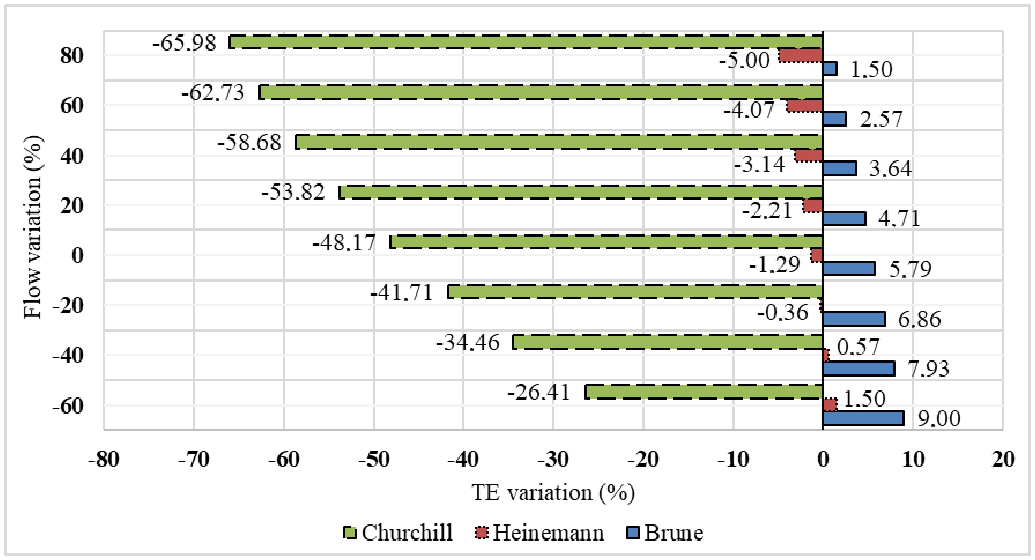
In order to determine the best empirical TE method for the small scale model, the TE was calculated by each of the three methods, using the 1000 stochastic generated synthetic Q_MM series for the period 2013-2017. The thousands of TE calculated were compared with the TE observed in the small scale model, which was 91.3%. It is worth mentioning that the base experimental TE value refers to the historical series of Q_MM in the period 2013-2017. In Figure 5, it is possible to observe the variation of the difference between the calculated and the experimental TE value versus the variation of the difference between the synthetic flows generated stochastically and those of the historical series, in the period 2013-2017.

Figure 5
TE variation as a function of flow variation, for the small scale model.

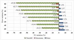
Additionally, Figure 5 allows a clearer interpretation of the comparative performance of the empirical methods: for all flow variation ranges analyzed, the Heinemann method consistently presented the smallest deviation relative to the experimental TE value. For example, when the flow variation was 0%, the error associated with the Heinemann method was −1.29%, whereas the Brune and Churchill methods presented deviations of +5.79% and −48.17%, respectively. This pattern is maintained across the entire variation range, indicating greater robustness and stability of the Heinemann method in relation to flow uncertainties.

The TE variation (Y-axis) represents the difference between the TE calculated with each stochastically generated flow and the experimentally observed TE of 91.3% (obtained in the physical model and confirmed equivalent to the prototype by Teixeira et al., 2020). The wide flow variation range (−60% to +80%) results from the stochastic generation process: each of the 1000 generated flows minus the observed historical mean yields differences spanning this range. This behavior is inherent to stochastic simulations of hydrological series and reflects the natural variability of flow regimes, rather than deficiencies in model performance (Teixeira et al., 2022). This does not indicate poor model fit — the stochastically generated series still adjusts well to the PCH data overall, even though individual draws can deviate substantially from the mean. The flow variation range (−60% to +80%) represents the dispersion observed in the stochastically generated series relative to the historical data. However, this range should be interpreted as a modeling outcome rather than a direct representation of measurement uncertainty.

In Figure 5, it can be seen that when the synthetic series of flows had values ​​close to the historical series, that is, the flow variation was close to 0%, the Heinemann method showed a TE variation close to 0%. Therefore, the best method to calculate the TE of the small scale model of the PCH was that of Heinemann. Issa et al. (2015) also concluded that Heinemann presented good results for estimating the TE of the Mosul Dam reservoir, located in the Iraq region, which has a tropical climate. As concluded by Revel et al. (2015), when looking at Figure 5, it is clear that the Brune model has a built-in tendency to overestimate the TE values, given that even when there is no variation in the flow, that is, the flow value is approaching the historical series, the TE results by Brune are already overestimated by 10%. Garg et al. (2020) also found that Brune's empirical method overestimated the TE value and was not appropriate for the Tehri reservoir in India.

As discussed above, from Table 3, for the five simulations performed in the small scale model, in two of them the TE values calculated by the Brune method were closer to what was observed experimentally, while in the other cases the Heinemann method showed better results. In other words, based only on the experimental results, it was not possible to state which is the best empirical method to calculate the TE. However, when analyzing the TE variation with the flow variation, something possible due to the stochastic flow generation, it was possible to conclude that the best method to calculate the TE for the PCH small scale model was Heinemann's. Thus, it is suggested that in future reservoir projects, before adopting an empirical method to calculate the TE, stochastic modeling of flows should be carried out and the best method selected based on this simulation, as done in this present study.

From Figure 5, it can be noticed that if the flow has an error of approximately 80%, in the methods of Brune and Heinemann, this error causes a variation in the TE value of less than 10%. The TE values calculated by Brune's method tend to be 6% higher than those by Heinemann, regardless of the flow variation value. This observed result is aligned with what was expected, since, as stated by Costa (2012), the TE values calculated using Brune's method tend to be 4 to 10% higher than those calculated with Heinemann's.

While Brune and Heinemann's methods present little TE variation, even for large flow variations, Churchill's method presents great TE variation, which is almost 70%, when the flow varies by approximately 80%. Thus, it is observed that Churchill's method did not fit well with the small scale model. It is observed that the error is already implicit in its use because even when there is no variation in the flow, this method showed a divergence of 50% in TE. Previously, when comparing the results of the experimental TE's of the small scale model with those calculated by Churchill's method (Table 3), the differences between them had been greater than those of the other methods.

According to Carvalho et al. (2000) the Churchill method is indicated for small reservoirs, which have a reserve volume smaller than 10hm³, which is the case of the reservoir in this study. However, Borland (1971) apud Verstraeten & Poesen (2000) when comparing the methods of Brune and Churchill using the John Martin Reservoir, located in Colorado (USA), with 744.405 hm³ of capacity (Bern et al., 2020), obtained a good result with the method of Churchill. This shows that the TE results calculated with this method are influenced not only by the reservoir size but also by characteristics inherent to the sediment, given that the Churchill curve distinguishes between locally produced sediments and those that come from upstream reservoirs, the latter being of finer granulometry.

Churchill is the only one among the three methods discussed that considers the Sedimentation Index (SI) of the reservoir, which in turn will be influenced by the retention time of the water inside the reservoir and the average flow velocity. Garg et al. (2020) cited the intrinsic complexity of the SI, used in the Churchill method. In tropical countries, it is not feasible to approximate an average flow, which can occur in other locations. Thus, the TE value calculated with the Churchill method results in different values depending on the particularities of the reservoir to which it is applied, and may return values that are very different from those expected, as is the case for the reservoir in this paper.

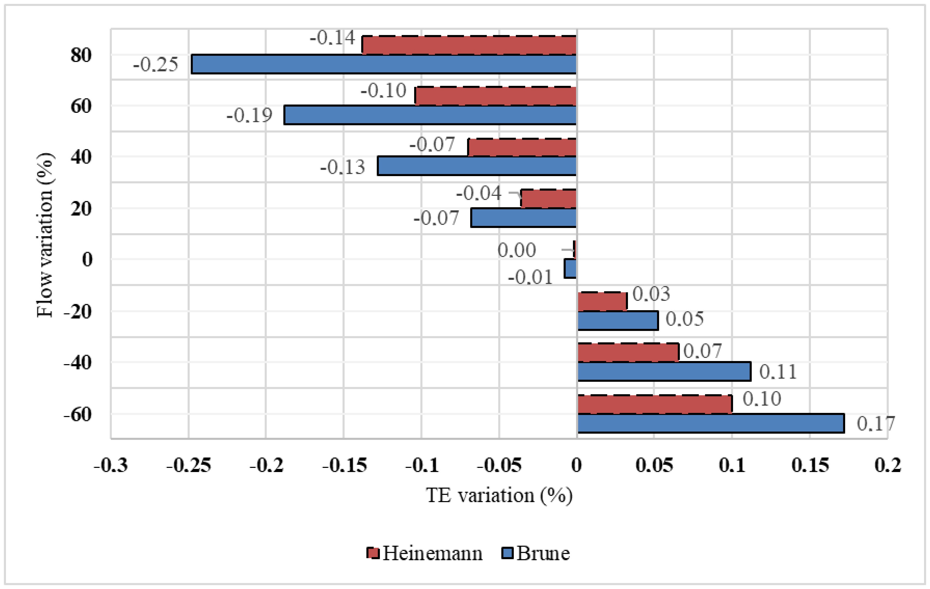
As the Churchill method did not show satisfactory results, the influence of the uncertainties of the flow values in the TE calculation was analyzed using only the Brune and Heinemann methods, as shown in Figure 6.

Figure 6
TE variation as a function of flow variation for the prototype.

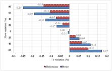
When analyzing the reservoir in the real scale, that of the prototype, in Figure 6, small variations in the TE values ​​can be observed as a result of variations in flow rates, which are below 1%. This relatively low sensitivity of TE to flow variations is consistent with findings from numerical sediment transport modeling in Brazilian rivers. Marciano et al. (2024) reported that sediment retention at a river confluence in Minas Gerais was approximately 50% during an extreme flood event, suggesting that geometric and structural characteristics of the hydraulic system may exert a more decisive influence on retention efficiency than flow variability alone.

That is, as much as there are uncertainties in the flow values, which, for example, can be caused by the measurement methods, these uncertainties had little effect on the empirical methods of Brune and Heinemann in calculating the TE. Thus, in the design process of Reservoirs, it has to be evaluated which is the best empirical method, as it will be the one that will most influence the TE result, and its input parameters, such as flow, tend to have less influence. However, one of the reasons that may have resulted in a small interference of the flows in the TE values ​​is the fact that the reservoir used in this work is small so that for larger reservoirs the influence of the flow in the TE calculation could be more significant. In addition, the period studied (2013-2017) was one of small flows, due to the long period of drought in the PCH region. This represents a limitation of the study, as sediment inflow is significantly higher during wetter periods, and the empirical methods may respond differently under higher-flow conditions. Thus, even in small reservoirs, such as the PCH, but in periods of higher inflows, maybe they can interfere more in the TE estimation when using empirical methods.

The results obtained in this study are specific to the PCH Salto Paraopeba small hydropower plant reservoir and its reduced-scale physical model, and caution is required when extrapolating them to other reservoirs. The physical model was designed to represent a small reservoir (volume of 0.711 hm³ in the prototype) with a particular geometry, flow regime, and sediment transport regime. As discussed in Section 2.4, the sediment surrogate used — rubber granulate with ρs = 1,130 kg/m³ and d50 = 1.7 mm — was chosen to satisfy sedimentological similarity criteria within the constraints of the physical model, but differs substantially from natural sediment in absolute density and grain size. The empirical methods of Brune, Heinemann, and Churchill were calibrated using data from reservoirs with natural sediments and varying geometric and hydrological characteristics. Therefore, the identification of Heinemann's method as the best-fitting approach for this specific reservoir and sediment surrogate does not necessarily hold for reservoirs with different capacity-to-inflow ratios, sediment grain size distributions, or flow regimes. Future studies should replicate this stochastic-physical modeling approach using natural sediment or other surrogate materials across a broader range of reservoir types to assess the generalizability of these findings.

CONCLUSION

From the comparison of empirical methods, the stochastic generation of flow values, and the influence of inaccuracy in the value of this parameter, it is concluded:

• The methods of Brune and Heinemann were the ones that presented TE results closer to those observed in the small scale model. However, only based on the experimental data it was not possible to establish which method best fit the model, because while Brune was the best for two series of simulated flows, Heinemann presented the best result for three series. Thus, the result of the empirical method can vary according to the series of flows used, even if they are from the same period;

• By stochastically generating 1000 synthetic series of flows for the small scale model and, through them, calculating the TE, using the three empirical methods, it was observed that the Heinemann method presented better results. In other words, it was the method that presented TE values closer to those observed in the small scale model. Therefore, as in the literature there are several methods to calculate the TE of reservoirs, and finding the one that best suits each reservoir is not trivial, it is suggested that in future reservoir projects stochastic modeling of flows be carried out to assist in choosing the best method for calculating TE for that reservoir;

• Churchill's method was the one that showed the worst results, both in the experimental analysis and in the stochastic analysis;

• For the prototype, when evaluating the influence of flow variation on TE results, it is clear that, as much as there are uncertainties in flow values, which can be caused, for example, by measurement methods, these variations did not affect the value of TE in a significant manner. However, it is noteworthy that the PCH reservoir is small and the simulated flows were small, so that larger reservoirs and larger flows can cause the TE results to be more affected by uncertainties in flow values.

DATA AVAILABILITY STATEMENT

Research data is available in the body of the article.

REFERENCES

• Alighalehbabakhani, F., Miller, C. J., Selegean, J. P., Barkach, J., Mohsen, S., Abkenar, S., Dahl, T., & Baskaran, M. (2017). Estimates of sediment trapping rates for two reservoirs in the Lake Erie watershed: past and present scenarios. Journal of Hydrology, 544, 147-155. https://doi.org/10.1016/j.jhydrol.2016.11.032
  » https://doi.org/10.1016/j.jhydrol.2016.11.032
• Araújo, P., Rodrigues, S. O. A., Costa, V. S. C., & Avelar, A. S. (2017). Análise do comportamento hidrológico da bacia Córrego Sujo, Teresópolis (RJ). Os Desafios da Geografia Física na Fronteira do Conhecimento, 1, 739-752. https://doi.org/10.20396/sbgfa.v1i2017.1844
  » https://doi.org/10.20396/sbgfa.v1i2017.1844
• Borland, W. M. (1971). Reservoir sedimentation. In H. W. Shen (Ed.), River mechanics (Vol. 2, pp. 29.1-29.38). Fort Collins, CO: Colorado State University.
• Bern, C. R., Holmberg, M. J., & Kisfalusi, Z. D. (2020). Effects of John Martin Reservoir, Colorado on water quality and quantity: assessment by chemical, isotopic, and mass-balance methods. Journal of Hydrology X, 7, 100051. https://doi.org/10.1016/j.hydroa.2020.100051
  » https://doi.org/10.1016/j.hydroa.2020.100051
• Brune, G. M. (1953). Trap efficiency of reservoirs. Transactions - American Geophysical Union, 34(3), 407-418. https://doi.org/10.1029/TR034i003p00407
  » https://doi.org/10.1029/TR034i003p00407
• Camenen, B. (2007). Simple and general formula for the settling velocity of particles. Journal of Hydraulic Engineering, 133(2), 229-233. https://doi.org/10.1061/(ASCE)0733-9429(2007)133:2(229)
  » https://doi.org/10.1061/(ASCE)0733-9429(2007)133:2(229)
• Campello, B. S. C. (2017). Estudo da velocidade de queda e do início do movimento das partículas de borracha e areia (Dissertação de mestrado). Universidade Federal de Minas Gerais, Belo Horizonte.
• Carvalho, L. S., Saliba, A. P. M., Santos, R. S. F., Haselbauer, M., Velasco, D., Viana, E. M. F., Martinez, C. B., Costa, M. E. F., & Freitas, F. L. (2014). Desenvolvimento do projeto do modelo reduzido da PCH Salto do Paraopeba. In XXVI Congresso Latinoamericano de Hidráulica, Santiago, Chile. Madrid: IAHR.
• Carvalho, N. O. (2008). Hidrossedimentologia prática (2. ed.). Rio de Janeiro: Editora Interciência.
• Carvalho, N. O., Filizola Júnior, N. P., Santos, P. M. C., & Lima, J. E. F. W. (2000). Guia de avaliação de assoreamento em reservatórios Brasília: Agência Nacional de Energia Elétrica.
• Churchill, M. A. (1948). Discussion of analysis and use of reservoir sedimentation data. In Proceedings of the Federal Interagency Sedimentation Conference: Bureau of Reclamation (pp. 139-140). Washington, DC: US Department of the Interior.
• Costa L. F. (2012). Análise de sensibilidade dos parâmetros utilizados na determinação de taxas de assoreamento de reservatórios (Tese de doutorado). Universidade Federal do Rio de Janeiro, Rio de Janeiro.
• Coz, J. L., Camenen, B., Peyrard, X., & Dramais, G. (2012). Uncertainty in open-channel discharges measured with the velocity–area method. Flow Measurement and Instrumentation, 46, 193-194. https://doi.org/10.1016/j.flowmeasinst.2014.07.004
  » https://doi.org/10.1016/j.flowmeasinst.2014.07.004
• Garg, A. A., Alemayehu, A. S., & Sumedha, C. (2020). Assessment of sedimentation and useful life of Tehri reservoir using integrated approaches of hydrodynamic modelling, satellite remote sensing and empirical curves. Current Science, 118(3), 411-420. https://doi.org/10.18520/cs/v118/i3/411-420
  » https://doi.org/10.18520/cs/v118/i3/411-420
• Guo, A., Chang, J., Wang, Y., Huang, Q., & Zhou, S. (2018). Flood risk analysis for flood control and sediment transportation in sandy regions: A case study in the Loess Plateau, China. Journal of Hydrology, 560, 39-55. https://doi.org/10.1016/j.jhydrol.2018.02.076
  » https://doi.org/10.1016/j.jhydrol.2018.02.076
• Hager, W. H. (2018). Bed-load transport: advances up to 1945 and outlook into the future. Journal of Hydraulic Research, 56(5), 596-607. https://doi.org/10.1080/00221686.2017.1405370
  » https://doi.org/10.1080/00221686.2017.1405370
• Heinemarm, H. G. (1981). A new sediment trap efficiency curve for small reservoirs. Journal of the American Water Resources Association, 17(5), 825-830. https://doi.org/10.1111/j.1752-1688.1981.tb01304.x
  » https://doi.org/10.1111/j.1752-1688.1981.tb01304.x
• Issa, E., Al-Ansari, N., Knutsson, S., & Sherwani, G. (2015). Monitoring and evaluating the sedimentation process in mosul dam reservoir using trap efficiency approaches. Engeneering, 7, 190-202. https://doi.org/10.4236/eng.2015.74015
  » https://doi.org/10.4236/eng.2015.74015
• Lewis, S. E., Bainbridge, Z. T., Kuhnert, P. M., Sherman, B. S., Henderson, B., Dougall, C., Cooper, M., & Brodie, J. E. (2013). Calculating sediment trapping efficiencies for reservoirs in tropical settings: A case study from the Burdekin Falls Dam, NE Australia. Water Resources Research, 49(2), 1017-1029. https://doi.org/10.1002/wrcr.20117
  » https://doi.org/10.1002/wrcr.20117
• Li, J., Li, W., Yang, W., Mu, L., Jin, Z., & Zhang, D. (2018). Estimating the sediment trap efficiency and lifespan of cascaded reservoirs in the Upper Yangtze River Basin, China. Lakes and Reservoirs: Research and Management, 23(3), 204-216. https://doi.org/10.1111/lre.12232
  » https://doi.org/10.1111/lre.12232
• Maldonado, L. H., Wendland, E. C., & Porto, R. D. M. (2015). Avaliação de métodos de baixo custo para medição de vazão em córregos. Revista Ambiente & Água, 10(2), 402-412. https://doi.org/10.4136/ambi-agua.1293
  » https://doi.org/10.4136/ambi-agua.1293
• Marciano, A. G., Assireu, A. T., Azevedo, S. C., Silva, B. C., Abreu, A. T., & Nalini Júnior, H. A. (2024). Dramatic changes in the confluence morphology drived by an extreme hydrologic pulse: impacts to River Doce restoration. RBRH, 29, e9. https://doi.org/10.1590/2318-0331.292420230139
  » https://doi.org/10.1590/2318-0331.292420230139
• Morris, G. L. (2020). Classification of management alternatives to combat reservoir sedimentation. Water, 12(3), 861. https://doi.org/10.3390/w12030861
  » https://doi.org/10.3390/w12030861
• Mulu, A., & Dwarakish, G. S. (2015). Different approach for using trap efficiency for estimation of reservoir sedimentation. An overview. Aquatic Procedia, 4, 847-852. https://doi.org/10.1016/j.aqpro.2015.02.106
  » https://doi.org/10.1016/j.aqpro.2015.02.106
• Obreja, F. (2012). Assessment of trap efficiency of the reservoirs in the Siret Basin (Romania). Scientific Annals of Stefan Cel Mare University of Suceava, 21(1), 107-117. https://doi.org/10.4316/GEOREVIEW.2012.21.1.60
  » https://doi.org/10.4316/GEOREVIEW.2012.21.1.60
• Oliveira, J. F. D., Coelho, G., & Carvalho, R. N. (2024). Determination of suspended sediment rating curve and models to estimate the suspended solids concentration in the Pandeiros river, Brazil. RBRH, 29, e16. https://doi.org/10.1590/2318-0331.292420230138
  » https://doi.org/10.1590/2318-0331.292420230138
• Rabelo, D. R., Araújo, J. C., & Cavalcante, A. A. (2025). Impacts of erosion and sedimentation on reservoirs in the Seridó river basin: a hydrosedimentological assessment in the Brazilian semiarid region. RBRH, 30, e32. https://doi.org/10.1590/2318-0331.302520250001
  » https://doi.org/10.1590/2318-0331.302520250001
• Revel, N. M. T. K., Ranasiri, L. P. G. R., Rathnayake, R. M. C. R. K., & Pathirana, K. P. P. (2015). Estimation of sediment trap efficiency in reservoirs - An experimental study. Engineer, 48(2), 43-49. https://doi.org/10.4038/engineer.v48i2.6833
  » https://doi.org/10.4038/engineer.v48i2.6833
• Santos, E. S., & Cunha, A. C. (2015). Análise de cenários hidrossedimentométricos para estimar taxas de assoreamento e vida útil da UHE Cachoeira Caldeirão no Rio Araguari/AP-Brasil. Biota Amazônia, 5(3), 88-97. https://doi.org/10.18561/2179-5746/biotaamazonia.v5n3p88-97
  » https://doi.org/10.18561/2179-5746/biotaamazonia.v5n3p88-97
• Schleiss, A. J., Franca, M. J., Juez, C., & Cesare, G. (2016). Reservoir sedimentation. Journal of Hydraulic Research, 54(6), 595-614. https://doi.org/10.1080/00221686.2016.1225320
  » https://doi.org/10.1080/00221686.2016.1225320
• Shrestha, B., Cochrane, T. A., Caruso, B. S., Arias, M. E., & Piman, T. (2016). Uncertainty in flow and sediment projections due to future climate scenarios for the 3S Rivers in the Mekong Basin. Journal of Hydrology, 540, 1088-1104. https://doi.org/10.1016/j.jhydrol.2016.07.019
  » https://doi.org/10.1016/j.jhydrol.2016.07.019
• Sultana, Q., & Naik, M. G. (2015). Estimation of trap efficiency of Sriramsagar reservoir. International Journal of Research in Engineering and Technology, 4(23), 116-122. https://doi.org/10.15623/ijret.2015.0423020
  » https://doi.org/10.15623/ijret.2015.0423020
• Tan, G., Chen, P., Deng, J., Xu, Q., Tang, R., Feng, Z., & Yi, R. (2019). Review and improvement of conventional models for reservoir sediment trapping efficiency. Heliyon, 5(9), e02458. https://doi.org/10.1016/j.heliyon.2019.e02458
  » https://doi.org/10.1016/j.heliyon.2019.e02458
• Teixeira, E. K. C. (2019). Simulação estocástica do assoreamento em reservatórios (Tese de doutorado). Universidade Federal de Minas Gerais, Belo Horizonte.
• Teixeira, E. K. C., Rinco, A. V., Coelho, M. M. L. P., Saliba, A. P. M., Pinto, E. J. A., & Furtado, L. M. (2020). Methodology for physical modeling of reservoir sedimentation. RBRH, 25(27), e27. https://doi.org/10.1590/2318-0331.252020190093
  » https://doi.org/10.1590/2318-0331.252020190093
• Teixeira, E. K. C., Coelho, M. M. L. P., Pinto, E. J. A., Rinco, A. V., & Saliba, A. P. M. (2022). Stochastic simulation in reservoir sedimentation estimation: application in a PCH. Anais da Academia Brasileira de Ciências, 94(Suppl. 3), e20211573. https://doi.org/10.1590/0001-3765202220211573
  » https://doi.org/10.1590/0001-3765202220211573
• Valent, P., Výleta, R., & Danácová, M. (2019). A joint sedimentation-flood retention assessment of a small water reservoir in Slovakia: a new hope for old reservoirs? Geosciences, 9(4), 158. https://doi.org/10.3390/geosciences9040158
  » https://doi.org/10.3390/geosciences9040158
• Van Rijn, L. C. (2013). Sedimentation of sand and mud in reservoirs in rivers Recuperado em 4 de novembro de 2020, de https://www.leovanrijn-sediment.com
  » https://www.leovanrijn-sediment.com
• Verstraeten, G., & Poesen, J. (2000). Estimating trap efficiency of small reservoirs and ponds: methods and implications for the assessment of sediment yield. Progress in Physical Geography, 24(2), 219-251. https://doi.org/10.1177/030913330002400204
  » https://doi.org/10.1177/030913330002400204

Edited by

• Editor-in-Chief:
  Adilson Pinheiro

• Associated Editor:
  Fernando Mainardi Fan

Publication Dates

• Publication in this collection
  20 July 2026
• Date of issue
  2026

History

• Received
  16 Dec 2025
• Reviewed
  06 Apr 2026
• Accepted
  04 May 2026