Simulation of aquifers under steady-state conditions using the Multi-Point Flux Approximation with Diamond Stencil (MPFA-D) method

Simulação de aquíferos em condições de regime permanente utilizando o método de Aproximação de Fluxo por Múltiplos Pontos com estêncil diamante (MPFA-D)

ABSTRACT

The simulation of groundwater flow in complex porous media requires sophisticated numerical methods capable of handling general geometries, strongly discontinuous and anisotropic coefficients, and ensuring local mass conservation. In this sense, we use for the first time, a finite volume method of the type MPFA-D (Multi-Point Flux Approximation with Diamond Stencil), for the approximation of the hydraulic head equation in aquifers. To test the accuracy and robustness of the method, we solved problems related to the simulation of aquifers and compared them with analytical solutions and results from the MODFLOW 6 simulator.

Keywords:
Groundwater simulation; MPFA-D method; Hydraulic head equation; Steady-state aquifers; MODFLOW 6

RESUMO

A simulação do fluxo de águas subterrâneas em meios porosos complexos requer métodos numéricos sofisticados, capazes de lidar com geometrias gerais, coeficientes fortemente descontínuos e anisotrópicos, e garantir a conservação da massa local. Nesse sentido, utilizamos, pela primeira vez, um método de volumes finitos do tipo MPFA-D (Multi-Point Flux Approximation with Diamond Stencil) para a aproximação da equação de carga hidráulica em aquíferos. Para testar a precisão e a robustez do método, resolvemos problemas relacionados à simulação de aquíferos e os comparamos com soluções analíticas e resultados do simulador MODFLOW 6.

Palavras-chave:
Simulação de águas subterrâneas; Método MPFA-D; Equação da carga hidráulica; Aquíferos no estado estacionário; MODFLOW 6

INTRODUCTION

The largest aquifers in the world are located in South America, and Brazil has significant groundwater resources that are essential for human consumption, agriculture, and livestock farming, especially in arid regions (Instituto Trata Brasil, 2023). This resource is extracted through pumping wells, the number of which exceeded 2.5 million in 2019, most of which are clandestine: about 88%, i.e. about 2.2 million wells without official registration. Ineffective management, indiscriminate exploitation and lack of proper regulation can lead to overexploitation, degradation and pollution of these sources and have a negative impact on the environment and public health (Muyinda et al., 2014; Bakker & Post, 2022). To mitigate these impacts, technological tools are widely used, such as commercial simulators based on numerical methods and capable of analyzing the dynamics of groundwater flow (Maus, 2011). In this context, the improvement or development of new technologies based on sophisticated numerical methods is crucial, provided they can deal with complex geologies and provide more accurate and reliable results. The classical numerical methods currently used in commercial simulators include: the finite element method (FE) used in the FEFLOW simulator, the finite difference method (FD) used in the MODFLOW 6 simulator and the finite volume (FV) method used in ANSYS Fluent. The FD method is a widely used approach in aquifer modeling due to its simplicity and computational efficiency (Muyinda et al., 2014). FE method offers greater flexibility in the treatment of complex geometries, while FV method is characterized by its accuracy in the local conservation of physical properties, which enables effective simulations in complex porous media (Bertolazzi & Manzini, 2004; Blazek, 2015; Maliska, 2004). In recent decades, the numerical formulation of flows in porous media has been the subject of intensive studies, which have made significant contributions both in theory and in practical application. To overcome the limitations of traditional finite difference methods, Aavatsmark et al. (1996) and later Aavatsmark (2002) introduced the Multi-Point Flux Approximation with O-shaped stencil (MPFA-O), a method specifically designed to solve the pressure equation in anisotropic porous media using non-orthogonal quadrilateral grids. Over time, the MPFA framework has been extended, leading to several variants, including the MPFA-L method proposed by Aavatsmark (2002). MPFA-TPS (Edwards & Zheng, 2008), MPFA-Enriched (Chen et al., 2008; Pal et al., 2006), as well as methods, such as MPFA-FPS (Edwards & Zheng, 2008; Friis & Edwards, 2011), these methods have not yet been used in the context of groundwater simulation. The methods of the MPFA family (O, L, TPS, FPS) provide very accurate results in highly anisotropic porous media and at the same time cope with distorted polygonal meshes. However, the interpolation of auxiliary variables requires the solution of a system of local linear equations. This implicit interpolation process can lead to additional computational costs, for example, in the simulation of pollutant transport. Klausen et al. (2008), inspired by the FE method, investigated the convergence of MPFA methods in triangular grids applied to the Richards equation and proved their accuracy and stability in groundwater flow simulations. Li et al. (2010) used the FD method centered on a nineteen-point cell to model the three-dimensional groundwater flow at steady state, considering anisotropic and heterogeneous hydraulic conductivity tensors. On the other hand, Gao & Wu (2010) proposed a new FV method of type MPFA-D (Multi-Point Flux Approximation with Stencil Diamond) to solve the diffusion equation in different types of meshes. This method is able to preserve the linearity and maintain the second-order accuracy in very heterogeneous and anisotropic media. Igboekwe & Achi (2011) applied the FD method to approximate the steady state hydraulic head equation without recharge to obtain water flow directions and flow rate. Younes et al. (2013) analyzed the monotonicity of MPFA in highly heterogeneous media and triangular networks and proposed conditions to ensure the positivity of flows by upwind weighting techniques. On the other hand, Suk et al. (2020) modeled groundwater flow using the conservative Galerkin FE method with the aim of increasing accuracy and ensuring local and global conservation. Based on Gao & Wu (2010) and Contreras et al. (2016, 2021), Cavalcante et al. (2020) formulated a three-dimensional extension of the MPFA-D to simulate the two-phase flow of oil and water in fractured reservoirs, taking into account the numerical criteria established by these authors. Aharmouch et al. (2020) used a conservative cell-centered FD method to model saltwater intrusion in coastal aquifers, solving the nonlinear equations by a fully implicit approach using the Newton method coupled to BiCGSTAB. Gao et al. (2021) applied the MPFA-O coupled with a high-order TVD method to solve the pollutant transport equation in polygonal meshes, minimizing numerical dispersion and ensuring mass conservation. Gao et al. (2022) proposed an improved version of MPFA-O to solve the hydraulic head equation in confined and unconfined aquifers by applying it to truly polygonal meshes and obtained good results, even in pathological cases. Farmani et al. (2023) used the FE method with spherical Hankel shape functions to model the percolation of water flow, aiming for greater accuracy and numerical stability, even with few cells. Qian et al. (2023) proposed a vertex-centered MPFA method to simulate the hydraulic head equation in nonconforming meshes and optimize the resolution in regions of interest, such as wells, with low computational cost. Contreras et al. (2023) applied a nonlinear FV method to simulate contaminant transport in groundwater, considering strongly anisotropic molecular diffusion and permeability tensors.

In this paper, for the first time, the hydraulic head equation in complex aquifers is solved by applying the MPFA-D method. This method was originally formulated by Gao & Wu (2010) to solve diffusion problems and later applied to the simulation of oil reservoirs (Contreras et al., 2016, 2019; Cavalcante et al., 2020). According to Contreras et al., (2019). The choice of the MPFA-D method is therefore due to its ability to efficiently handle very heterogeneous and anisotropic porous media and to deal with polygonal distorted meshes, to ensure the local conservation of physical properties and to improve the accuracy of the simulated flows. In addition, the interpolation of auxiliary variables follows an explicit procedure and preserves linearity.

This paper is organized as follows: Section 1 introduces the problem, its relevance and the aims of the study. Section 2 describes the governing equations as well as the initial and boundary conditions. Section 3 explains the formulation of the method used to discretize the equations. Section 4 analyzes different problems to verify the accuracy and robustness of the method. Finally, Section 5 presents the conclusions obtained from the results obtained with the proposed numerical method.

MATERIAL AND METHODS

Mathematical model

We have made some simplifying assumptions for modeling the groundwater flow: We have assumed that the aquifer is horizontal, so that fluctuations in the depth of the porous medium can be neglected. We also assumed that both the fluid and the porous medium are incompressible, so that the fluid density and the porosity of the medium remain constant over time. From these assumptions, Darcy's law and the law of conservation of mass, the authors (Freeze & Cherry, 1979; Fetter, 2018; Langevin et al., 2021; Zhang et al., 2022; Qian et al., 2023) derive the equation of hydraulic head, which is as follows:

$$\nabla \cdot \left(-K\nabla h\right)=f(x,y),K=M{K}_s$$ (1)

Here, h denotes the hydraulic head, K the transmissibility, and $K_s$corresponds to the hydraulic conductivity tensor that fulfills the ellipticity condition, as discussed by Contreras et al. (2019). In addition, M refers to the thickness of the aquifer and f is a term that can include sinks, precipitation, evaporation, or recharge (Zhang et al., 2022; Qian et al., 2023). In unconfined aquifers, the transmissibility can vary spatially and temporally due to the dependence on the hydraulic head, i.e.$K=h{K}_s$.

According to Qian et al. (2023), the problem described by Equation (1) is fully determined if we specify a set of boundary conditions:

$$h(x,t)=h_D,em{\Gamma }_D\times [0,t]$$ (2)

$$-K\nabla h\cdot n=g_N,em{\Gamma }_N\times [0,t]$$ (3)

In this context, ${\Gamma }_D$ and ${\Gamma }_N$ are the Dirichlet and Neumann contours respectively. The scalar function $h_D$ is the hydraulic head known on the Dirichlet contour ${\Gamma }_D$. The flux $g_N$is prescribed on the Neumann contour ${\Gamma }_N$, where $n$ is the unit normal vector pointing outwards from the domain.

NUMERICAL FORMULATION

In this section, the numerical discretization of Equation (1) using the finite volume (FV) method is presented; the MPFA-D method is used for the Darcy flow approximation. Therefore, integrating the Equation (1) in the domain $\Omega$, obtain:

$${\displaystyle \underset{\Omega }{\int }\nabla \cdot vdV=}{\displaystyle \underset{\Omega }{\int }f(x,y)dV},v=-K\nabla h$$ (4)

here $\Omega$ is the continuous domain and V is the infinitesimal volume and $v$ is the Darcy’s velocity. In Equation (4), using the divergence theorem and mean value theorem, we have:

$$\begin{array}{l}{\displaystyle \underset{\Omega }{\int }\nabla \cdot vdV}={\displaystyle \sum _k{\displaystyle \underset{{\Omega }_k}{\int }\nabla \cdot vdV}}={\displaystyle \sum _k{\displaystyle \underset{\partial {\Omega }_k}{\int }v\cdot n_{k}dA}},{\displaystyle \underset{\Omega }{\int }f(x,y)dV}=\\ {\displaystyle \sum _k{\displaystyle \underset{{\Omega }_k}{\int }f(x,y)dV},}{f}_k=\frac{1}{V_k}{\displaystyle \underset{{\Omega }_k}{\int }f(x,y)dV}\end{array}$$ (5)

where ${\Omega }_k$ is the k-th control volume, cell or element of the computational mesh. The surface integral in Equation (5) is approximated using the mean value theorem for integrals. So we have:

$${\displaystyle \underset{\partial {\Omega }_k}{\int }v\cdot n_{k}dA}={\displaystyle \sum _{e\in \partial {\Omega }_k}{v}_e\cdot N_e,}{v}_e=\frac{1}{\left|e\right|}{\displaystyle \underset{\partial {\Omega }_k}{\int }vdA\text{,}}{N}_e=\left|e\right|n_k$$ (6)

where $\left|e\right|$ is the length of the control surface or face or edge or interface, $N_e$is the vector normal area and $v_e$ is the flux density (Gao & Wu, 2010; Contreras et al., 2019, 2023a). Equations (5) and (6) finally yield the equilibrium equation, which is given by:

$${\displaystyle \sum _{e\in \partial {\Omega }_k}{v}_e\cdot N_e}={\overline{f}}_k,{\overline{f}}_k=f_k{V}_k$$ (7)

The flow rate $v_e\cdot N_e$ given in Equation (7), can be approximated by various FD and FV methods. Within the FV method, we can use linear and non-linear methods (Gao & Wu, 2010; Contreras et al., 2019, 2023).

In this paper, the flow rate is approximated by the MPFA-D method:

$$v_e\cdot N_e={\kappa }_e\left[h_R-h_L-D_e(h_J-h_I)\right]$$ (8)

where $h_R$ and $h_L$ are the hydraulic head centered in the control volume (R) and (L), respectively. Moreover, the parameters ${\kappa }_e$and $D_e$at the interface are given by:

$$\begin{array}{l}{\kappa }_e=-\frac{K_{e,L}^{(n)}{K}_{e,R}^{(n)}}{K_{e,L}^{(n)}{d}_{x,R}+K_{e,R}^{(n)}{d}_{x,L}}\text{, and}\\ D_e=-\frac{x_L{x}_R\cdot x_I{x}_J}{{\left|x_I{x}_J\right|}^2}-\frac{1}{x_I{x}_J}\left(\frac{K_{e,L}^{(t)}}{K_{e,L}^{(n)}}{d}_{x,L}+\frac{K_{e,R}^{(t)}}{K_{e,R}^{(n)}}{d}_{x,R}\right)\end{array}$$ (9)

$K_{e,L}^{(t)}$ and $K_{e,R}^{(n)}$ these are the tangential and normal projections of the transmissibility tensors, which can be constant or depend on variables in unconfined aquifers:

$$\begin{array}{l}{K}_{e,i}^{(t)}={(x_I{x}_J)}^T{K}_i\left(x_I{x}_J\right)/{\left|x_I{x}_J\right|}^2,\text{and}\\ K_{e,i}^{(n)}={(N_e)}^T{K}_i\left(N_e\right)/{\left|x_I{x}_J\right|}^2,i=L,R\end{array}$$ (10)

$d_{x,R}$and $d_{x,L}$ are the height of the barycenter of the control volume to the interface e, see for more details Figure (1). If the porous medium is isotropic and the orthogonal mesh, the Equation (8) reduces to the FD method, since the tangential transmissibility term disappears:

Figure 1
Physical-geometric parameters: Control volume left (L) and right (R).

$$v_e\cdot N_e={\kappa }_e\left(h_R-h_L\right)$$ (11)

The hydraulic heads at vertices I and J, labeled with $h_I\text{e}{h}_J$, are interpolated according to a strategy used by several authors (Gao & Wu, 2010; Contreras et al., 2016, 2019, 2023).

For control surfaces (IJ) over boundaries ${\Gamma }_D$ with prescribed hydraulic head the flow rate is given:

$$v_e\cdot N_e=\frac{k_{e,L}^{(n)}}{d_{e,L}}\left|x_I{x}_J\right|\left[h_L+\frac{1}{\left|x_I{x}_J\right|}\left(\begin{array}{l}{h}_D(I)\left(\frac{k_{e,L}^{(t)}}{k_{e,L}^{(n)}}{d}_{e,L}-\frac{x_J{x}_L\cdot x_J{x}_I}{\left|x_I{x}_J\right|}\right)-\\ h_D(J)\left(\frac{k_{e,L}^{(t)}}{k_{e,L}^{(n)}}{d}_{e,L}+\frac{x_I{x}_L\cdot x_I{x}_J}{\left|x_I{x}_J\right|}\right)\end{array}\right)\right]$$ (12)

For control surfaces (IJ) over boundaries ${\Gamma }_N$ the flow rate, is given by:

$$v_e\cdot N_e=g_N\left|x_I{x}_J\right|$$ (13)

In Equations (12) and (13) nodal hydraulic head are given by the scalar functions $h_D(I)$ and $h_D(J)$ defined on ${\Gamma }_D$ and the specific flux on ${\Gamma }_N$ is given by $g_N$.

Interpolation of the hydraulic heads at vertices

The auxiliary variables at the vertices are interpolated as linear combinations of the cell-centered variables, so that expression (8) is completely cell-centered. This interpolation strategy was originally proposed by Gao & Wu (2010) and used by other authors, such as Contreras et al. (2016), Contreras et al. (2019) and Contreras et al. (2023). It is worth mentioning that the interpolation coefficients are obtained without the need to solve local linear systems; in turn, the weights used in the calculations allow for arbitrary hydraulic conductivity tensors that do not depend on the topology of the meshes or the discontinuities of the porous medium. Thus, we can express $h_I$ as:

$$h_I={\displaystyle \sum _{i=1}^{ncv}{w}_i{h}_i}$$ (14)

where the weight in each control volume i is given by:

$$w_i={\omega }_i/{\displaystyle \sum _{i=1}^{ncv}{\omega }_i}$$ (15)

where ncv is the number of control volumes in the neighborhood of the control volume i. The derivation of the weights ${\omega }_i$ is described in more detail in the following works (Gao & Wu, 2010; Contreras et al., 2016, 2019, 2023).

Discrete system

The linear equation system is constructed from Equation (7), i.e. for each interface of the control volume L, the following linear equation results after the interpolation process:

$${\displaystyle \sum _i{T}_{L,i}{h}_{L,i}}={\displaystyle \sum _i{Q}_{L,i}}$$ (16)

where 𝑖 are the control volumes neighboring control volume 𝐿, including L itself, 𝑇𝑖 are the transmissibilities, which involve weights and other physical-geometric parameters. Applying this procedure to all control volumes 𝐿, the following global linear system is obtained:

$$T^G{h}^G=Q^G$$ (17)

where $T^G$ is the global transmissibility matrix, $h^G$ is the global vector of hydraulic head across all control volumes and $Q^G$ is the global vector of independent terms. The linear system (19) was solved using an incomplete (ILU) preconditioner together with the generalized minimal residual scheme (GMRES). This iteration process ends when the relative norm of the initial residual becomes smaller than the linear tolerance 𝜖𝑙𝑖𝑛 = 10^-9.

RESULTS AND DISCUSSIONS

Error and convergence rates

To assess the accuracy of the method, we quantified the errors associated with hydraulic head using appropriate metrics

$${\epsilon }_h={\left(\frac{{{\displaystyle {\sum }_{{\Omega }_k\in \Omega }\left(h_k-h_{k,exata}\right)}}^2{V}_k}{{\displaystyle {\sum }_{{\Omega }_k\in \Omega }{V}_k}}\right)}^{1/2}$$ (18)

where $h_k$ is the numerical solution and $h_{k,exata}$ is the analytical solution of the hydraulic head at the center of the control volume ${\Omega }_k$(Gao & Wu, 2010, 2013; Contreras et al., 2019; Silva et al., 2024).

The convergence rate is calculated using the following expression:

$$R_h=\log \left(\frac{{\epsilon }_h(d_2)}{{\epsilon }_h(d_1)}\right)/\log \left(\frac{d_2}{d_1}\right)$$ (19)

where $d_1$and $d_2$ are the distances between two consecutive meshes, while ${\epsilon }_h(d_1)\text{and}{\epsilon }_h(d_2)$ corresponds to the error in hydraulic head or flow associated with the respective degree of refinement analyzed.

Isotropic and very heterogeneous aquifer

Unidimensional case

This solution was adopted from Alecsa et al. (2020), and its purpose in this article is to analyze the convergence rates of the method in a one-dimensional problem whose analytical solution is given by:

$$h(x)=3+\sin (x),x\in \left[\mathrm{0,20}\right]$$ (20)

The Dirichlet boundary conditions are given by:

$$h\left(0\right)=\mathrm{3,}h\left(20\right)=3+\sin (20)$$ (21)

The hydraulic conductivity and the source term result from the following equations:

$$K(x)=K_s(x)=C_1\exp \left(C_2{\displaystyle \sum _{i=1}^N\cos ({\phi }_i+2\pi (k_{i\mathrm{,1}}x+k_{i\mathrm{,2}}))}\right)$$ (22)

$$\begin{array}{l}f(x)=C_1\exp \left(C_2{\displaystyle \sum _{i=1}^N\cos ({\phi }_i+2\pi (k_{i\mathrm{,1}}x+k_{i\mathrm{,2}}y))}\right).\\ \left[C_2{\displaystyle \sum _{i=1}^N(-2\pi )k_{i\mathrm{,1}}\sin ({\phi }_i+2\pi (k_{i\mathrm{,1}}x+k_{i\mathrm{,2}}))\cos (x)-\sin (x)}\right]\end{array}$$ (23)

The constants $C_1$ and $C_2$ fit the function that characterizes the spatial variation of K(x) and f(x) considering both the global scale of magnitude and local patterns:

$$C_1=\langle K\rangle \exp \left(-{\sigma }^2/2\right),C_2=\sigma /\sqrt{2N}$$ (24)

In Equation (24), 𝐶₁ adjusts the magnitudes of the functions. 𝐶₂ in turn adjusts the amplitude of the sum of the exponential function. The scale parameter is $\sigma =0.1$, and the number of terms of the sum is given by N=100.

The errors and convergence rates are determined by five levels of mesh refinement. In the uniform mesh, we use the following spacings $\Delta x=\mathrm{1,}\Delta x=\mathrm{0.5,}\Delta x=\mathrm{0.25,}\Delta x=0.125$, which lead to 20, 40, 80 and 160 control volumes, respectively. In the non-uniform mesh, on the other hand, the spacing was randomized while maintaining the same number of control volumes. Both meshes are shown in Figure 2.

Figure 2
(a) Hydraulic head field obtained with FD and MPFA-D methods and (b) hydraulic head field obtained with MPFA-D method, both with 40 control volumes ($\Delta x=0.5$).

In Figure 2(a), the hydraulic head distribution agrees with the results of the FD and MPFA-D methods, since the porous medium is isotropic and the mesh is K-orthogonal. Furthermore, the errors and convergence rates are in agreement, as shown in Table 1. In this table, we show that the MPFA-D method has higher accuracy for non-uniform meshes compared to the FD method.

Table 1
Errors (ε) and convergence rates (Rₕ) for different levels of mesh refinement.

Mesh Type	Methods	Error	20 CV	40 CV	80 CV	160 CV
Uniform mesh	MPFA-D/FD	ε	0.4685	0.0230	0.0056	0.0014
		Rₕ	- -	4.3483	2.0381	2.0000
Non-uniform mesh	MPFA-D	ε	0.1258	0.0348	0.0081	0.0016
		Rₕ	- -	1.8540	2.1031	2.3399
	FD	ε	0.1299	0.0545	0.0490	0.0404
		Rₕ	- -	1.2531	0.1535	0.2784

Table 1 shows that the error was significantly reduced from 0.4685 (20 VC) to 0.0014 (160 VC), while the convergence rates varied from 4.3483 to 2.0000 at subsequent refinements. On the other hand, the MPFA-D method performed well for non-uniform meshes, with the error decreasing from 0.1258 to 0.0016 and convergence rates close to 2. In contrast, the error for the FD method decreased slightly from 0.1299 to 0.0404, with convergence rates well below 2, indicating inconsistencies in the flow approximation, numerical instability and low sensitivity to refinements. It is concluded that FD method is efficient only for uniform meshes, while the MPFA-D method has more stable performance for complex meshes.

In Figure 3(a), both numerical methods show visible deviations from the analytical solution, especially in the steepest gradient regions. However, the MPFA-D method shows better performance as it reproduces the peaks and valleys of the analytical function with greater accuracy. In Figure 3(b), as the mesh is refined to 160 control volumes, the MPFA-D method continues to show higher accuracy compared to the FD method and comes even closer to the analytical solution.

Figure 3
Hydraulic head on non-uniform mesh with (a) 40 control volumes; and with (b) 160 control volumes.

Bidimensional case

The two-dimensional steady-state problem aims to determine the distribution of hydraulic head in a very heterogeneous aquifer, and the errors and convergence rates of the methods used result from the successive refinements of the mesh, as illustrated in Figure 4 and Table 2. Figure 5 shows the analytical hydraulic head distribution and the hydraulic conductivity field. Figure 6 shows the error distribution for the different mesh configurations, which indicates that our numerical results are similar to the analytical solution.

Figure 4
(a) Orthogonal quadrilateral mesh; and (b) distorted quadrilateral mesh, both with 3,200 control volumes.

Table 2
The control volume numbers for four different refinement levels.

Refinements	Number of Control Volumes (CV)
10x20	200
20x40	800
40x80	3,200
80x160	12,800

Figure 5
(a) Analytical hydraulic head distribution, (b) hydraulic conductivity, both in a distorted quadrilateral mesh with 3,200 VC.

Figure 6
Error distribution: (a) with the MPFA-D method and (b) with the FD method in a distorted quadrilateral mesh, both with 3,200 control volumes.

The hydraulic conductivity, the analytical solution and the source term are given by:

$$K(x,y)=K_s(x,y)=C_1\exp \left(C_2{\displaystyle \sum _{i=1}^N\cos ({\phi }_i+2\pi (k_{i\mathrm{,1}}x+k_{i\mathrm{,2}}y))}\right)I$$ (25)

$$h(x,y)=1+\sin (2x+y)$$ (26)

$$\begin{array}{l}f\left(x,y\right)=2C_1{C}_2{\displaystyle \sum _{i=1}^{N}i=1-2\pi k_{i\mathrm{,1}}sin\left(\phi i+2\left(x{k}_{i\mathrm{,1}}+yk{i}_{\mathrm{,2}}\right)\pi \right)}\\ ·exp\left(C_2{\displaystyle \sum _{i=1}^{N}cos\left(\phi i+2\left(x{k}_{i\mathrm{,1}}+y{k}_{i\mathrm{,2}}\right)\pi \right)}\right)cos\left(2x+y\right)\\ -5C_{1}exp\left(C_2{\displaystyle \sum _{i=1}^{N}cos\left(\phi i+2\left(x{k}_{i\mathrm{,1}}+y{k}_{i\mathrm{,2}}\right)\pi \right)}\right)sin\left(2x+y\right)\\ +C_1{C}_2{\displaystyle \sum _{i=1}^N-2\pi ki\mathrm{,2}sin\left(\phi i+2\left(x{k}_{i\mathrm{,1}}+y{k}_{i\mathrm{,2}}\right)\pi \right)}\\ ·exp\left(C_2{\displaystyle \sum _{i=1}^{N}cos\left(\phi i+2\left(x{k}_{i\mathrm{,1}}+y{k}_{i\mathrm{,2}}\right)\pi \right)}\right)cos\left(2x+y\right)\end{array}$$ (27)

where the identity matrix is denoted by I, and the constants $C_1$and $C_2$ described in Equation (24) are similarly used to fit the functions K(x) and f(x). The Dirichlet and Neumann type boundary conditions are listed below:

$$h\left(\mathrm{0,}y\right)=1+sin\left(y\right),h\left(\mathrm{80,}y\right)=1+sin\left(160+y\right),\forall y\in \left[\mathrm{0,40}\right].$$ (28)

$$\frac{\partial h}{\partial y}\left(x\mathrm{,0}\right)=cos\left(2x\right),\frac{\partial h}{\partial y}\left(x\mathrm{,40}\right)=cos\left(2x+40\right),\forall x\in \left[\mathrm{0,80}\right]$$ (29)

In Table 3, we can see that the MPFA-D and FD methods provide identical results in the orthogonal quadrilateral mesh: In both cases, the error decreases from 0.8282 (200 control volumes) to 0.0039 (12,800 control volumes), while the convergence rate, which was initially 3.6626, stabilizes at 2.0275. The FD method applied to distorted meshes presents an error of 0.1797 at 800 control volumes, which is reduced to 0.0358 at 12,800 volumes. In this case, the error decreases approximately linearly, which affects the convergence rate at each refinement step. According to Aavatsmark (2002), this is due to the fact that the FD method estimates the flow using only two points centered on the cells adjacent to the surface, ignoring the geometric complexity of the mesh and possible discontinuities in the medium. For the distorted quadrilateral mesh, the MPFA-D method showed superior performance by significantly reducing the errors with mesh refinement and achieving a convergence rate of more than 2 — a proof of superconvergence. According to Chou & Ye (2007), superconvergence occurs when the numerical precision exceeds the theoretically expected level, allowing higher accuracy without a relevant increase in computational complexity, which is a valuable feature of the MPFA-D method. On the other hand, Figures 6(a) and 6(b) show the absolute errors for a mesh with 3,200 control volumes. It is clear that for distorted quadrilateral meshes, the maximum and minimum errors obtained with the MPFA-D method are smaller than those obtained with the FD method.

Table 3
Error (ε) and convergence rates (Rₕ) using different mesh refinements.

Mesh Type	Methods	Error	200 CV	800 CV	3,200 CV	12,800 CV
Orthogonal quadrilateral mesh	MPFA-D/FD	ε	0.8282	0.0654	0.0159	0.0039
		Rₕ	- -	3.6626	2.0403	2.0275
Distorted quadrilateral mesh	MPFA-D	ε	0.9961	0.1546	0.0448	0.0055
		Rₕ	- -	2.6878	1.7870	3.0260
	FD	ε	0.9019	0.1797	0.0695	0.0358
		Rₕ	- -	2.3274	1.3705	0.9571

Homogeneous and anisotropic aquifer with pumping and recharge wells

This problem was adapted from Farmani et al. (2023) to compare our numerical results with those of the MODFLOW 6 simulator. The fluid flow in steady state is considered in a homogeneous and anisotropic aquifer whose computational domain has the following dimensions $\Omega =\left[100\times 50\right]{\text{m}}^2$, as shown in Figure 7. Since the thickness is unitary, the transmissibility is given by:

Figure 7
Physical domain and boundary conditions.

$$K=K_s=\left(\begin{array}{cc}1.75& 0\\ 0& 1\end{array}\right)$$ (30)

As can be seen in Figure 7, the domain contains three wells — two pumping wells and one recharge well, as well as a river. The recharge well injects $w_1=900$ m³/day into the aquifer, while the pumping wells extract $w_2=200$ m³/day and $w_3=450$ m³/day of water. The river has an infiltration rate of 0.5 m³/day/m and thus contributes to the interaction between surface water and groundwater. The Dirichlet and Neumann boundary conditions are shown in Figure 7. The domain was discretized using quadrilateral meshes, as shown in Figure 8.

Figure 8
Quadrangular mesh with 5000 CV: (a) orthogonal (M1) and (b) distorted (M2).

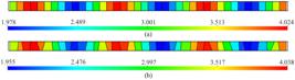
The results presented in Figure 9 show a remarkable similarity across the computational domain. This behavior was to be expected from the qualitative comparison, since the use of the orthogonal quadrilateral mesh reduces the MPFA-D method to the FD method. It is also known that the FD method is implemented in the MODFLOW 6 simulator.

Figure 9
(a) Hydraulic head field obtained using the FD/MPFA-D method and (b) using MODFLOW 6 with the M1 grid.

Figure 10 shows the distribution of hydraulic heads determined using the FD and MPFA-D methods. The dimensions of the elements containing the river and the recharge and pumping wells have not been distorted. In the orthogonal quadrilateral grid, the hydraulic heads in the wells were determined as follows: $h_1=\mathrm{944,7}\text{m}$, $h_2=\mathrm{155,6}\text{m}$ and $h_3=\mathrm{15,61}\text{m}$. For the distorted grid, the following hydraulic heads were determined using the MPFA-D method: $h_1=\mathrm{944,9}\text{m}$, $h_2=\mathrm{155,6}\text{m}$ and $h_3=\mathrm{15,05}\text{m}$. For the FD method, the hydraulic heads in the wells were determined as follows: $h_1=\mathrm{917,8}\text{m}$, $h_2=\mathrm{154,58}\text{m}$ and $h_3=\mathrm{15,69}\text{m}$. It can be observed that the FD method results in a lower hydraulic head in the recharge well, which shows a greater sensitivity to grid distortion. In contrast, the MPFA-D method showed greater robustness to distortions and kept the hydraulic heads close to those obtained with the orthogonal grid (see Figure 10). These results show that the MPFA-D method is able to preserve robustness even for distorted meshes and proves to be a more reliable approach for applications with complex geometries.

Figure 10
(a) Hydraulic head field obtained using the CVFD method and (b) hydraulic head field obtained using the MPFA-D method, both with the M2 mesh.

In Figure 11, the profile of hydraulic head along $y=22$ is analyzed, highlighting the stability of the MPFA-D method in both meshes, while the FD method shows inconsistencies in the M2 mesh, resulting in a profile that is relatively far from the others.

Figure 11
Hydraulic head profile obtained in $y=22\text{m}$.

Heterogeneous and anisotropic aquifer with river boundary

In this case, adapted from Farmani et al. (2023), a heterogeneous and anisotropic region is considered whose left boundary is delimited by a river with an infiltration rate of 0.24 m/day. The study domain is a rectangle with dimensions of 105 m in the y direction and 420 m in the x direction. This domain was divided into three sections, each with different hydraulic conductivity characteristics, as shown in Figure 12.

Figure 12
Physical domain and boundary conditions.

$$K_1=\left(\begin{array}{cc}1& 0\\ 0& 1.25\end{array}\right),K_2=\left(\begin{array}{cc}3.2& 0\\ 0& 2.75\end{array}\right)\text{and}{K}_3=\left(\begin{array}{cc}2.6& 0\\ 0& 3.5\end{array}\right)$$ (31)

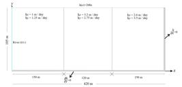
The presence of different physical properties in the domain is essential to adequately capture flow patterns, as each section affects the velocity and direction of water movement differently depending on variations in soil properties. The right and lower boundaries are impermeable, i.e. there is no water flow. At the upper boundary, a Dirichlet boundary condition is assumed where the hydraulic head varies linearly along x according to the $h=200x\text{m}$ equation, reflecting an increasing hydraulic gradient in the region.

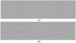
The computational mesh M1 shown in Figure 13(a) is an orthogonal quadrilateral, while Figure 13(b) shows a distorted version of this mesh. Both have 35 elements in the y direction and 140 in the x direction, totaling 4,900 control volumes.

Figure 13
(a) Orthogonal quadrilateral mesh and (b) distorted quadrilateral mesh.

Analysis of these results shows that the two methods for the M1 mesh have a high degree of agreement with the results of the MODFLOW6 simulator, as they have similar maximum and minimum values of hydraulic head, see Figure 14. This similarity shows the consistency of the numerical approaches in representing the hydraulic head in orthogonal quadrilateral mesh and emphasizes the reliability of the proposed methods. The results for the M2 mesh are also similar in this configuration. As shown in Figure 15, both the FD and MPFA-D methods show relatively stable performance.

Figure 14
(a) Hydraulic head field obtained from MPFA-D/FD method and (b) MODFLOW 6.

Figure 15
Hydraulic head field obtained with MPFA-D and FD methods, M2 mesh.

The graphical analysis shown in Figure 16 confirms that the methods used represent the behavior of hydraulic head in discontinuous porous media with greater robustness. It is also found that the profile obtained with the finite element method (FE) does not adequately represent the discontinuities of the material.

Figure 16
Hydraulic head profile in y= 0.01.

CONCLUSIONS

The results obtained in this study show the importance of choosing an appropriate numerical method for modeling groundwater flow, especially in geologically complex aquifers and when using distorted grids. The comparative analysis between the MPFA-D, FD methods and MODFLOW 6 showed that the three have similar performance on orthogonal grids, indicating a good ability to represent hydraulic head. However, when applied to distorted meshes, it can be observed that the behavior of the FD method differs significantly, with MPFA-D method showing greater accuracy and robustness of results. The superior performance of MPFA-D method is mainly due to its formulation, which allows a better representation of the heterogeneities and anisotropies of the porous medium. This feature is essential for practical applications in hydrogeological modeling, where the reliability of the results is crucial for decision making in water management.

ACKNOWLEDGEMENTS

The authors thank the Brazilian research agencies, especially CNPq, for supporting this work under grant 404517/2024-2.

DATA AVAILABILITY STATEMENT

Research data are available only upon request.

REFERENCES

• Aavatsmark, I. (2002). An introduction to multi-point flux approximations for quadrilateral grids. Computational Geosciences, 6(3–4), 405-432. https://doi.org/10.1023/A:1021291114475
  » https://doi.org/10.1023/A:1021291114475
• Aavatsmark, I., Barkve, T., Bøe, Ø., & Mannseth, T. (1996). Discretization on non-orthogonal, quadrilateral grids for inhomogeneous, anisotropic media. Journal of Computational Physics, 127(1), 2-14. https://doi.org/10.1006/jcph.1996.0154
  » https://doi.org/10.1006/jcph.1996.0154
• Aharmouch, A., Amaziane, B., El Ossmani, M., & Talali, K. (2020). A fully implicit finite volume scheme for a seawater intrusion problem in coastal aquifers. Water (Basel), 12(6), 1639. https://doi.org/10.3390/w12061639
  » https://doi.org/10.3390/w12061639
• Alecsa, C. D., Boros, I., Frank, F., Knabner, P., Nechita, M., Prechtel, A., Rupp, A., & Suciu, N. (2020). Numerical benchmark study for flow in highly heterogeneous aquifers. Advances in Water Resources, 138, 103558. https://doi.org/10.1016/j.advwatres.2020.103558
  » https://doi.org/10.1016/j.advwatres.2020.103558
• Bakker, M., & Post, V. (2022). Analytical groundwater modeling: theory and applications using Python (1st ed.). Boca Raton: CRC Press. https://doi.org/10.1201/9781315206134
  » https://doi.org/10.1201/9781315206134
• Bertolazzi, E., & Manzini, G. (2004). Least square-based finite volumes for solving the advection–diffusion of contaminants in porous media. Applied Numerical Mathematics, 51(4), 493-512. https://doi.org/10.1016/j.apnum.2004.10.003
  » https://doi.org/10.1016/j.apnum.2004.10.003
• Blazek, J. (2015). Computational fluid dynamics: principles and applications (3rd ed., 578 p.). Oxford: Butterworth-Heinemann.
• Cavalcante, T. M., Contreras, F., Lyra, P. R. M., & Carvalho, D. N. (2020). A multi-point flux approximation with diamond stencil finite volume scheme for the two-dimensional simulation of fluid flows in naturally fractured reservoirs using a hybrid-grid method. International Journal for Numerical Methods in Fluids, 92(10), 1322-1351. https://doi.org/10.1002/fld.4829
  » https://doi.org/10.1002/fld.4829
• Chen, Q.-Y., Wan, J., Yang, Y., & Mifflin, R. T. (2008). Enriched multi-point flux approximation for general grids. Journal of Computational Physics, 227(3), 1701-1721. https://doi.org/10.1016/j.jcp.2007.09.021
  » https://doi.org/10.1016/j.jcp.2007.09.021
• Chou, S.-H., & Ye, X. (2007). Superconvergence of finite volume methods for the second order elliptic problem. Computer Methods in Applied Mechanics and Engineering, 196(37-40), 3706-3712. https://doi.org/10.1016/j.cma.2006.10.025
  » https://doi.org/10.1016/j.cma.2006.10.025
• Contreras, F. R. L., Lyra, P. R. M., Souza, M. R. A., & Carvalho, D. K. E. (2016). A cell-centered multi-point flux approximation method with a diamond stencil coupled with a higher order finite volume method for the simulation of oil–water displacements in heterogeneous and anisotropic petroleum reservoirs. Computers & Fluids, 127, 1-16. https://doi.org/10.1016/j.compfluid.2015.11.013
  » https://doi.org/10.1016/j.compfluid.2015.11.013
• Contreras, F. R. L., Lyra, P. R. M., & Carvalho, D. K. E. (2019). A new multi-point flux approximation method with a quasi-local stencil (MPFA-QL) for the simulation of diffusion problems in anisotropic and heterogeneous media. Applied Mathematical Modelling, 70, 659-676. https://doi.org/10.1016/j.apm.2019.01.033
  » https://doi.org/10.1016/j.apm.2019.01.033
• Contreras, F. R. L., Carvalho, D. K. E., Galindez-Ramirez, G., & Lyra, P. R. M. (2021). A non-linear finite volume method coupled with a modified higher order MUSCL-type method for the numerical simulation of two-phase flows in non-homogeneous and non-isotropic oil reservoirs. Computers & Mathematics with Applications, 92, 120-133. https://doi.org/10.1016/j.camwa.2021.03.023
  » https://doi.org/10.1016/j.camwa.2021.03.023
• Contreras, F. R. L., Vaz, U. A. O., Pacheco, G. L. S. S., Antunes, A. R. E., Lyra, P. R. M., & Carvalho, D. K. E. (2023). A high-resolution multidimensional finite volume scheme coupled to a nonlinear two-point flux approximation method for the numerical simulation of groundwater contaminant transport using unstructured 2D meshes. Advances in Water Resources, 181, 104559. https://doi.org/10.1016/j.advwatres.2023.104559
  » https://doi.org/10.1016/j.advwatres.2023.104559
• Edwards, M. G., & Zheng, H. (2008). A quasi-positive family of continuous Darcy-flux finite-volume schemes with full pressure support. Journal of Computational Physics, 227(22), 9333-9364. https://doi.org/10.1016/j.jcp.2008.05.028
  » https://doi.org/10.1016/j.jcp.2008.05.028
• Farmani, S., Ghaeini-Hessaroeyeh, M., & Hamzehei-Javaran, S. (2023). Numerical model of seepage flows by reformulating finite element method based on new spherical Hankel shape functions. Applied Water Science, 13(8), 8. https://doi.org/10.1007/s13201-022-01813-1
  » https://doi.org/10.1007/s13201-022-01813-1
• Fetter, C. W. (2018). Applied hydrogeology (4th ed.) Long Grove: Waveland Press.
• Freeze, R. A., & Cherry, J. A. (1979). Groundwater Englewood Cliffs: Prentice-Hall.
• Friis, H. A., & Edwards, M. G. (2011). A family of MPFA finite-volume schemes with full pressure support for the general tensor pressure equation on cell-centred triangular grids. Journal of Computational Physics, 230(1), 205-231. https://doi.org/10.1016/j.jcp.2010.09.012
  » https://doi.org/10.1016/j.jcp.2010.09.012
• Gao, Z., & Wu, J. (2010). A linearity-preserving cell-centered scheme for the heterogeneous and anisotropic diffusion equations on general meshes. International Journal for Numerical Methods in Fluids, 67(12), 2157-2183. https://doi.org/10.1002/fld.2496
  » https://doi.org/10.1002/fld.2496
• Gao, Z., & Wu, J. (2013). A small stencil and extremum-preserving scheme for anisotropic diffusion problems on arbitrary 2D and 3D meshes. Journal of Computational Physics, 250, 308-331. https://doi.org/10.1016/j.jcp.2013.05.013
  » https://doi.org/10.1016/j.jcp.2013.05.013
• Gao, Y., Yi, S., & Zheng, C. (2021). Efficient simulation of groundwater solute transport using the multi-point flux approximation method with arbitrary polygon grids. Journal of Hydrology, 601, 126637. https://doi.org/10.1016/j.jhydrol.2021.126637
  » https://doi.org/10.1016/j.jhydrol.2021.126637
• Gao, Y., Du, E., Yi, S., Han, Y., & Zheng, C. (2022). An improved numerical model for groundwater flow simulation with MPFA method on arbitrary polygon grids. Journal of Hydrology, 606, 127399. https://doi.org/10.1016/j.jhydrol.2021.127399
  » https://doi.org/10.1016/j.jhydrol.2021.127399
• Igboekwe, M. U., & Achi, N. J. (2011). Finite difference method of modelling groundwater flow. Journal of Water Resource and Protection, 3(3), 192-198. https://doi.org/10.4236/jwarp.2011.33025
  » https://doi.org/10.4236/jwarp.2011.33025
• Instituto Trata Brasil. (2023). Retrieved in 2023, November 10, from https://www.tratabrasil.org.br
  » https://www.tratabrasil.org.br
• Klausen, R. A., Radu, F. A., & Eigestad, G. T. (2008). Convergence of MPFA on triangulations and for Richards’ equation. International Journal for Numerical Methods in Fluids, 58(12), 1327-1351. https://doi.org/10.1002/fld.1787
  » https://doi.org/10.1002/fld.1787
• Langevin, C. D., Hughes, J. D., Banta, E. R., Niswonger, R. G., Panday, S., & Provost, A. M. (2021). Documentation for the MODFLOW 6 groundwater flow model: techniques and methods 6-A55 (197 p.). Reston, VA: U.S. Geological Survey. https://doi.org/10.3133/tm6A55
  » https://doi.org/10.3133/tm6A55
• Li, L., Zhou, H., & Gómez-Hernández, J. J. (2010). Steady-state saturated groundwater flow modeling with full tensor conductivities using finite differences. Computers & Geosciences, 36(10), 1211-1223. https://doi.org/10.1016/j.cageo.2010.04.002
  » https://doi.org/10.1016/j.cageo.2010.04.002
• Maliska, C. R. (2004). Transferência de calor e mecânica dos fluidos computacional: fundamentos e coordenação numérica Rio de Janeiro: LTC.
• Maus, V. W. (2011). Modelagem computacional aplicada ao transporte de contaminantes em águas subterrâneas(Dissertação de mestrado). Universidade Federal de Juiz de Fora, Juiz de Fora.
• Muyinda, N., Kakuba, G., & Mango, J. M. (2014). Finite volume method of modelling transient groundwater flow. Journal of Mathematics and Statistics, 10(1), 92-110. https://doi.org/10.3844/jmssp.2014.92.110
  » https://doi.org/10.3844/jmssp.2014.92.110
• Pal, M., Edwards, M. G., & Lamb, A. R. (2006). Convergence study of a family of flux-continuous, finite-volume schemes for the general tensor pressure equation. International Journal for Numerical Methods in Fluids, 51(9-10), 1177-1203. https://doi.org/10.1002/fld.1211
  » https://doi.org/10.1002/fld.1211
• Qian, Y., Zhu, Y., Zhang, X., Wu, J., Ye, M., Mao, W., Wu, J., Huang, J., & Yang, J. (2023). A local grid-refined numerical groundwater model based on the vertex-centred finite-volume method. Advances in Water Resources, 173, 104392. https://doi.org/10.1016/j.advwatres.2023.104392
  » https://doi.org/10.1016/j.advwatres.2023.104392
• Silva, P. C. G., Pacheco, G. L. S. S., Albuquerque, P. V. P., Souza, M. R. A., Contreras, F. R. L., Lyra, P. R. M., & Carvalho, D. K. E. (2024). A modified Flux Corrected Transport method coupled with the MPFA-H formulation for the numerical simulation of two-phase flows in petroleum reservoirs using 2D unstructured meshes. Computational Geosciences, 28(6), 1149-1173. https://doi.org/10.1007/s10596-024-10306-w
  » https://doi.org/10.1007/s10596-024-10306-w
• Suk, H., Chen, J. S., Park, E., & Kihm, Y. H. (2020). Practical application of the Galerkin finite element method with a mass conservation scheme under Dirichlet boundary conditions to solve groundwater problems. Sustainability, 12(14), 5627. https://doi.org/10.3390/su12145627
  » https://doi.org/10.3390/su12145627
• Younes, A., Fahs, M., & Belfort, B. (2013). Monotonicity of the cell-centred triangular MPFA method for saturated and unsaturated flow in heterogeneous porous media. Journal of Hydrology, 504, 132-141. https://doi.org/10.1016/j.jhydrol.2013.09.041
  » https://doi.org/10.1016/j.jhydrol.2013.09.041
• Zhang, X., Zhu, Y., Wang, J., Ju, L., Qian, Y., Ye, M., & Yang, J. (2022). GW-PINN: A deep learning algorithm for solving groundwater flow equations. Advances in Water Resources, 165, 104243. https://doi.org/10.1016/j.advwatres.2022.104243
  » https://doi.org/10.1016/j.advwatres.2022.104243

Edited by

• Editor-in-Chief:
  Adilson Pinheiro

• Associated Editor:
  Edson Cezar Wendland

Publication Dates

• Publication in this collection
  02 Mar 2026
• Date of issue
  2026

History

• Received
  14 May 2025
• Reviewed
  02 Sept 2025
• Accepted
  15 Dec 2025