Rayleigh Waves: Velocity, Attenuation with Depth and Elliptical Polarization

Abstract

In 1887, Lord Rayleigh published a theory of a surface wave that later became known as the Rayleigh wave. The main features of this wave are its attenuation with depth and the fact that its velocity is always less than the S-wave velocity. Classical textbooks on elastic waves propagation and seismology usually consider the so-called Poisson solid, in which the Poisson’s ratio is equal to 0.25. In this study, we present some mathematical details and geometrical aspects that are not discussed in the textbooks. We obtain the Rayleigh cubic equation and compute its three roots as a function of the Poisson’s ratio. Then, we compute the particle displacements in a given depth, U(z) and W(z), as well as the instantaneous displacements, u(x, z, t) and w(x, z, t), to demonstrate the elliptical polarization of the particle motion and to indicate the rotation direction of the geometrical locus. We find that for each value of Poisson’s ratio, at a critical depth, the rotation direction changes from retrograde to prograde. Finally, we find the critical depth by three different approaches.

Keywords
Rayleigh wave; Poisson’s ratio; cubic equation; ellipse rotation direction; ellipse eccentricity

Introduction

In an unlimited, homogeneous, and isotropic solid medium there are two kinds of elastic body waves, known as P-waves (longitudinal, fast-traveling pressure waves) and S-waves (transverse, slow-traveling shear waves). Lord Rayleigh (John William Strut, 1842–1919) was a British physicist who made significant contributions to physics in the 19th and early 20th century, particularly in acoustics. He also won the Nobel Prize in Physics in 1904 for discovering Argon gas. His most important contribution to geophysics was the prediction of the existence of a surface wave if the solid is not unlimited. This wave, later called Rayleigh wave, has a rapidly decreasing amplitude with depth and a velocity less than that of body waves.

Surface waves are of great importance in both earthquake and exploration seismology. The common presence of Rayleigh wave in the seismic field data is usually considered a problem, when the Rayleigh wave, also known as ground roll, is treated as noise and must be removed or at least have its effect attenuated during the seismic processing stage.

Rayleigh presented his research results in 1885 and published them two years later in a British mathematical journal [¹]. His paper, which is also reproduced in Pellisier et al. [²], does not present modern mathematical notation. Thus, in this paper, we follow Kolsky’s [³] notation and approach.

Lord Rayleigh obtained a cubic equation, now known as the Rayleigh equation, whose roots can be related to the Poisson’s ratio ν. Poisson’s ratio is a dimensionless elastic parameter defined as the ratio of lateral contraction (normal strain ϵ_xx) to longitudinal extension (normal strain ϵ_zz) of a vertical bar under terminal tractive load, i.e., ν = −ϵ_xx/ϵ_zz. He considered four cases of Poisson’s ratio, including the Poisson’s solid (ν = 0.25), and also the case of ν = −1, which is not considered in many areas of knowledge, including geophysics. He ends his study stating that it is not improbable that the surface waves here investigated play an important part in earthquakes.

Classical textbooks on elastic wave propagation and seismology usually consider the case of the Poisson’s solid, or eventually the case of steel, with ν = 0.29. The root with physical meaning of the cubic equation for the Poisson’s solid is 0.9194, which means that the surface wave velocity c is 0.9194 times the value of S-wave velocity c_S.

In a two-page and one figure paper, Knopoff [⁴] studied this problem and made velocity ratio curves as a function of ν. Some textbooks, for instance, Ewing et al. [⁵], Graff [⁶] and Miklowitz [⁷], reproduced Knopoff’s results. Kolsky [³] produced the particle displacement curves for the case of steel. Also, Viktorov [⁸] presented the displacement curves for ν = 0.25 and ν = 0.34, stating that the values of the Poisson’s ratio for most metals lie between these values. Graff [⁶], Miklowitz [⁷] and Achenbach [⁹] all reproduced his curves in their textbooks.

We present some mathematical details and geometrical aspects that are not discussed in the textbooks. Considering a 2–D half-space limited by an interface with a homogeneous and isotropic solid medium below the interface, we obtain the Rayleigh cubic equation and compute its three roots as a function of the Poisson’s ratio, varying ν from 0 to 0.5. We conclude that only one root has physical meaning for each value of Poisson’s ratio. Royer [¹⁰] also presented the three roots with their real and imaginary parts. We also compute the particle displacements in a given depth, U(z) and W(z), as well as the instantaneous displacements u(x, z, t) and w(x, z, t), to plot the elliptical polarization curves of the particle motion and to indicate the rotation direction of the geometrical locus on the curves.

For each value of ν, the rotation direction changes from retrograde to prograde at a critical depth z_C. We find z_C by three approaches, computing the depth z: (i) at which the ellipse contracts into a pure vertical motion when its eccentricity equals to 1; (ii) at which the value of the derivative dRe[w(x, z, t)]/dRe[u(x, z, t)] changes from positive to negative; and (iii) at which the horizontal displacement U(z) is zero.

In this study, we consider only the Rayleigh wave which attenuates with depth, thus having a physical meaning. The complex roots lead to the so-called leaking modes, which are discussed in some books and papers, such as Hudson [¹¹], Schröder & Scott Jr. [¹²] and Chapman [¹³].

Theory

Surface wave equations

The equations of elastodynamics are given by [³]:

(1) $$\rho \frac{{\partial }^{2}u}{\partial t^2}=(\lambda +\mu )\frac{\partial \mathrm{\Delta }}{\partial x}+\mu {\nabla }^{2}u,$$

(2) $$\rho \frac{{\partial }^{2}v}{\partial t^2}=(\lambda +\mu )\frac{\partial \mathrm{\Delta }}{\partial y}+\mu {\nabla }^{2}v,$$

and

(3) $$\rho \frac{{\partial }^{2}w}{\partial t^2}=(\lambda +\mu )\frac{\partial \mathrm{\Delta }}{\partial z}+\mu {\nabla }^{2}w.$$

where u, v and w are the displacements in relation to the x, y, and z axes, respectively. λ and μ are the Lamé constants (SI unit N/m² or Pascal), which completely define the elastic behavior of an isotropic medium. Δ is the dilatation and μ is also known as rigidity.

Consider an elastic medium with a plane limit expressed by z equal to a constant, e.g., z = 0, so that the surface wave is confined to the vicinity of this plane limit, as illustrated in Figure 1. We consider a wave propagating along the x-axis, with displacements that are invariant in relation to the y-axis.

FIGURE 1
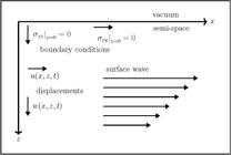
Diagram of a Rayleigh wave whose amplitude decreases with depth, with oriented axes x and z, displacements u and w and stress boundary conditions that vanish at the surface.

The Helmholtz decomposition or theorem will be useful in this study. The displacement vector u can be decomposed into two independent auxiliary potentials, the scalar potential ϕ and the vector potential Ψ:

$$\mathbf{\text{u}}=\nabla \varphi +\nabla \times \mathbf{\Psi }.$$

One additional condition, ∇ ⋅ Ψ = 0, provides the unique determination of the three components of vector u. With the invariance in relation to the y-axis, the displacement vector is $\mathit{\text{u}}=u\widehat{\mathit{\text{i}}}+w\widehat{\mathit{\text{k}}}$. Also, the vector potential Ψ has only non-zero component in relation to y-axis, that is, $\mathbf{\Psi }=-\psi \widehat{\mathit{\text{j}}}$, hence being associated to rotation in the x − z plane. The negative sign is adopted for convenience. Thus, we obtain the following relations between the auxiliary potentials, ϕ and ψ, and the displacements u and w:

(4) $$u=\frac{\partial \varphi }{\partial x}+\frac{\partial \psi }{\partial z},\text{and}\mathit{}w=\frac{\partial \varphi }{\partial z}-\frac{\partial \psi }{\partial x}.$$

By expressing displacement as a 2-D vector, $\mathbf{\text{u}}=u\widehat{\mathit{\text{i}}}+w\widehat{\mathit{\text{k}}}$, we can obtain the dilatation, which represents the relative volume variation in a solid, and defined by Δ = ∇ ⋅ u. Thus,

(5) $$\mathrm{\Delta }=\left(\frac{\partial }{\partial x}\widehat{\mathit{\text{i}}}+\frac{\partial }{\partial z}\widehat{\mathit{\text{k}}}\right)\cdot \left(u\widehat{\mathit{\text{i}}}+w\widehat{\mathit{\text{k}}}\right)=\frac{\partial u}{\partial x}+\frac{\partial w}{\partial z}={ϵ}_{xx}+{ϵ}_{zz},$$

in which the normal strains are ϵ_xx and ϵ_zz, and we considered ∂⁡v/∂⁡y = 0. Normal strain, for example, ϵ_xx, is a dimensionless measure of the infinitesimal contraction or expansion of a particle in a plane given by x = constant (first subscript) and in the direction of the x-axis (second subscript). The dilatation can be expressed in terms of auxiliary potentials by substituting equation (4) into equation (5):

(6) $$\mathrm{\Delta }=\frac{{\partial }^2\varphi }{\partial x^2}+\frac{{\partial }^2\varphi }{\partial z^2}={\nabla }^2\varphi .$$

The rotation in the plane xz (along the y-axis) is defined as follows [³]:

(7) $$2{\overline{\omega }}_y=\frac{\partial u}{\partial z}-\frac{\partial w}{\partial x}.$$

Substituting equation (4) into equation (7), we have the following:

(8) $$2{\overline{\omega }}_y=\frac{{\partial }^2\psi }{\partial x^2}+\frac{{\partial }^2\psi }{\partial z^2}={\nabla }^2\psi .$$

Thus, the potential ϕ is associated with the wave dilatation, and the potential ψ is associated with its rotation. The introduction of these two potentials allows us to separate the effects related to dilatation from those related to rotation.

Substituting equations (4) and (6) into equations (1) and (3), respectively:

(9) $$\rho {\displaystyle \frac{{\partial }^2}{\partial t^2}}\left({\displaystyle \frac{\partial \varphi }{\partial x}}+{\displaystyle \frac{\partial \psi }{\partial z}}\right)=(\lambda +\mu ){\displaystyle \frac{\partial }{\partial x}}({\nabla }^2\varphi )+\mu {\nabla }^2\left({\displaystyle \frac{\partial \varphi }{\partial x}}+{\displaystyle \frac{\partial \psi }{\partial z}}\right),$$

and

(10) $$\rho {\displaystyle \frac{{\partial }^2}{\partial t^2}}\left({\displaystyle \frac{\partial \varphi }{\partial z}}-{\displaystyle \frac{\partial \psi }{\partial x}}\right)=(\lambda +\mu ){\displaystyle \frac{\partial }{\partial z}}({\nabla }^2\varphi )+\mu {\nabla }^2\left({\displaystyle \frac{\partial \varphi }{\partial z}}-{\displaystyle \frac{\partial \psi }{\partial x}}\right).$$

The equations (9) and (10) can be rewritten as follows:

(11) $$\rho {\displaystyle \frac{\partial }{\partial x}}\left({\displaystyle \frac{{\partial }^2\varphi }{\partial t^2}}\right)+\rho {\displaystyle \frac{\partial }{\partial z}}\left({\displaystyle \frac{{\partial }^2\psi }{\partial t^2}}\right)=(\lambda +2\mu ){\displaystyle \frac{\partial }{\partial x}}({\nabla }^2\varphi )+\mu {\displaystyle \frac{\partial }{\partial z}}({\nabla }^2\psi ),$$

and

(12) $$\rho {\displaystyle \frac{\partial }{\partial z}}\left({\displaystyle \frac{{\partial }^2\varphi }{\partial t^2}}\right)-\rho {\displaystyle \frac{\partial }{\partial x}}\left({\displaystyle \frac{{\partial }^2\psi }{\partial t^2}}\right)=(\lambda +2\mu ){\displaystyle \frac{\partial }{\partial z}}({\nabla }^2\varphi )-\mu {\displaystyle \frac{\partial }{\partial x}}({\nabla }^2\psi ).$$

We separate the functions ϕ and ψ on each side of equations (11) and (12) :

$$\rho \frac{\partial }{\partial x}\left(\frac{{\partial }^2\varphi }{\partial t^2}\right)-(\lambda +2\mu )\frac{\partial }{\partial x}({\nabla }^2\varphi )=-\rho \frac{\partial }{\partial z}\left(\frac{{\partial }^2\psi }{\partial t^2}\right)+\mu \frac{\partial }{\partial z}({\nabla }^2\psi ),$$

and

$$\rho \frac{\partial }{\partial z}\left(\frac{{\partial }^2\varphi }{\partial t^2}\right)-(\lambda +2\mu )\frac{\partial }{\partial z}({\nabla }^2\varphi )=\rho \frac{\partial }{\partial x}\left(\frac{{\partial }^2\psi }{\partial t^2}\right)-\mu \frac{\partial }{\partial x}({\nabla }^2\psi ).$$

The above equations can be rearranjed as

$$\frac{\partial }{\partial x}\left[\rho \frac{{\partial }^2\varphi }{\partial t^2}-(\lambda +2\mu ){\nabla }^2\varphi \right]=\frac{\partial }{\partial z}\left(\mu {\nabla }^2\psi -\rho \frac{{\partial }^2\psi }{\partial t^2}\right),$$

and

$$\frac{\partial }{\partial z}\left[\rho \frac{{\partial }^2\varphi }{\partial t^2}-(\lambda +2\mu ){\nabla }^2\varphi \right]=\frac{\partial }{\partial x}\left(\rho \frac{{\partial }^2\psi }{\partial t^2}-\mu {\nabla }^2\psi \right).$$

Since the functions are ϕ and ψ independent, each side of the equations should equal a constant, e.g., E and H:

$$\{\begin{array}{c}\frac{\partial }{\partial x}\left[\rho \frac{{\partial }^2\varphi }{\partial t^2}-(\lambda +2\mu ){\nabla }^2\varphi \right]=E,\hfill \\ \\ \frac{\partial }{\partial z}\left(\mu {\nabla }^2\psi -\rho \frac{{\partial }^2\psi }{\partial t^2}\right)=E,\hfill \end{array}$$

and

$$\{\begin{array}{c}\frac{\partial }{\partial z}\left[\rho \frac{{\partial }^2\varphi }{\partial t^2}-(\lambda +2\mu ){\nabla }^2\varphi \right]=H,\hfill \\ \\ \frac{\partial }{\partial x}\left(\rho \frac{{\partial }^2\psi }{\partial t^2}-\mu {\nabla }^2\psi \right)=H.\hfill \end{array}$$

After the integration by x and z in each system of differential equations, we have the following:

$$\{\begin{array}{c}\rho \frac{{\partial }^2\varphi }{\partial t^2}-(\lambda +2\mu ){\nabla }^2\varphi =E(z),\hfill \\ \\ \mu {\nabla }^2\psi -\rho \frac{{\partial }^2\psi }{\partial t^2}=E(x),\hfill \end{array}$$

and

$$\{\begin{array}{c}\rho \frac{{\partial }^2\varphi }{\partial t^2}-(\lambda +2\mu ){\nabla }^2\varphi =H(x),\hfill \\ \\ \rho \frac{{\partial }^2\psi }{\partial t^2}-\mu {\nabla }^2\psi =H(z).\hfill \end{array}$$

The constants vanish since the coordinates x and z are independent. Thus, we obtain two wave equations:

(13) $${\nabla }^2\varphi =\frac{1}{c_P^2}\frac{{\partial }^2\varphi }{\partial t^2},c_P=\sqrt{\frac{\lambda +2\mu }{\rho }},$$

and

(14) $${\nabla }^2\psi =\frac{1}{c_S^2}\frac{{\partial }^2\psi }{\partial t^2},c_S=\sqrt{\frac{\mu }{\rho }},$$

in which c_P is the compressional wave velocity and c_S is the shear wave velocity.

Solutions of the wave equations and boundary conditions

If we consider a sinusoidal wave which propagates along the x-axis, in which c is the surface wave velocity, we obtain the following the solution to equation (13):

(15) $$\varphi (x,z,t)=F(z)e^{i(\omega t-kx)},$$

and the solution to equation (14):

(16) $$\psi (x,z,t)=G(z)e^{i(\omega t-kx)}.$$

In the Ansatzes solutions given by equations (15) and (16), F(z) and G(z) are non-specified functions that express the wave amplitude variations with the depth. The angular frequency ω present in both solutions is dependent on the wavenumber k (ω = ck), and k is determined by the wavelength λ (k = 2π/λ).

We determine the second derivatives of ϕ in relation to x, y and t, and introduce them into equation (13), which leads to an ordinary differential equation for F(z):

(17) $$F^{″}(z)-(k^2-k_P^2)F(z)=0,$$

in which k_P = ω/c_P. Equation (17) associated characteristic equation is

(18) $$q^2=(k^2-k_P^2),$$

and its roots are

(19) $$q_1=-q=-\sqrt{k^2-k_P^2},\text{and}\mathit{}{q}_2=q=\sqrt{k^2-k_P^2}.$$

As a result, the differential equation solution is

$$F(z)=A{e}^{-qz}+A^{\prime }{e}^{qz}.$$

It should be noted that A′e^qz represents a wave whose amplitude increases with depth, with no physical consistency. Therefore, A′ must be zero, and the solution becomes as follows:

(20) $$F(z)=A{e}^{-qz}.$$

Following the same steps for the potential ψ, we obtain the ordinary differential equation

(21) $$G^{″}(z)-(k^2-k_S^2)G(z)=0,$$

if k_S = ω/c_S. Equation (21) associated characteristic equation is

(22) $$s^2=(k^2-k_S^2),$$

and its roots are

(23) $$s_1=-s=-\sqrt{k^2-k_S^2},\text{and}\mathit{}{s}_2=s=\sqrt{k^2-k_S^2}.$$

Again, the positive root represents a wave whose amplitude increases with depth, without being physically consistency. Hence, the solution is

(24) $$G(z)=B{e}^{-sz}.$$

By substituting equation (20) into equation (15), the potential ϕ solution is:

(25) $$\varphi (x,z,t)=A{e}^{-qz}{e}^{i(\omega t-kx)}.$$

Similarly, by substituting equation (24) into equation (16), the potential ψ solution is:

(26) $$\psi (x,z,t)=B{e}^{-sz}{e}^{i(\omega t-kx)}.$$

The half-space interface is represented by the plane xy at z = 0. At this plane, due to the absence of matter above the surface, the boundary conditions of the stress are:

(27) $${{\sigma }_{zz}|}_{z=0}=0,{{\sigma }_{zy}|}_{z=0}=0,{{\sigma }_{zx}|}_{z=0}=0.$$

The condition σ_zy = 0 is not necessary because we assume invariance with respect to the y-axis.

For a homogeneous and isotropic solid, Hooke’s law is given by:

$$\left(\begin{array}{c}{\sigma }_{xx}\\ {\sigma }_{yy}\\ {\sigma }_{zz}\\ {\sigma }_{yz}\\ {\sigma }_{zx}\\ {\sigma }_{xy}\end{array}\right)=\left(\begin{array}{cccccc}\lambda +2\mu & \lambda & \lambda & 0& 0& 0\\ \lambda & \lambda +2\mu & \lambda & 0& 0& 0\\ \lambda & \lambda & \lambda +2\mu & 0& 0& 0\\ 0& 0& 0& \mu & 0& 0\\ 0& 0& 0& 0& \mu & 0\\ 0& 0& 0& 0& 0& \mu \end{array}\right)\times \left(\begin{array}{c}{ϵ}_{xx}\\ {ϵ}_{yy}\\ {ϵ}_{zz}\\ {ϵ}_{yz}\\ {ϵ}_{zx}\\ {ϵ}_{xy}\end{array}\right).$$

For the 2–D case, the normal stress σ_zz is given by the third row of the above system, i.e.:

(28) $${\sigma }_{zz}=\lambda \mathrm{\Delta }+2\mu {ϵ}_{zz}=\lambda \frac{\partial u}{\partial x}+(\lambda +2\mu )\frac{\partial w}{\partial z}.$$

The first right-hand side partial derivative of equation (28) is given by:

(29) $$\frac{\partial u}{\partial x}=\frac{\partial }{\partial x}\left(\frac{\partial \varphi }{\partial x}+\frac{\partial \psi }{\partial z}\right)=\frac{{\partial }^2\varphi }{\partial x^2}+\frac{{\partial }^2\psi }{\partial x\partial z}.$$

By using equations (25) and (26) in equation (29), we obtain the following:

(30) $$\frac{\partial u}{\partial x}=-k^{2}A{e}^{-qz}{e}^{i(\omega t-kx)}+iksB{e}^{-sz}{e}^{i(\omega t-kx)}.$$

At the interface z = 0, equation (30) becomes as follows:

(31) $${\frac{\partial u}{\partial x}|}_{z=0}=-k^{2}A{e}^{i(\omega t-kx)}+iksB{e}^{i(\omega t-kx)}.$$

The second right-hand side partial derivative of equation (28) is expressed by:

(32) $$\frac{\partial w}{\partial z}=\frac{\partial }{\partial z}\left(\frac{\partial \varphi }{\partial z}-\frac{\partial \psi }{\partial x}\right)=\frac{{\partial }^2\varphi }{\partial z^2}-\frac{{\partial }^2\psi }{\partial z\partial x}.$$

Similarly, by using equations (25) and (26) in equation (32), we have the following:

(33) $$\frac{\partial w}{\partial z}=q^{2}A{e}^{-qz}{e}^{i(\omega t-kx)}-iksB{e}^{-sz}{e}^{i(\omega t-kx)}.$$

At the interface z = 0, equation (33) becomes as follows:

(34) $${\frac{\partial w}{\partial z}|}_{z=0}=q^{2}A{e}^{i(\omega t-kx)}-iksB{e}^{i(\omega t-kx)}.$$

Finally, the condition σ_zz = 0 results in:

(35) $$A[(\lambda +2\mu )q^2-\lambda k^2]-2B\mu isk=0.$$

Hooke’s law and the potentials ϕ and ψ also express the shear stress σ_zx:

$${\sigma }_{zx}=\mu {ϵ}_{zx}=\mu \left(\frac{\partial u}{\partial z}+\frac{\partial w}{\partial x}\right)$$ $$\mathrm{}=\mu \left(\frac{{\partial }^2\psi }{\partial z^2}-\frac{{\partial }^2\psi }{\partial x^2}+2\frac{{\partial }^2\varphi }{\partial z\partial x}\right),$$

or

(36) $${\sigma }_{zx}=\mathrm{}\mu [s^{2}B{e}^{-sz}{e}^{i(\omega t-kx)}+k^{2}B{e}^{-sz}{e}^{i(\omega t-kx)}+2ikqA{e}^{-qz}{e}^{i(\omega t-kx)}].$$

At the interface z = 0, equation (36) becomes:

$${\sigma }_{zx}{|}_{z=0}=\mu [s^{2}B{e}^{i(\omega t-kx)}+k^{2}B{e}^{i(\omega t-kx)}\mathrm{}+2ikqA{e}^{i(\omega t-kx)}]=0,$$

or

(37) $$2iqkA+(s^2+k^2)B=0.$$

Rayleigh equation

By applying the first boundary condition given by equation (35), we obtain the following:

(38) $$\frac{A}{B}=\frac{2\mu isk}{[(\lambda +2\mu )q^2-\lambda k^2]}.$$

While utilizing the second boundary condition from equation (37), we come to the following:

(39) $$\frac{A}{B}=\frac{(s^2+k^2)}{-2iqk}.$$

By combining equations (38) and (39), we obtain the following:

$$4\mu qs{k}^2=[(\lambda +2\mu )q^2-\lambda k^2](s^2+k^2),$$

or

(40) $$16{\mu }^2(k^2-k_P^2)(k^2-k_S^2)k^4={[-(\lambda +2\mu )k_P^2+2\mu k^2]}^2{(2k^2-k_S^2)}^2,$$

with $q^2=k^2-k_P^2$ and $s^2=k^2-k_S^2$.

Then, we isolate μ² at the right-hand side of equation (40) and simplify it as follows:

(41) $$16(k^2-k_P^2)(k^2-k_S^2)k^4={[-(\lambda +2\mu ){\mu }^{-1}{k}_P^2+2k^2]}^2{(2k^2-k_S^2)}^2.$$

Next, we divide all terms by k², then cut k⁸ from both sides of equation (41):

(42) $$16\left(1-{\displaystyle \frac{k_P^2}{k^2}}\right)\left(1-{\displaystyle \frac{k_S^2}{k^2}}\right)={\left[-(\lambda +2\mu ){\mu }^{-1}{\displaystyle \frac{k_P^2}{k^2}}+2\right]}^2{\left(2-{\displaystyle \frac{k_S^2}{k^2}}\right)}^2.$$

On the other hand, if k_P = ω/c_P and k_S = ω/c_S, then we can have the following relation:

(43) $$\frac{k_P^2}{k_S^2}=\frac{{\omega }^2/c_P^2}{{\omega }^2/c_S^2}=\frac{c_S^2}{c_P^2}=\frac{\mu /\rho }{(\lambda +2\mu )/\rho }=\frac{\mu }{\lambda +2\mu }.$$

Let us make α₁ = k_P/k_S and substitute the result of equation (43) into equation (42):

(44) $$16\left(1-{\alpha }_1^2{\displaystyle \frac{k_S^2}{k^2}}\right)\left(1-{\displaystyle \frac{k_S^2}{k^2}}\right)={\left(2-{\displaystyle \frac{k_S^2}{k^2}}\right)}^2{\left(2-{\displaystyle \frac{k_S^2}{k^2}}\right)}^2={\left(2-{\displaystyle \frac{k_S^2}{k^2}}\right)}^4.$$

Now, we define γ = k_S/k so that equation (44) becomes

$$16(1-{\alpha }_1^2{\gamma }^2)(1-{\gamma }^2)={(2-{\gamma }^2)}^4,$$

or

(45) $${({\gamma }^2)}^3-8{({\gamma }^2)}^2+(24-16{\alpha }_1^2){\gamma }^2+16{\alpha }_1^2-16=0.$$

Equation (45) is known as the Rayleigh equation. Finally, we can express the variable γ as follows:

$$\gamma =\frac{k_S}{k}=\frac{\omega /c_S}{\omega /c}=\frac{c}{c_S}.$$

Numerical Simulations

Poisson’s ratio, its range and the Poisson’s solid

From the definition of α₁ and the equation (43), we can have the following:

(46) $${\alpha }_1^2=\frac{k_P^2}{k_S^2}=\frac{\mu }{\lambda +2\mu }.$$

Using Hooke’s law in the definition ν = −ϵ_xx/ϵ_zz, we have the following [³]:

(47) $$\nu =\frac{\lambda }{2(\lambda +\mu )}.$$

We want to express α₁ in terms of ν. We isolate μ and λ + 2μ in equation (47) as follows:

(48) $$\mu =\frac{1-2\nu }{2\nu }\lambda \mathit{}\text{and}\mathit{}\lambda +2\mu =\frac{1-\nu }{\nu }\lambda .$$

By substituting the expressions from equation (48) into equation (46), we obtain the following:

(49) $${\alpha }_1^2=\frac{1-2\nu }{2-2\nu }.$$

To establish the Poisson’s ratio range, we isolate the Lamé’s constant λ in equation (47):

(50) $$2\mu \nu =\lambda (1-2\nu ).$$

Both sides of equation (50) are positive. This implies that ν ≤ 1/2, which means that ν_max = 0.5. On the other hand, if λ = 0 at the right-hand side of equation (50), then ν = 0 at the left-side hand, which means that ν_min = 0.

Many seismological problems are simplified by assuming that λ = μ. Such a material, called a Poisson solid, is often a good approximation for the earth. In this case, Poisson’s ratio is ν = 1/4 [¹⁴]. Using equation (49), we obtain ${\alpha }_1^2=1/3$. For this value of ${\alpha }_1^2$, equation (45) becomes

$$3{({\gamma }^2)}^3-24{({\gamma }^2)}^2+56{\gamma }^2-32=0,$$

or

$$[{\gamma }^2-4][3{({\gamma }^2)}^2-12({\gamma }^2)+8]=0,$$

and its roots are

$${\gamma }_1^2=4,{\gamma }_2^2=2+\frac{2}{\sqrt{3}}=3.1547,\text{and}\mathrm{}{\gamma }_3^2=2-\frac{2}{\sqrt{3}}=0.8453.$$

The roots ${\gamma }_1^2$ and ${\gamma }_2^2$ lead to complex values in the F(z) and G(z) expressions. Thus, the only possible root is ${\gamma }_3^2$ = 0.8453, or γ₃ = 0.9194, which means that the surface wave velocity c is 0.9194 times the value of the shear wave velocity c_S.

Computation of roots and velocities

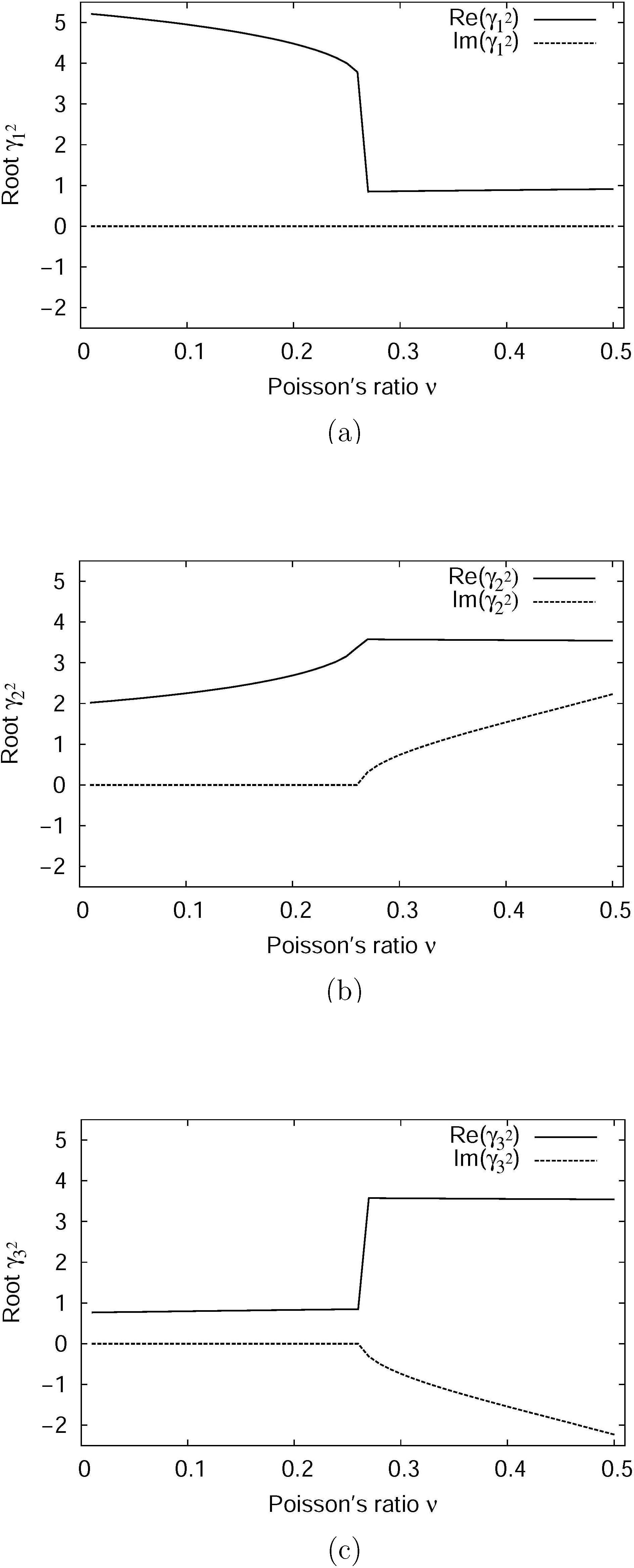
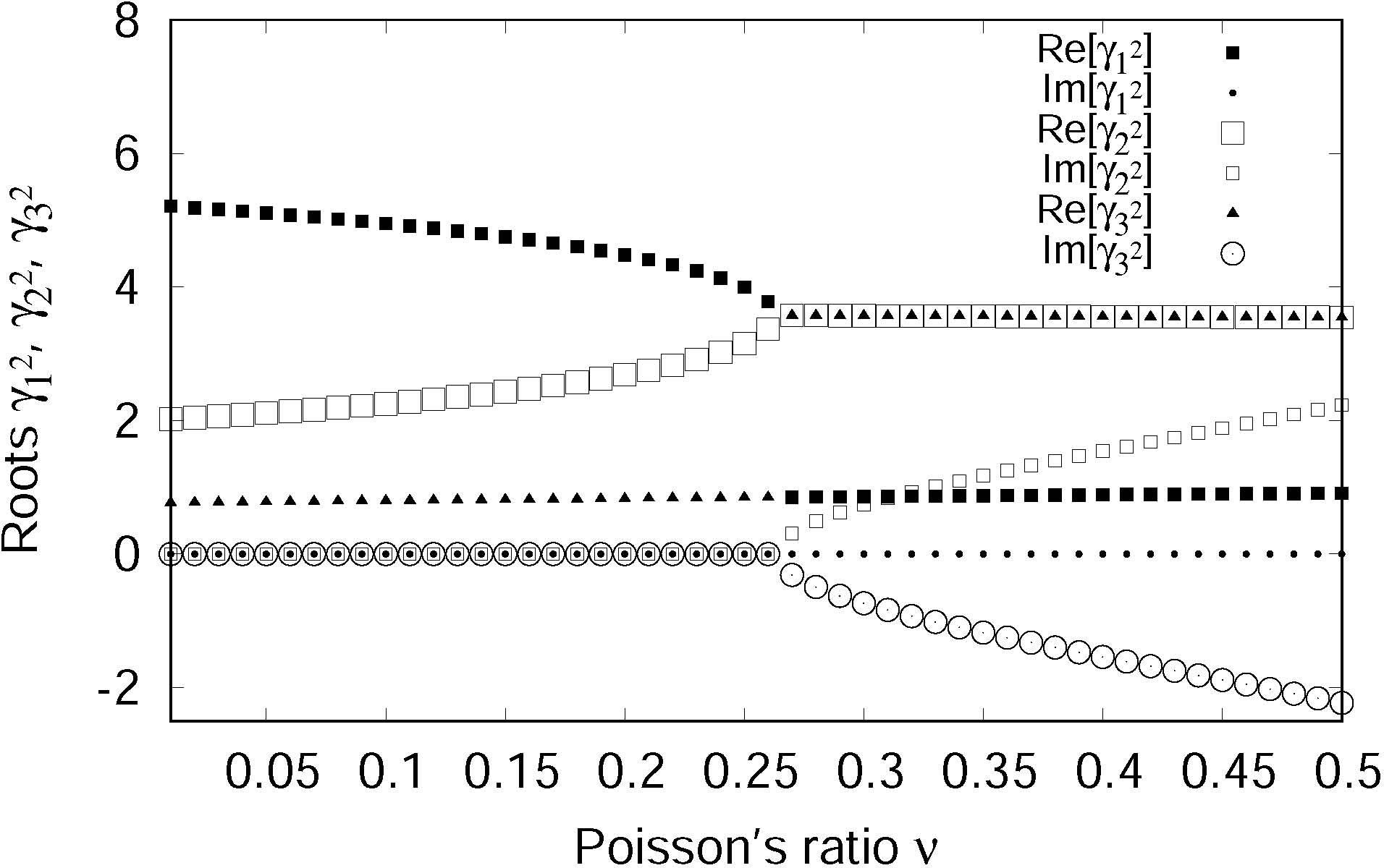
By setting Δν = 0.01, we have 50 Poisson’s ratio values, from ν = 0.01 up to ν = 0.50. We calculate ${\alpha }_1^2$ for each value of ν and compute the three roots of the Rayleigh equation using the classical method described in Annex 1. Figure 2 illustrates the relationship between α₁ and γ, while Figure 3 displays the values of the three roots. Because the roots are generally complex, two curves are presented for each root. The six curves in Figure 3 can be superimposed, as displayed in Figure 4. This result was first presented by Royer [¹⁰].

FIGURE 2
Factor α₁ = c_S/c_P as a function of the root γ = c/c_S.

FIGURE 3
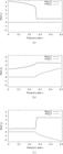
Real and imaginary parts of the Rayleigh equation roots as a function of the Poisson’s ratio ν: (a) first root, ${\gamma }_1^2$, (b) second root,${\gamma }_1^2$, (c) third root,${\gamma }_3^2$.

FIGURE 4
Real and imaginary parts of the Rayleigh equation roots, ${\gamma }_1^2$, ${\gamma }_2^2$ and ${\gamma }_3^2$, as function of the Poisson’s ratio ν.

In this study, we only consider the roots with physical meaning. According to equation (18), the condition k > k_P is necessary to obtain a real positive q, which represents a surface wave that attenuates with depth. On the other hand, the condition k > k_P leads to c < c_P. According to equation (22), we also need k > k_S to have a real positive s, which again represents a surface wave which attenuates with depth. Similarly, the condition k > k_S leads to c < c_S, which is equivalent to γ = c/c_S < 1.

As seen in Figure 3(a), the first root is always real, that is, $\text{Im}({\gamma }_1^2)=0$. The second root, ${\gamma }_2^2$, in Figure 3(b), is real if ν < 0.264 (see Appendix A). Also, the third root, ${\gamma }_3^2$, in Figure 3(c), is real if ν < 0.264. To ensure that the condition γ < 1 is satisfied, we select root ${\gamma }_3^2$ values in the range ν = [0.01,0.26], and then ${\gamma }_1^2$ values in the range ν = [0.26,0.50].

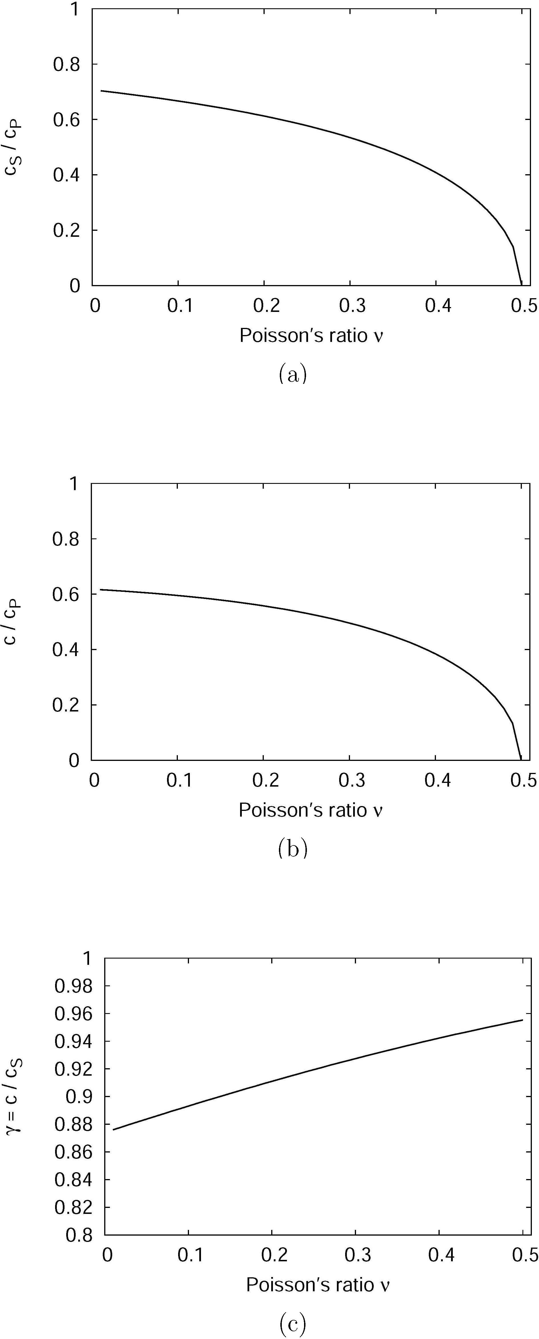
In a two-page and one figure short paper, Knopoff [⁴] studied this problem and derived the velocity ratio curves as a function of ν. Some classical textbooks of elastic wave propagation reproduce Knopoff’s results, for instance, Ewing et al. [⁵, p. 340], Graff [⁶, p. 326] and Miklowitz [⁷, p. 148]. Figure 5(a) illustrates the ratio c_S/c_P as a Poisson’s ratio function, while Figures 5(b) and 5(c) display the ratios c/c_P and c/c_S as Poisson’s ratio functions, respectively. Figure 5(c) presents a limited range for the Rayleigh wave velocity c, ranging from 88% to 94% of the S-wave velocity c_S.

FIGURE 5
Velocity ratios as a function of Poisson’s ratio ν ranging from 0.01 to 0.50: (a) c_S/c_P, (b) c/c_P, (c) c/c_S.

Attenuation with depth

In a homogeneous, isotropic half-space the surface wave propagates without dispersion, because the mathematical relation between the Rayleigh wave velocity c and the S-wave velocity c_S (γ = c/c_S) is univocal and does not involve angular frequency ω. The γ ratio depends only on Poisson’s ratio ν, which is constant for a given half-space. However, even in an ideal medium, there is attenuation with depth z. This attenuation is represented by the indexes q and s, which are present in the expressions of displacements u and w. Thus, from equation (4) we have the following:

(51) $$u(x,z,t)=(-iAk{e}^{-qz}-Bs{e}^{-sz})e^{i(\omega t-kx)},$$

and

(52) $$w(x,z,t)=(-Aq{e}^{-qz}+iBk{e}^{-sz})e^{i(\omega t-kx)}.$$

By substituting equation (37) into equations (51) and (52), we have, respectively:

(53) $$u(x,z,t)=Aik\left[-e^{-qz}+2qs{(s^2+k^2)}^{-1}{e}^{-sz}\right]e^{i(\omega t-kx)},$$

and

(54) $$w(x,z,t)=Aq\left[-e^{-qz}+2k^2{(s^2+k^2)}^{-1}{e}^{-sz}\right]e^{i(\omega t-kx)}.$$

Using Euler relation, e^i(ωt−kx) = cos⁡(ωt − kx) + i sin⁡(ωt−kx), and taking the real part from equation (53) we have the following equation:

(55) $$Re[u(x,z,t)]=U(z)\sin (\omega t-kx),$$

in which

(56) $$U(z)=Ak[e^{-qz}-2qs{(s^2+k^2)}^{-1}{e}^{-sz}].$$

And, from equation (54) we have that:

(57) $$Re[w(x,z,t)=W(z)\cos (\omega t-kx),$$

in which

(58) $$W(z)=Aq[-e^{-qz}+2k^2{(s^2+k^2)}^{-1}{e}^{-sz}].$$

From equation (18) we have that

$$\frac{q^2}{k^2}=1-\frac{k_P^2}{k^2}=1-{\alpha }_1^2{\gamma }^2,$$

in which α₁ = k_P/k_S and γ = k_S/k. Thus,

(59) $$q=k\sqrt{1-{\alpha }_1^2{\gamma }^2}=k\beta ,$$

in which $\beta =\sqrt{1-{\alpha }_1^2{\gamma }^2}.$

Similarly, from equation (22) we have the following:

$$\frac{s^2}{k^2}=1-\frac{k_S^2}{k^2}=1-{\gamma }^2,$$

in which γ = k_S/k. Thus,

(60) $$s=k\sqrt{1-{\gamma }^2}=k\delta ,$$

in which $\delta =\sqrt{1-{\gamma }^2}.$

The Rayleigh wave will not attenuate with depth if s is complex. Consequently, the parameter s has to be real, which, again, implies the condition γ < 1.

By using equations (59) and (60) in equation (56), we obtain:

(61) $$U(z)=\mathrm{}{\displaystyle \frac{2\pi A}{\lambda }}[\exp (-2\pi \beta {\displaystyle \frac{z}{\lambda }})\mathrm{}-2\beta \delta {({\delta }^2+1)}^{-1}\exp (-2\pi \delta {\displaystyle \frac{z}{\lambda }})],$$

in which k = 2π/λ.

Similarly, using equations (59) and (60) into equation (58):

(62) $$W(z)=\mathrm{}{\displaystyle \frac{2\pi \beta A}{\lambda }}[-\exp (-2\pi \beta {\displaystyle \frac{z}{\lambda }})+2{({\delta }^2+1)}^{-1}\exp (-2\pi \delta {\displaystyle \frac{z}{\lambda }})].$$

Equations (61) and (62) can be normalized by the vertical displacement at the surface. If z = 0:

$$W(0)=\frac{2\pi \beta A}{\lambda }\left[-1+2{({\delta }^2+1)}^{-1}\right].$$

Thus,

(63) $${\displaystyle \frac{U(z)}{W(0)}}={\displaystyle \frac{\beta \left[\exp \left(-2\pi \beta {\displaystyle \frac{z}{\lambda }}\right)-2\beta \delta {({\delta }^2+1)}^{-1}\exp \left(-2\pi \delta {\displaystyle \frac{z}{\lambda }}\right)\right]}{\left[-1+2{({\delta }^2+1)}^{-1}\right]}},$$

and

(64) $${\displaystyle \frac{W(z)}{W(0)}}={\displaystyle \frac{\left[-\exp \left(-2\pi \beta {\displaystyle \frac{z}{\lambda }}\right)+2{({\delta }^2+1)}^{-1}\exp \left(-2\pi \delta {\displaystyle \frac{z}{\lambda }}\right)\right]}{\left[-1+2{({\delta }^2+1)}^{-1}\right]}}.$$

Alternatively, displacement U(z) can also be normalized by its correspondent displacement at the surface. If z = 0:

$$U(0)=\frac{2\pi A}{\lambda }\left[1-2\beta \delta {({\delta }^2+1)}^{-1}\right],$$

and

(65) $${\displaystyle \frac{U(z)}{U(0)}}={\displaystyle \frac{\left[\exp \left(-2\pi \beta {\displaystyle \frac{z}{\lambda }}\right)-2\beta \delta {({\delta }^2+1)}^{-1}\exp \left(-2\pi \delta \frac{z}{\lambda }\right)\right]}{\left[1-2\beta \delta {({\delta }^2+1)}^{-1}\right]}}.$$

By using equations (63) and (64), Kolsky [³, p. 22] produced the displacement curves for the case of steel (ν = 0.29). With the same equations, Viktorov [⁸, p. 5] displayed the curves for ν = 0.25 (Poisson’s solid) and also ν = 0.34, stating that between these values are the Poisson’s ratio values for most metals. His results are reproduced in Graff’s [⁶, p. 327], Miklowitz’s [⁷, p. 150] and Achenbach’s [⁹, p. 192] textbooks.

The range for ν used by Viktorov [⁸] is rather limited, although suitable for geophysical applications. Therefore, it would be interesting to check the behavior of the curves for other ν values. Besides the Poisson’s solid, we consider both a low and a high ν value. Figure 6 shows the Rayleigh wave displacement in the horizontal direction, U(z), as a function of relative depth z/λ, for Poisson’s ratio ν = 0.05, ν = 0.25 and ν = 0.45. This displacement was carried out without normalization in Figure 6(a) using equation (61), with normalization by W(0) in Figure 6(b) using equation (63), and with normalization by U(0) in Figure 6(c) using equation (65). And for the same three Poisson’s ratios, the vertical displacement, W(z) is shown in Figure 7: without normalization in Figure 7(a) using equation (62) and with normalization by W(0) in Figure 7(b) using equation (64). All curves presented in Figures 6 and 7 have an asymptotic behavior with depth, which is consistent with a surface wave, in which the energy is concentrated in the surface region.

FIGURE 6
Rayleigh wave particle motion in the horizontal direction, U(z), as a function of relative depth z/λ, for different values of Poisson’s ratio ν: (a) without normalization, (b) with normalization by W(0), (c) with normalization by U(0).

FIGURE 7
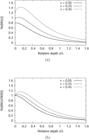
Rayleigh wave particle motion in the vertical direction, W(z), as a function of relative depth z/λ, for different values of Poisson’s ratio ν: (a) without normalization, (b) with normalization by W(0).

Elliptical polarization

Rayleigh waves show a unique behavior in the elastic wave propagation, which is the elliptical polarization of displacement components. From equation (55) we have that:

$$\sin (\omega t-kx)=\frac{Re[u(x,z,t)]}{U(z)},$$

and from equation (57) we can write the following:

$$\cos (\omega t-kx)=\frac{Re[w(x,z,t)]}{W(z)}.$$

By using sin²⁡(ωt − kx) + cos²⁡(ωt − kx) = 1, we obtain the following:

(66) $$\frac{Re{[u(x,z,t)]}^2}{{[U(z)]}^2}+\frac{Re{[w(x,z,t)]}^2}{{[W(z)]}^2}=1,$$

which is the equation of an ellipse, where U(z) and W(z) are its semi-axes.

Using the normalization defined by the equations (64) and (65) :

(67) $$\frac{Re{[u(x,z,t)]}^2}{{[U(z)/U(0)]}^2}+\frac{Re{[w(x,z,t)]}^2}{{[W(z)/W(0)]}^2}=1.$$

We calculate the amplitudes and rotation directions of the elliptical trajectories, for different values of ν and for different relative depths for a given ν. We considered x = 0 in equation (67) for the plotting of all ellipses in such a way that the phase becomes θ = ωt, or in a discrete form,

$${\theta }_k=2\pi \frac{t_k}{T}=2\pi \frac{k\mathrm{\Delta }t}{T}.$$

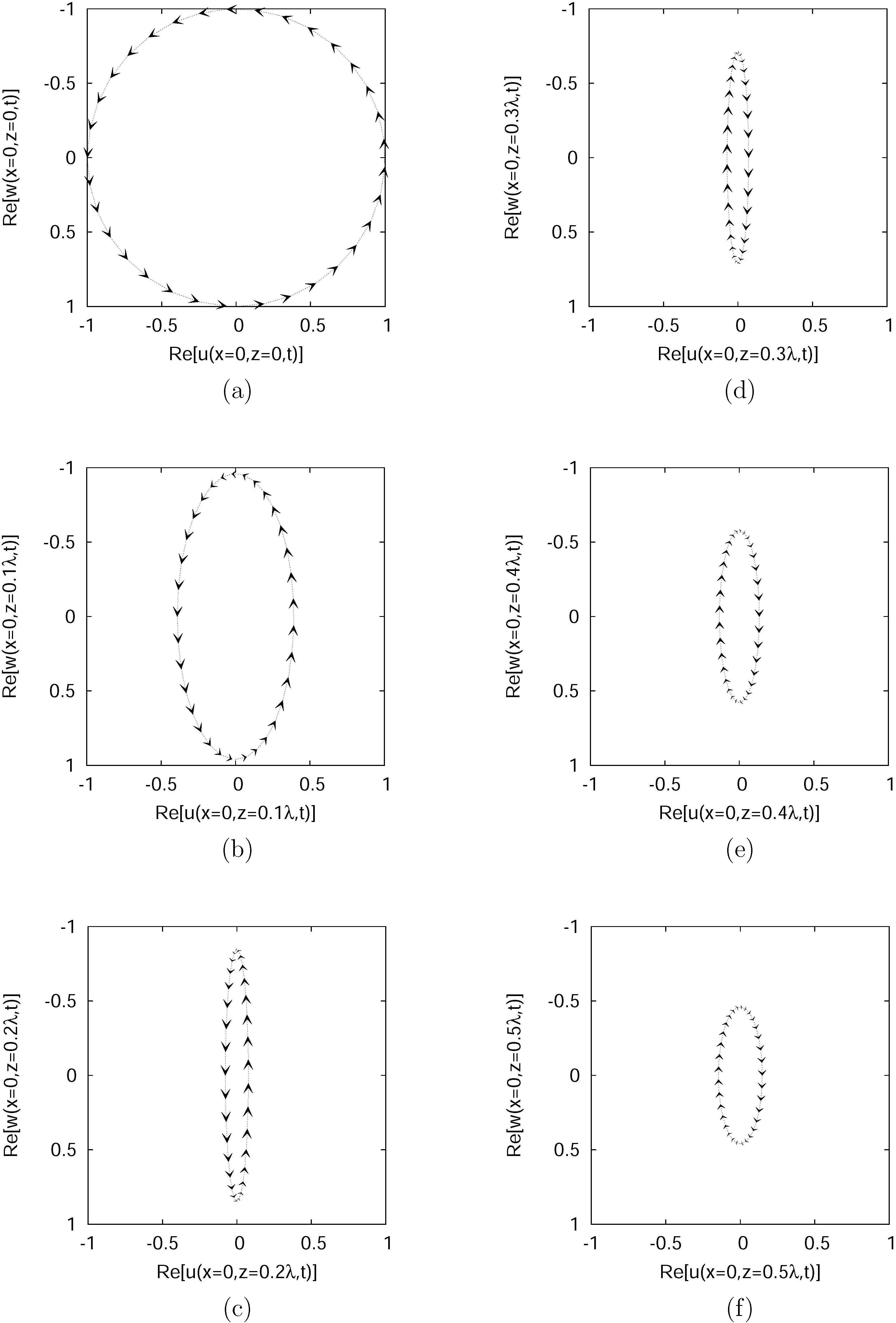
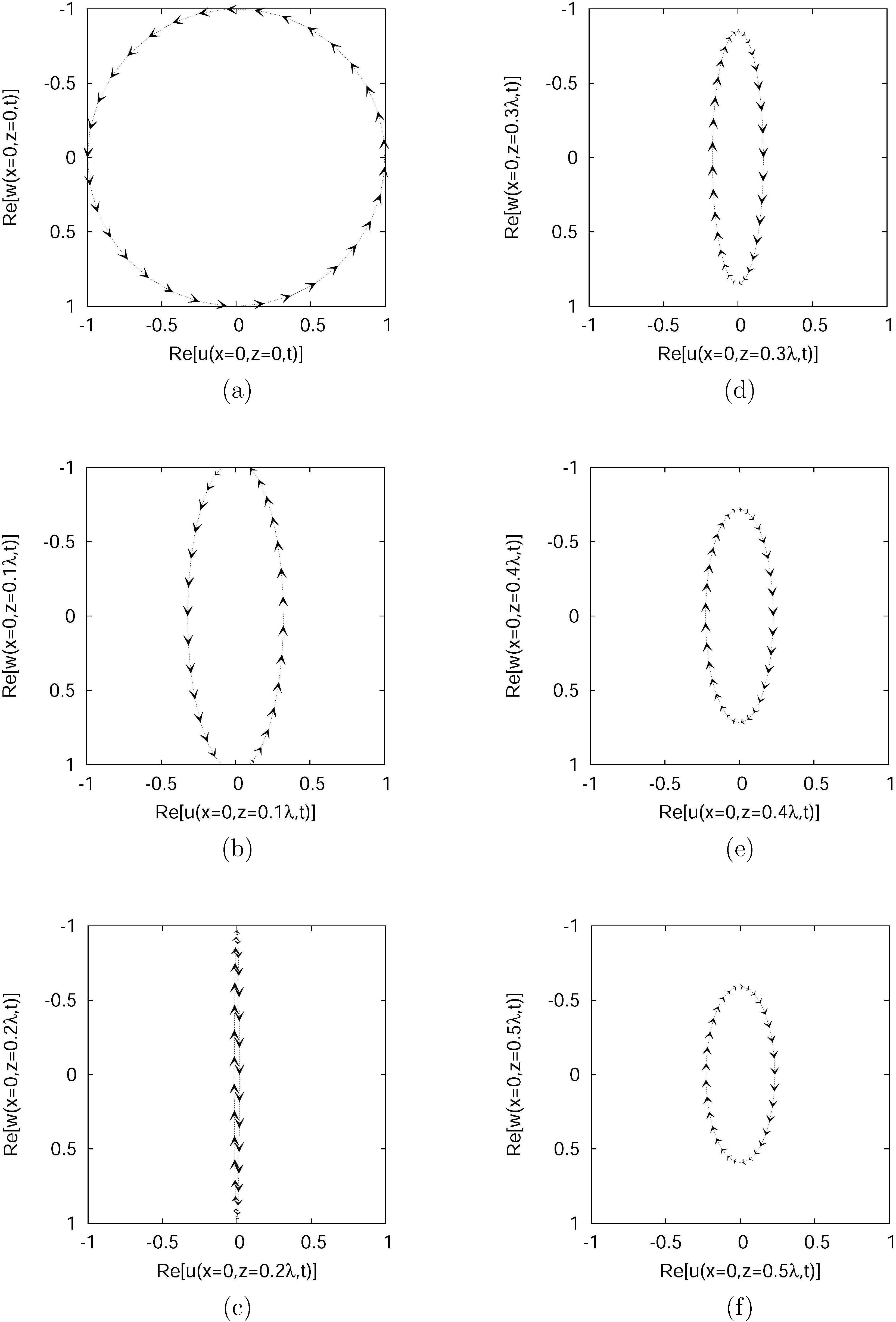
We adopted Δt = 0.01 s, which resulted in θ_k = 0.02πk, k = 1, 100. Figure 8 shows the Rayleigh wave elliptical polarization for Poisson’s ratio ν = 0.05, for six relative depths: from z = 0 in Figure 8(a) to z = 0.50λ in Figure 8(f). There is the retrograde motion for z = 0, z = 0.10λ and z = 0.20λ, and the prograde motion for z = 0.30λ, z = 0.40λ and z = 0.50λ. In other words, the behavior change happens in some depth between z = 0.20λ and z = 0.30λ. Because of the normalization, the amplitudes (ellipse semi-axes) at the surface, in both vertical and horizontal directions, are equal to 1.0 in Figure 8(a), which results in a circle.

FIGURE 8
Normalized amplitudes particle motion elliptical trajectory with Poisson’s ratio ν = 0.05 for different relative depths: (a) z = 0, (b) z = 0.1λ, (c) z = 0.2λ, (d) z = 0.3λ, (e) z = 0.4λ, (f) z = 0.5λ. Notice that the particle motion changes from retrograde to prograde between z = 0.2λ and z = 0.3λ.

For Poisson’s ratio ν = 0.25 (Poisson’s solid), and the same six depths, a similar array of ellipses appears in Figure 9. A slight increase in the amplitudes of U(z) and W(z) is noted when comparing the results at a given depth, for ν = 0.25 with those for ν = 0.05. This is due to the fact that γ increases with ν, which by its turn implies into an increase in the factor 2(δ² + 1)⁻¹ = 2(2 − γ²)⁻¹, present in both the expressions for U(z) and W(z).

FIGURE 9
Normalized amplitudes particle motion elliptical trajectory with Poisson’s ratio ν = 0.25 for different relative depths: (a) z = 0, (b) z = 0.1λ, (c) z = 0.2λ, (d) z = 0.3λ, (e) z = 0.4λ, (f) z = 0.5λ. Notice that the particle motion changes from retrograde to prograde between z = 0.1λ and z = 0.2λ.

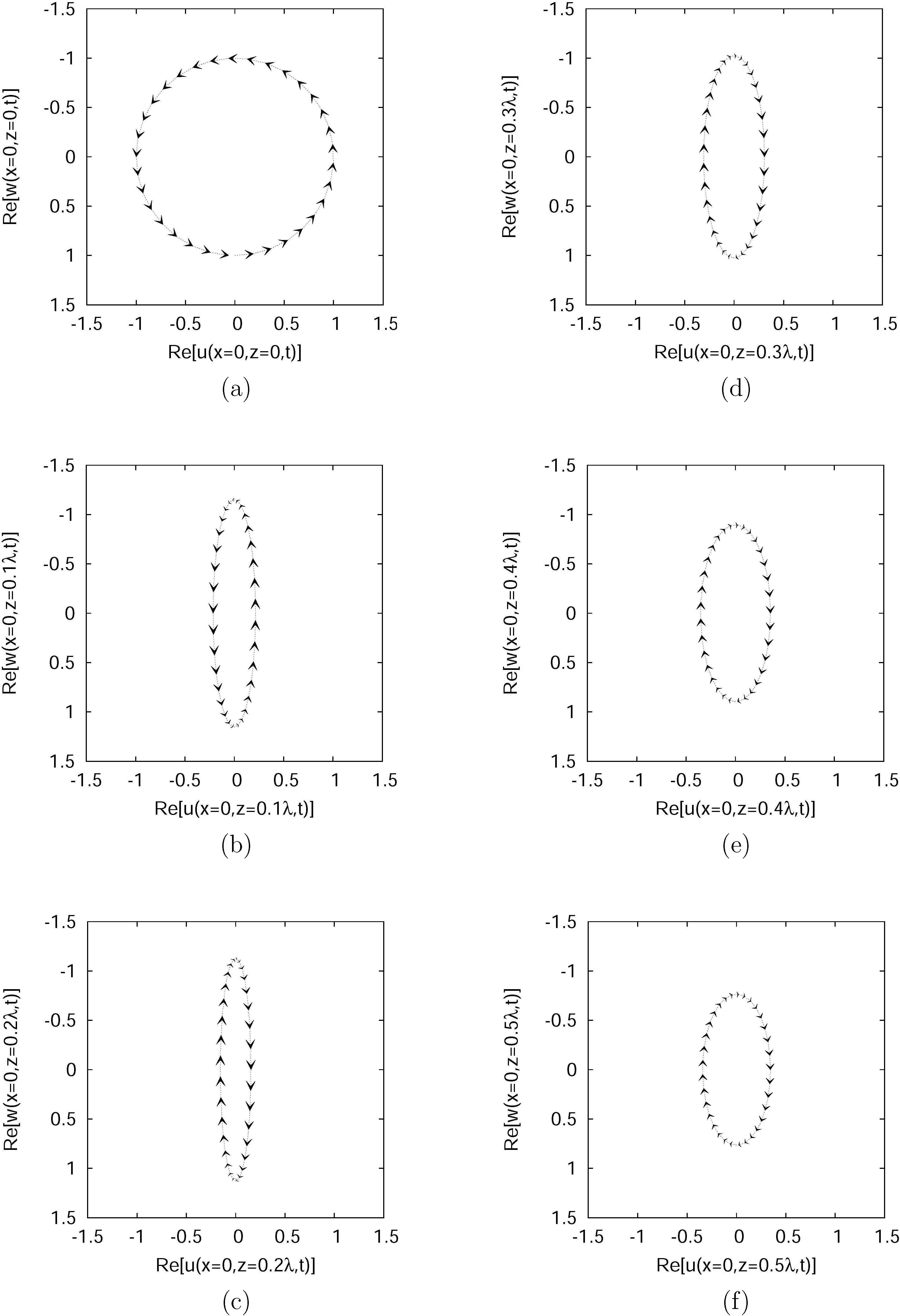
The results for a high Poisson’s ratio (ν = 0.45) are presented in Figure 10. For the same reason, there is a slight increase in the amplitudes of U(z) and W(z) when comparing the results at a given depth, for ν = 0.45 with those for ν = 0.25. In fact, it was necessary to modify the scale, due to the fact that most semi-axes were greater than 1.0.

FIGURE 10
Normalized amplitudes particle motion elliptical trajectory with Poisson’s ratio ν = 0.45 for different relative depths: (a) z = 0, (b) z = 0.1λ, (c) z = 0.2λ, (d) z = 0.3λ, (e) z = 0.4λ, (f) z = 0.5λ. Notice that the particle motion changes from retrograde to prograde between z = 0.1λ and z = 0.2λ.

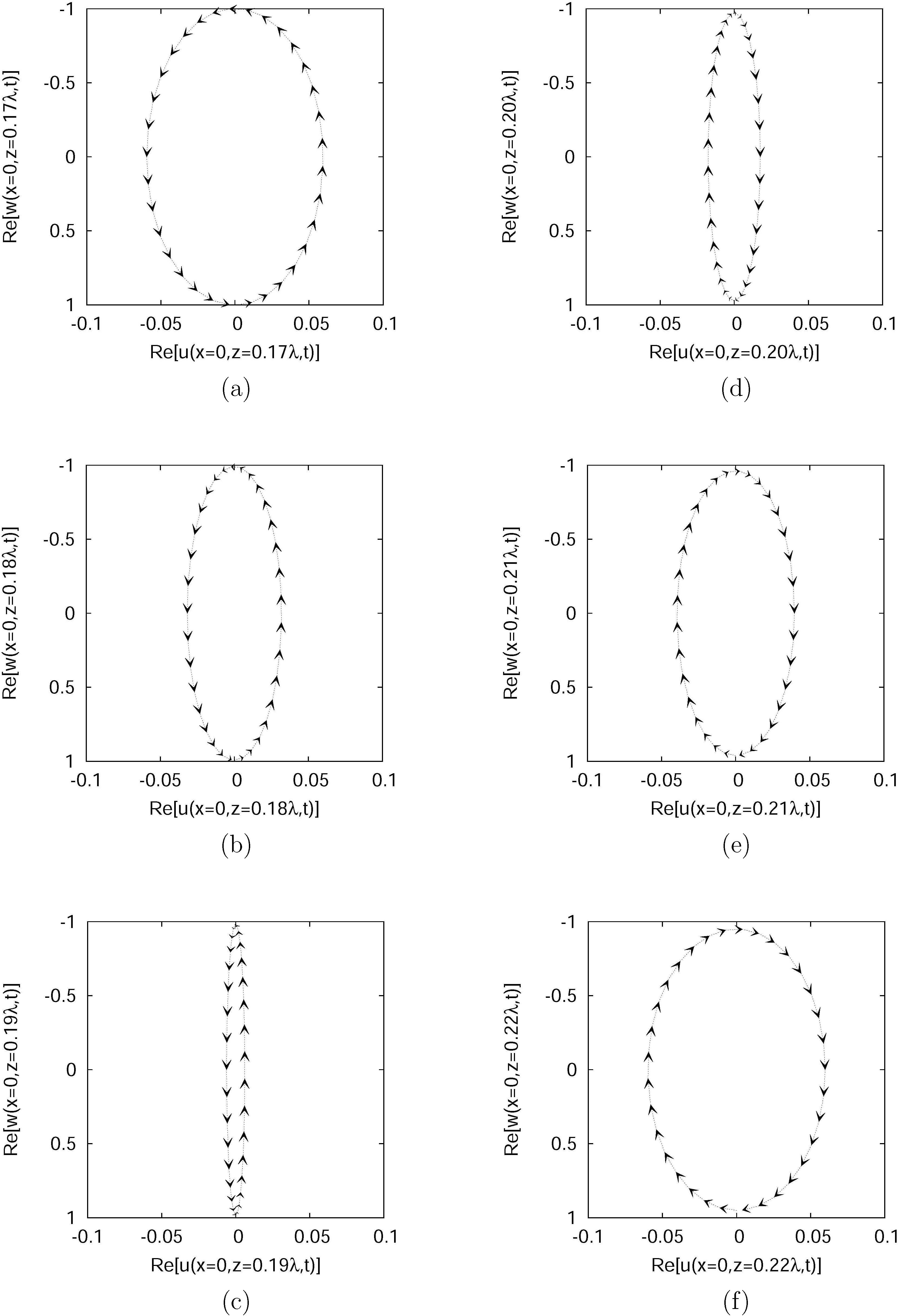
Finally, the rotation change in the ellipse can be analyzed in detail. For this, we will consider only the case ν = 0.25. The motion becomes prograde at some point between z = 0.10λ and z = 0.20λ, as indicated in Figure 9. Figure 11 shows the Rayleigh wave elliptical polarization with Poisson’s ratio ν = 0.25 for six relative depths, from z = 0.17λ in Figure 11(a) to z = 0.22λ in Figure 11(f). By comparing it with Figure 9, the horizontal scale is now exaggerated 5×. Also, the particle motion changes from retrograde to prograde between z = 0.19λ and z = 0.20λ, which is closer to z = 0.19λ.

FIGURE 11
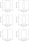
Normalized amplitudes particle motion elliptical trajectory with Poisson’s ratio ν = 0.25 for the relative depths: (a) z = 0.17λ, (b) z = 0.18λ, (c) z = 0.19λ, (d) z = 0.20λ, (e) z = 0.21λ, (f) z = 0.22λ. Notice that the when compared to Figure 9 the horizontal scale is exaggerated 5×. Notice also that the particle motion changes from retrograde to prograde between z = 0.19λ and z = 0.20λ.

The determination of the critical depth, when the ellipse movement changes the rotation direction from retrograde to prograde, is presented in Appendix B. Another interesting detail, which is the depth at which the ellipse has the longest vertical semi-axis, is discussed in Appendix C.

Conclusions

Rayleigh waves are very important in both earthquake and exploration seismology. In this study, we showed some mathematical details and geometrical aspects not discussed in the textbooks. We derived the Rayleigh cubic equation and computed its roots as a function of the Poisson’s ratio ν. We also computed the particle displacements, plotted the elliptical polarization of the particle motion and indicated the rotation direction at the geometrical locus. We observed that each value of ν, the rotation direction changes from retrograde to prograde towards a critical depth z_C. We obtained the value of z_C by three approaches. Finally, we determined the depth a which the ellipse has the maximum vertical semi-axis.

Acknowledgments

The author would like to thank CNPq for funding the project National Institute of Science and Technology of Petroleum Geophysics (INCT-GP).

Annex 1: Solution of the Cubic Equation

The method presented here is available in several Mathematics textbook, for example, Griffiths [¹⁵] and Birkhoff & Mac Lane [¹⁶]. Consider the cubic equation

(1.1) $$a{x}^3+b{x}^2+cx+d=0,$$

in which a, b, c and d are real constants. Dividing all the coefficients by a, we obtain the following result:

(1.2) $$x^3+\frac{b}{a}{x}^2+\frac{c}{a}x+\frac{d}{a}=0.$$

We now insert an auxiliary variable y:

(1.3) $$x=y-\frac{b}{3a},$$

into equation (1.2), obtaining:

$$y^3+\left(\frac{c}{a}-\frac{b^2}{3a^2}\right)y+\left(\frac{2b^3}{27a^3}-\frac{bc}{3a^2}+\frac{d}{a}\right)=0,$$

or

(1.4) $$y^3+Cy+D=0,$$

where

$$C=\frac{c}{a}-\frac{b^2}{3a^2},$$

and

$$D=\frac{2b^3}{27a^3}-\frac{bc}{3a^2}+\frac{d}{a}.$$

Equation (1.4) is known as reduced cubic equation. When a second auxiliary variable, z, expressed by:

(1.5) $$y=z-\frac{C}{3z},$$

with z ≠ 0, is used in equation (1.4), the result is expressed by:

$$z^3-\frac{C^3}{27z^3}+D=0,$$

or

(1.6) $$z^6+D{z}^3-\frac{C^3}{27}=0,$$

with C ≠ 0.

In equation (1.6), we use a third substitution, expressed by z³ = w, resulting in

(1.7) $$w^2+Dw-\frac{C^3}{27}=0.$$

Equation (1.7) is a quadratic equation with the following roots:

$$w_1=\frac{-D+\sqrt{D^2+4C^3/27}}{2},$$

and

$$w_2=\frac{-D-\sqrt{D^2+4C^3/27}}{2}.$$

Thus, the roots of equation (1.6) are

$$z_1^3=z_2^3=z_3^3=\frac{-D+\sqrt{D^2+4C^3/27}}{2},$$

and

$$z_4^3=z_5^3=z_6^3=\frac{-D-\sqrt{D^2+4C^3/27}}{2}.$$

If we multiply $z_1^3$ by $z_4^3$, we obtain

$$z_1^3{z}_4^3=-\frac{C^3}{27},$$

or

(1.8) $$z_1{z}_4=-\frac{C}{3}.$$

By substituting equation (1.8) into equation (1.5), we get:

$$y_1=z_1-\frac{C}{3z_1}=z_1+z_4,$$

or

$$y_1=\sqrt[3]{\frac{-D+\sqrt{D^2+4C^3/27}}{2}}+\sqrt[3]{\frac{-D-\sqrt{D^2+4C^3/27}}{2}}.$$

The root y₄ is

$$y_4=z_4-\frac{C}{3z_4}=z_4+z_1=y_1.$$

The same procedure can be applied to the other roots, that is, y₂ = y₅ and y₃ = y₆. Subsequently, we calculate the real root of the equation (1.1) using the equation (1.3):

$$x_1=y_1-\frac{b}{3a}.$$

With the root x₁, we can decompose the cubic equation as follows:

$$a{x}^3+b{x}^2+cx+d=(x-x_1)(a{x}^2+b_{1}x+c_1),$$

in which

$$b_1=a{x}_1+b,$$

and

$$c_1=a{x}_1^2+b{x}_1+c.$$

Finally, we can obtain the other two roots, x₂ and x₃ by using the well-known formula:

$$x_2=\frac{-b_1+\sqrt{b_1^2-4a{c}_1}}{2a},$$

and

$$x_3=\frac{-b_1-\sqrt{b_1^2-4a{c}_1}}{2a}.$$

Appendix A: The Limit Value ν = 0.263

In Annex 1 we saw that the reduced cubic equation is,

$$y^3+Cy+D=0.$$

Its discriminant Δ can be expressed [¹⁶, p. 120] as:

(A1) $$\mathrm{\Delta }=-4C^3-27D^2.$$

The following theorem is useful for this study. A quadratic or cubic equation with real coefficients has real roots if its discriminant is non-negative, and two imaginary roots if its discriminant is negative [¹⁶, p. 120].

Thus, for real roots, we have that Δ ≥ 0, or

(A2) $$-4C^3\ge 27D^2.$$

The coefficients of the equation (45) are:

$$a=1,b=-8,c=24-16{\alpha }_1^2,\text{and}\mathit{}d=16{\alpha }_1^2-16.$$

Thus, by using the expressions for C and D from Annex 1, we have

(A3) $$C=\frac{c}{a}-\frac{b^2}{3a^2}=\frac{8}{3}(1-6{\alpha }_1^2),$$

and

(A4) $$D=\frac{2b^3}{27a^3}-\frac{bc}{3a^2}+\frac{d}{a}=\frac{16}{27}\left(17-45{\alpha }_1^2\right).$$

By substituting equation (A3) and (A4) into equation (A2), we obtain

(A5) $${\left(12{\alpha }_1^2-2\right)}^3\ge {\left(17-45{\alpha }_1^2\right)}^2.$$

Let us consider the limit case, Δ = 0, so that equation (A5) becomes,

(A6) $${\left(12{\alpha }_1^2-2\right)}^3={\left(17-45{\alpha }_1^2\right)}^2,$$

or

(A7) $$192{({\alpha }_1^2)}^3-321{({\alpha }_1^2)}^2+186({\alpha }_1^2)-33=0.$$

Equation (A7) is a cubic equation in $({\alpha }_1^2)$, and its roots can be determined by the method described in Annex 1:

$${({\alpha }_1^2)}_1=0.3214,{({\alpha }_1^2)}_2=0.6752+i0.2806,\text{and}{({\alpha }_1^2)}_3=0.6752-i0.2806.$$

The second and third roots do not have physical meaning, otherwise they would lead to complex velocities.

The value ${\alpha }_1^2$ as a function of ν was expressed in equation (49). The reciprocal of this relation, that is, the value of ν as a function of ${\alpha }_1^2$ is then:

(A8) $$\nu =\frac{1-2{\alpha }_1^2}{2-2{\alpha }_1^2}.$$

By substituting ${({\alpha }_1^2)}_1=0.3214$ in equation (A8), we have

(A9) $$\nu ={\nu }_{limit}=0.26308.$$

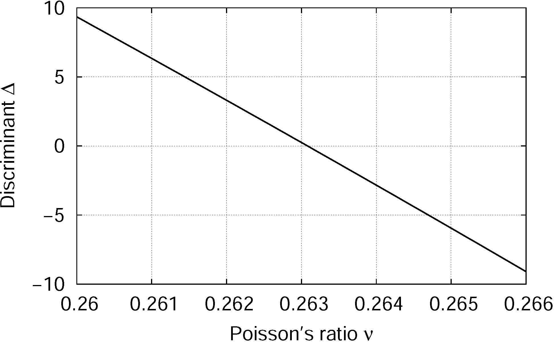
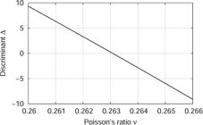
In conclusion, for values of ν < ν_limit, we have that Δ > 0 and the three roots of the Rayleigh equation are real. For values ν > ν_limit, we have that Δ < 0 and one root is real and the two other are complex conjugates. Figure A1 illustrates this behavior for a region around ν_limit. Based on the mentioned theorem, we would expect to have all the three roots real, because we considered the case Δ = 0 to obtain the roots.

FIGURE A1
The discriminant Δ of the cubic equation as a function of Poisson’s ratio ν. Notice that Δ = 0 for ν = ν_limit = 0.26308.

Appendix B: Critical Depth

There are three possible ways to determine the exact depth at which the particle motion changes from retrograde to prograde.

(1) We can study an ellipse by its eccentricity. From the presented results, the ellipse is always vertical; that is, W(z) > U(z). The eccentricity, e, is given by:

(B1) $$e=\sqrt{1-\frac{{[U(z)/U(0)]}^2}{{[W(z)/W(0)]}^2}}.$$

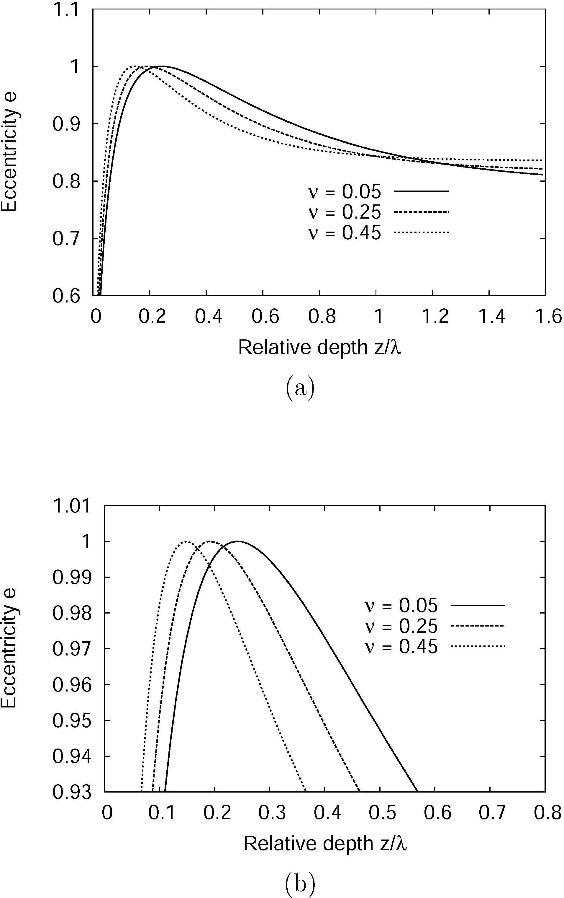
Using equation (B1), Figure B1 shows the particle motion eccentricity as a function of relative depth z/λ for different values of the Poisson’s ratio. The whole range of relative depth is displayed in Figure B1(a). Figure B1(b) shows a region in detail, where the particle motion changes from retrograde to prograde. This happens at a critical depth, z_C, when the vertical ellipse contracts in the horizontal direction; that is, U(z) = 0, which implies e = 1, and the particle motion displays a pure vertical locus. With the horizontal semi-axis contracting to zero, the resulting curve in theory would be a parabola which has e = 1. By checking the numbers of Figure B1(b) with a higher precision, we obtain that z_C = 0.2419λ for ν = 0.05, z_C = 0.1925λ for ν = 0.25, and z_C = 0.1482λ for ν = 0.45. One interesting feature is the fact that with normalization, the eccentricity is zero at the surface. This happens because both displacements U(z) and W(z) are normalized, implying that the geometrical locus is a circle, and e = 0 for a circle.

FIGURE B1
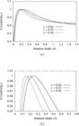
Normalized amplitudes eccentricity of the particle motion as a function of relative depth z/λ, for different values of the Poisson’s ratio: (a) the whole range of relative depth; (b) detail of the region where the particle motion changes from retrograde to prograde.

(2) The direction is given by ellipse’s derivative: if an ellipse has a retrograde motion, then Re[w(x, z, t)] increases with the increase of Re[u(x, z, t)]. Thus,

$$\frac{d\text{Re}[w(x,z,t)]}{d\text{Re}[u(x,z,t)]}>0.$$

On the other hand, if an ellipse has a prograde motion, the opposite happens; that is, Re[w(x, z, t)] decreases with the increase of Re[u(x, z, t)], and

$$\frac{d\text{Re}[w(x,z,t)]}{d\text{Re}[u(x,z,t)]}<0.$$

The derivative can be expressed as,

(B2) $${\displaystyle \frac{d\text{Re}[w(x,z,t)]}{d\text{Re}[u(x,z,t)]}}\approx {\displaystyle \frac{\mathrm{\Delta }\text{Re}[w(x,z,t)]}{\mathrm{\Delta }\text{Re}[u(x,z,t)]}}={\displaystyle \frac{\mathrm{\Delta }W(z)}{\mathrm{\Delta }U(z)}}{\displaystyle \frac{\cos (\omega t-kx)}{\sin (\omega t-kx)}}={\displaystyle \frac{\mathrm{\Delta }W(z)}{\mathrm{\Delta }U(z)}}\cot (\omega t-kx).$$

We do not need to consider the whole ellipse since we just want to check the direction at a given depth. We can compute numerically equation (B2), by calculating Re[w(x, z, t)] and Re[u(x, z, t)] in t₁ and t₂ = t₁ + Δt, for any horizontal distance x and a given depth z. If we consider just the first quadrant, the function cot⁡(ωt−kx) is always positive.

When U(z) and W(z) are both positive, then ΔW(z)/ΔU(z) is also positive, and the motion will be retrograde. On the other hand, when U(z) is negative and W(z) is positive, then ΔW(z)/ΔU(z) is negative, and the motion will be prograde.

Figure B2 shows the derivative expressed in equation (B2), numerically calculated, as a function of the relative critical depth z_c/λ. This scenario indicates the same values provides by the approach (1), that is, z_C = 0.24λ for ν = 0.05, z_C = 0.19λ for ν = 0.25, and z_C = 0.15λ for ν = 0.45.

FIGURE B2
Derivative ${\displaystyle \frac{d\text{Re}[w(x,z,t)]}{d\text{Re}[u(x,z,t)]}}$, numerically calculated, as a function of the relative critical depth z_c/λ.

(3) By making U(z) = 0 in the equation (56), we can find exactly the critical point for a given Poisson’s ratio ν:

$$A[e^{-qz}-2qs{(s^2+k^2)}^{-1}{e}^{-sz}]=0,$$

or

(B3) $$(s-q)z=\log [2qs{(s^2+k^2)}^{-1}].$$

Using the equations (59) and (60) in equation (B3), we obtain the expression:

(B4) $$\frac{z_C}{\lambda }=\frac{\log \left({\displaystyle \frac{2\sqrt{1-{\alpha }_1^2{\gamma }^2}\sqrt{1-{\gamma }^2}}{2-{\gamma }^2}}\right)}{2\pi (\sqrt{1-{\gamma }^2}-\sqrt{1-{\alpha }_1^2{\gamma }^2})}.$$

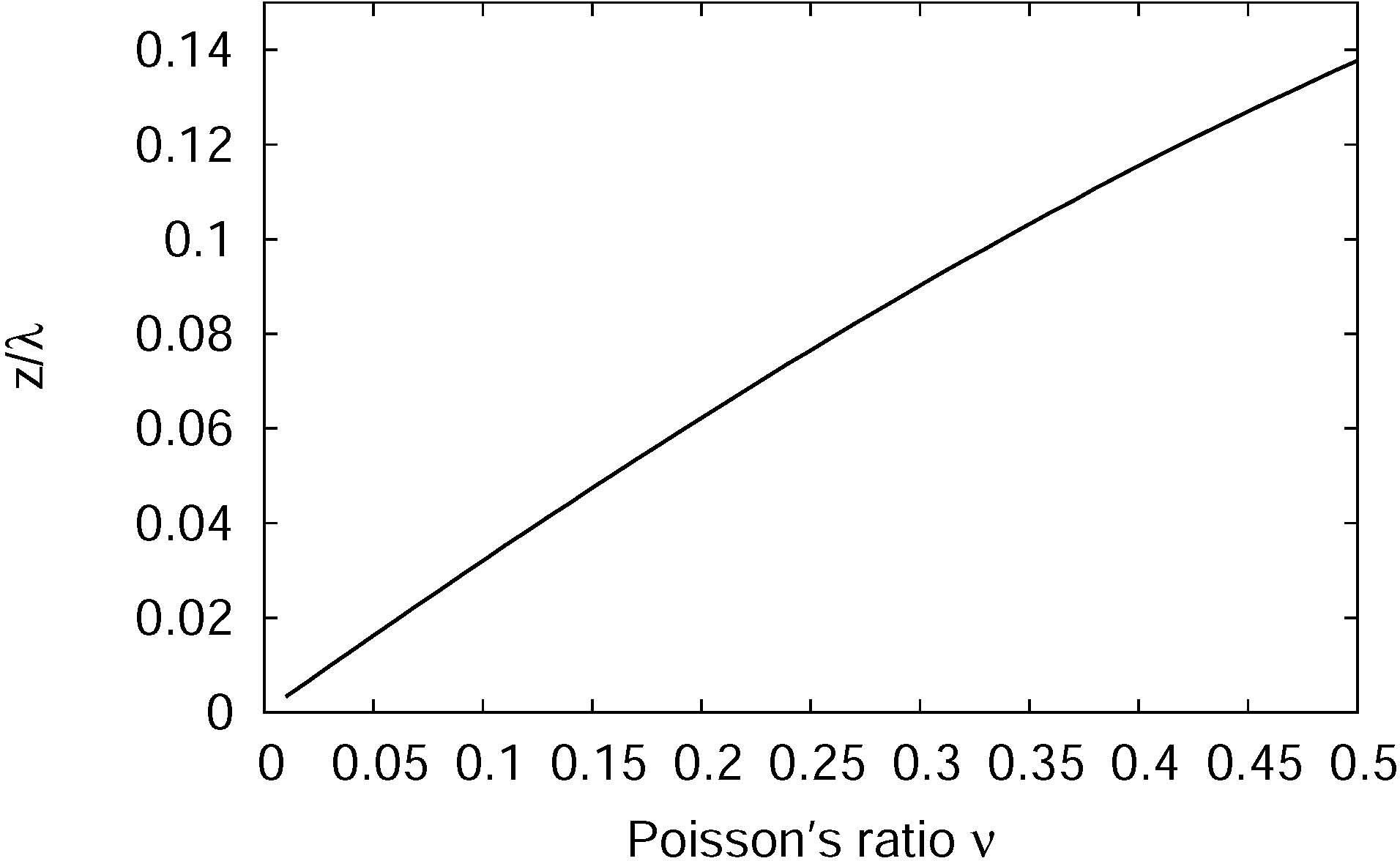
According to equation (B4), the relative critical depth z_c/λ depends on the root value γ² and on the parameter α₁. On its turn, γ² depends on α₁, and α₁ depends on ν. Figure B3 shows the critical depth z_c/λ as a function of ν. Notice that z_c/λ becomes shallower with the increase of ν.

FIGURE B3
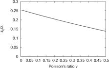
Relative critical depth z_c/λ as a function of ν. Notice that the critical depth becomes shallower with the increase of ν.

Notice that the critical depth z_C computed here corresponds to the change from positive to negative sign in the U(z) or normalized U(z) curves presented in Figure 6.

Appendix C: Ellipse Longest Semi-axis

There is a particular depth at which the ellipse has the longest vertical semi-axis; that is, it coincides with the maximum of function W(z). If we differentiate equation (58) in relation to z, we have the following:

$$\frac{dW(z)}{dz}=Aq[q{e}^{-qz}-2k^{2}s{(s^2+k^2)}^{-1}{e}^{-sz}].$$

Its maximum point is related to the condition dW(z)/dz = 0, which leads to:

(C1) $$(s-q)z=\log \left[\frac{2k^{2}s}{q(s^2+k^2)}\right].$$

Using the equations (59) and (60) in equation (C1), we have

(C2) $$\frac{z}{\lambda }=\frac{\log \left[{\displaystyle \frac{2\sqrt{1-{\gamma }^2}}{\sqrt{1-{\alpha }_1^2{\gamma }^2}(2-{\gamma }^2)}}\right]}{2\pi (\sqrt{1-{\gamma }^2}-\sqrt{1-{\alpha }_1^2{\gamma }^2})}.$$

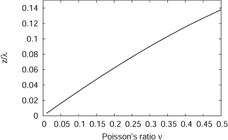
According to equation (C2), the relative depth z/λ (in which the ellipse has the longest semi-axis) depends on γ² and on α₁. Again, on its turn, γ² depends on α₁, and α₁ depends on ν. Figure C1 shows the variation of this relative depth z/λ as a ν function. Notice that this depth is usually shallow and becomes a little deeper with the increase of ν. Checking the numbers of Figure 15 with a higher precision, we have that z = 0.0162λ for ν = 0.05, z = 0.0765λ for ν = 0.25, and z = 0.1270λ for ν = 0.45. These values are consistent with the three maxima of Figure 7(a).

FIGURE C1
Relative depth z/λ in which the ellipse has the longest semi-axis, as a function of ν.

References

• ^[1] L. Rayleigh, Proceedings of the London Mathematical Society 17, 4 (1887).
• ^[2] M.A. Pelissier, H. Hoeber, N. van de Coevering and I. F. Jones (eds.), Classics of elastic wave theory (Society of Exploration Geophysicists, Tulsa, 2007).
• ^[3] H. Kolsky, Stress waves in solids (Dover Publications, New York, 1963).
• ^[4] L. Knopoff, Bulletin of the Seismological Society of America 42, 307 (1952).
• ^[5] W.M. Ewing, W.S. Jardetzky and F. Press, Elastic waves in layered media (McGraw-Hill, New York, 1957).
• ^[6] K.F. Graff, Wave motion in elastic solids (Dover Publications, New York, 1991).
• ^[7] J. Miklowitz, The theory of elastic waves and waveguides (North Holland, New York, 1978).
• ^[8] I.A. Viktorov, Rayleigh and Lamb waves: physical theory and applications (Plenum Press, New York, 1967).
• ^[9] J.D. Achenbach, Wave propagation in elastic solids (North Holland Pub., Amsterdam, 1984).
• ^[10] D. Royer, Ultrasonics 39, 223 (2001).
• ^[11] J.A. Hudson, The excitation and propagation of elastic waves (Cambridge University Press, Cambridge, 1980).
• ^[12] C.T. Schröder and W.R. Scott Jr., Journal of the Acoustical Society of America 110, 2867 (2001).
• ^[13] C.H. Chapman, Fundamentals of seismic wave propagation (Cambridge University Press, Cambridge, 2004).
• ^[14] S. Stein and M. Wysession, An introduction to seismology, earthquakes, and earth structure (Blackwell, Malden, 2003).
• ^[15] L.W. Griffiths, Introduction to the theory of equations (Wiley, Nova Iorque, 1947), 2 ed.
• ^[16] G. Birkhoff and S. Mac Lane, A survey of modern algebra (CRC Press, Boca Raton, 2010), 5 ed.

Publication Dates

• Publication in this collection
  06 Dec 2024
• Date of issue
  2024

History

• Received
  28 July 2024
• Reviewed
  07 Oct 2024
• Accepted
  23 Oct 2024