Stability and multi-population in a 3-state rock-paper-scissors game

Abstract

Statistical physics provides many tools to treat ecological models far from equilibrium. One of them, mean field theory, is appropriate as an initial step to a more realistic investigation of a complex system. In particular, Lotka-Volterra predator-prey system was one of the first strategies employed to study a biological community, and later, inspired and originated the rock-paper-scissors game. In this paper, the game is analysed in the context of the mean field theory, in the pair approximation and also through the Monte Carlo technique. The emphasis is on the stability condition and the number of species in the stationary regime. According to the pair approximation approach there are three possibilities concerning the kind of stability: marginal stability, asymptotic stability and instability, shown in a 1D and 2D phase diagram. Moreover, the rock-paper-scissors game in a lattice is studied via Monte Carlo simulations. The main achievements are coarsening in 1D and a 2D phase diagram indicating the edges between single species concentration and multi-population states.

Keywords:
Monte Carlo; Game Theory; Biodiversity

1. Introduction

This paper addresses an investigation of a model situated within the scope of evolutionary game theory (EGT). Evolutionary game theory is a conceptual structure employed in the study of the evolution of strategies in specific populations. The term ‘evolution’ is not to be intended as just mere biological evolution, but also cultural evolution in the social behavior among humans living in society. Strategies, here, mean the conduct of a group of individuals in any situation. The main interest is in the outcome of collective comportments on a particular strategy over time. An important notion in EGT is the idea of fitness; it is a measure of how adequate an individual is when compared with all others living in the same environment. It indicates the odds of a given organism to generate an offspring. The quantity in question relies on the interaction of an entity (be it a molecule or an animal) with the rest of the community members. Therefore, its value changes with time affecting the concentrations of the competing species. Usually (as in this paper), the fitness of a player in a population depends on its frequency, a situation known as frequency-dependent selection. Specifically, this contribution discusses a cyclic game in which a given agent is the victim and oppressor of different species.

In the first half of the twentieth century, the Lotka-Volterra predator-prey system [¹, ²] was a convenient framework to study the dynamics of the struggle for existence between different competitors. Usually this ecological model is described in terms of only two species, i.e., dominant and dominated. In the early stage, this approach was successful in providing estimates for macroscopic quantities such as the concentration of predators (or preys) in the stationary regime. This nonspatial game has given rise to a more elaborated model with cyclic dominance, namely the rock-paper-scissors (RPS) game with three or more distinct groups. Evolution in computer science has allowed the investigation of biological communities with spatially distributed individuals, in a closer similarity to actual ecological environments.

The literature on the rock-paper-scissors game is broad, concerning the model in its mixed version or in the stochastic description, with three or more different participants and intricate food webs [³,⁴,⁵,⁶]. This procedure is also relevant outside the biological context, extending from economics, where agents may be the diverse types of consumers, to game theory. Tainaka was one of the pioneers to analyse the cyclic RPS game in an extended lattice, with homogeneous transition rates [⁷]. He studied pattern formation as a consequence of spatial correlations. He discussed, in particular, the inadequacies of the mean field and the pair approximation techniques to describe the onset of strings and vortices. Another prominent work related to a cyclic Lotka-Volterra model in 1D was due to Krapivsky et al. [⁸, ⁹]. Formulating the dynamics of the agents in terms of moving interfaces, it was possible to obtain interesting effects such as coarsening. Strictly, these authors discovered a power law dependence for the average domain size with Monte Carlo steps. It is reasonable to expect in 1D, with three distinct players and uniform transition probabilities, that only one remaining group overcomes the whole lattice with equal chances, the other competitors leaving the game. Therefore, a major step, is to study the consequences of species-dependent transition rates on the survival probability in the asymptotic limit (t → ∞). A detailed investigation by Venkat et al. [¹⁰], analyses this situation in the one-dimensional ring with the possibility of mobility between distinct adjacent individuals. A rich phase diagram is obtained showing the diverse regions with the predominance of a given species. Indeed, they have found disobedience with the principle of the survival of the weakest [¹¹], at least in 1D.

Additional degrees of freedom, as in the 2D square lattice approach, may alter drastically qualitatively and quantitatively the properties of the game. In the first place, the chance of surviving in the stationary regime depends mainly on the transition rates instead of the initial distribution of the agents. There is a threshold for the species occupation number in a given dimension; if this limit is exceeded, the system is brought into a frozen state [¹²]. This number of possible distinct members increase with dimension. A treatment with more types of distinct groups permits a more precise examination of the intrinsic mechanisms related to phenomena such as coexistence; internal segregation and cooperation. Indeed, systems like the rock-paper-scissors model in a two-dimensional lattice exhibit long-range order, i.e., a regular spatial arrangement of the parts of a structure over large distances. This predictability of the game allows a more complete perception of pattern formations in 2D, such as rotating spirals.

There is strong evidence supporting the correspondence of the rock-paper-scissors game with real-world ecosystems. Specifically, examples of competing groups with cyclic dominance in nature are coral reef invertebrates [¹³] and lizard populations in California [¹⁴]. The motivation of this article is to exploit fully the effects of the random character of a numerical simulation on the kind of stability condition and therefore, to examine precisely the chances of all distinct individuals to exist together. It is worth noting that the treatment type has a great influence on the balance and consequently on the population of the final state.

The outline of the paper is as follows: in the next section, it is discussed the RPS model. The results of the analytical method are presented considering the model with both uniform and nonuniform invasion rates. To manage the shortcomings of the mean field treatment, it is introduced the pair approximation (PA) technique with special emphasis on the more general situation of nonhomogeneous transition rates. Moreover, through the Monte Carlo (MC) analysis the occurrence of order from disorder, roughening and diversity in 1D or 2D is observed. In the last section, it is summarized the main conclusions.

2. The Model

The popular rock-paper-scissors game well-known by kids worldwide became a relevant framework in game theory, a branch of biomathematical computation. The model and its generalized versions have gained the attention of numerous theoretical scientists due to the vast applicability in fields such as economics, ecology, strategy, and many more. It is usually convenient to study this game both from the analytical-collective standpoint (MFT or PA), i.e., via the concentrations of the agents or by the lattice-individual view (MC), with knowledge of the species type in each site. In the simplest case, each participant is a predator and prey of different species in such a way that members of the same group do not interact; they are inert. Schematically, the following reaction illustrates the dynamics:

(1) $$0\stackrel{{\alpha }_{01}}{\to }1\stackrel{{\alpha }_{12}}{\to }2\stackrel{{\alpha }_{20}}{\to }0$$

In the previous diagram, the quantities α_ij (i ≠ j) are transition rates, i.e., probabilities per time. For instance, one may normalize them through: α = α₀₁ + α₁₂ + α₂₀, and therefore by assuming α_ij = α_ij/α. It is important to realize that this definition implies rates being within the interval [0,1]. This strategy will be adopted in the rest of this paper. As a result, α_ij denotes the rate with which species i overcomes j.

The main ingredient sustaining biodiversity is the cyclic competition, as in the above description. In what follows, it will be shown that according to the analytical framework, the extinction is an event that never occurs, whereas in the structured scenario it may happen as a consequence of the finite size of the lattice.

3. The Results

3.1. Mean field analysis

The mean field approach to the RPS game is the appropriate starting point to get a qualitative view on the behavior of the ecosystem. In this framework, there is no spatial structure, and each species is conveniently described by its concentration, i.e., by the probability of being chosen at random, (P(0), P(1), P(2)). The reference to a single individual, whatever its species, is completely devoid of meaning. The set of coupled nonlinear differential equations (2) illustrates how a specific agent struggles for existence:

(2) $$\begin{array}{l}\dot{P}(0)=P(0)(+{\alpha }_{01}P(1)-{\alpha }_{02}P(2)),\hfill \\ \dot{P}(1)=P(1)(-{\alpha }_{10}P(0)+{\alpha }_{12}P(2)),\hfill \\ \dot{P}(2)=P(2)(+{\alpha }_{20}P(0)-{\alpha }_{21}P(1)),\hfill \end{array}$$

Above, the dots over the P ’s denote time derivatives. The system of equations (2), has three trivial equilibrium points. These points are absorbing states and correspond to the vertices of the state space, shown below.

(3) $$\begin{array}{l}P(0)=1,P(1)=0,P(2)=0,\\ P(0)=0,P(1)=1,P(2)=0,\\ P(0)=0,P(1)=0,P(2)=1.\end{array}$$

Moreover, it is worth noting that the trivial equilibrium points are independent of the nature of the transition rates, they are still a valid solution in the general case where there is no symmetry and all transition rates are different.

According to the stability analysis theory [¹⁵], the determination of the signs of the real part of the eigenvalues of the jacobian matrix (J) offer a direct criteria for the verification of the type of stability of the equilibrium points: asymptotically stable, marginally stable, or unstable. The eigenvalues of the matrix (4) should be calculated through the characteristic equation det(J − λI) = 0, where λ is an eigenvalue of the jacobian and I is the identity matrix. The principal motivation of this paper is to analyse the rock-paper-scissors game in the case of the symmetric solution (α_ij = α_ji, ∀i ≠ j), as a starting point. As a consequence, one obtains:

(4) $$J={\left[\begin{array}{ccc}\frac{\partial f_1}{\partial x_1}& \frac{\partial f_1}{\partial x_2}& \frac{\partial f_1}{\partial x_3}\\ \frac{\partial f_2}{\partial x_1}& \frac{\partial f_2}{\partial x_2}& \frac{\partial f_2}{\partial x_3}\\ \frac{\partial f_3}{\partial x_1}& \frac{\partial f_3}{\partial x_2}& \frac{\partial f_3}{\partial x_3}\end{array}\right]}_{P=\overline{P}}$$

where f_i stands for the nonlinear function dependence $\stackrel{.}{P}(i)$ upon the other species populations. Therefore, the eigenvalue equation reduces to:

(5) $$-{\lambda }^3-\lambda {({\alpha }_{02})}^2{P}_0{P}_2-\lambda {({\alpha }_{01})}^2{P}_0{P}_1-\lambda {({\alpha }_{12})}^2{P}_1{P}_2=0$$

3.1.1. Homogeneous case

Consider now a particular solution of the equation (5). The simplest case occurs when one has homogeneous transition rates, i.e., (α_ij = + 1,∀i ≠ j). In that context, the system (2) admits another equilibrium point (a central point), i.e., (P₀ = 1/3, P₁ = 1/3, P₃ = 1/3). By applying the uniform condition to the equation (5) one has the following eigenvalues:

$${\lambda }_1=0,{\lambda }_2=+i\frac{\sqrt{3}}{3},\mathrm{}{\lambda }_3=-i\frac{\sqrt{3}}{3}$$

By inspection of the above relations, it is possible to realize that the real parts of the eigenvalues are all equal to zero. Therefore, one may conclude that the middle point is marginally stable. The others, the trivial equilibrium points, the absorbing states (3), are unstable against invasions of their predators, and are stable against invasions of their preys. Graphically, in the (Figure 1), one may note the marginal stability of the central point, which is indicated by the three closed orbits around the middle point. Moreover, the symmetry of the curves is related to the uniform transition rates. Through a direct inspection of the system of equations (2) and a little algebra effort, it is also possible to derive two constants of the motion:

Figure 1
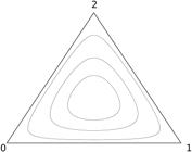
Ternary diagram: homogeneous transition rates. Each point represents a specific concentration in configuration space. The vertices correspond to the maximum species occupation.

(6) $$P(0)+P(1)+P(2)=\text{Constant 1},$$

and

(7) $$P(0)\cdot P(1)\cdot P(2)=\text{Constant 2}.$$

The above-mentioned equations (6) and (7) are valid expressions at any instant of time. In addition, the first relation implies that the total concentration of the different agents is constant through all times. However, this condition itself does not prevent one or more species from extinction. The statement present in the second equation implicitly contains the criteria that avoid elimination of any species. For instance, suppose that one group could eventually die out, leaving the game; then in this case, equation (7) is violated, i.e., its right side would vanish. Moreover, it is possible to observe from (Figure 1) that the motion in the state space is periodic and corresponds to an oscillatory movement without friction. The same conclusions apply equally well below in the heterogeneous case.

3.1.2. Heterogeneous case

The non-uniform approach to the set of equations (2) (α₀₁ ≠ α₁₂ ≠ α₂₀, and α_ij = α_ji,∀i ≠ j) permits the calculation of one more equilibrium point: $(\frac{{\alpha }_{12}}{\alpha },\frac{{\alpha }_{20}}{\alpha },\frac{{\alpha }_{10}}{\alpha })$, where α = α₀₁ + α₁₂ + α₂₀. Taking these conditions on the characteristic equation (5) one obtains the set of eigenvalues:

$${\lambda }_1=0,{\lambda }_2=+i\frac{\sqrt{{\alpha }_{01}{\alpha }_{12}{\alpha }_{02}\alpha }}{\alpha },{\lambda }_3=-i\frac{\sqrt{{\alpha }_{01}{\alpha }_{12}{\alpha }_{02}\alpha }}{\alpha }.$$

Note that one may conclude that the non-trivial equilibrium point is also marginally stable. It is shown in (Figure 2) that the orbits exhibit no symmetry, as expected due to the heterogeneous transition rates.

Figure 2
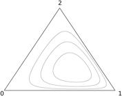
Ternary diagram: heterogeneous transition rates. As above, each point in configuration space is a possible state of the system.

Contrary to what one would expect, it is not the agents with the highest invasion rate that will overcome the ecosystem. Instead, the strongest individuals will only promote a reduction, with more efficiency, of their prey. As a result, there will be an enhancement in the population of the predators of the more competitive species. This phenomenon is best known as survival of the weakest. As above, in this case, one has two integrals of the motion:

(8) $$P(0)+P(1)+P(2)=\text{Constant 3}$$

and

(9) $$P{(0)}^{{\alpha }_{12}}\cdot P{(1)}^{{\alpha }_{02}}\cdot P{(2)}^{{\alpha }_{01}}=\text{Constant 4}$$

3.2. Pair approximation

The MFT technique provides only a brief overview of the characteristics of the RPS game. To attain a better understanding of the model, a refinement of the preceding equations (2) is required. For instance, consider the following set of master equations:

(10) $$\begin{array}{l}\dot{P}(0)=+{\alpha }_{01}P(0,1)-{\alpha }_{20}P(0,2),\\ \dot{P}(1)=-{\alpha }_{01}P(1,0)+{\alpha }_{12}P(1,2),\\ \dot{P}(2)=+{\alpha }_{20}P(2,1)-{\alpha }_{12}P(2,1),\end{array}$$

Above, the definitions of P(i)(i = 0, 1, 2) and $\stackrel{.}{P}(i)$ are analogous to the previous set of equations (2). The quantity P(i, j) denotes the probability of finding species i in a nearest neighbor site of species j. Each term P(i, j) in the previous equations (10) is dependent on sets of 3-tuple functions such as P(i, j, k). The definition of the probability P(i, j, k) is analogous to the definition of P(i, j): it is the probability of finding species i and k in the first neighborhood of j, not necessarily in the immediate vicinity of each other. The triplets P(i, j, k), in turn, show a dependence on the 4-tuple probabilities P(i, j, k, l), and this processes continues indefinitely. To circumvent the problem of solving endless interdependent sets of equations, one may adopt the pair approximation ansatz: P(i, j, k) = P(i, j) ⋅ P(j, k)/P(j). Therefore, this procedure yields a system of nine coupled nonlinear differential equations that is integrated with the fourth-order Runge-Kutta method.

(Figure 3) exhibits the results of the integration of the set of referred equations for the specific situation where: α₀₁ = α₁₂ = α₂₀ = 1. One may note by direct inspection of the graph (3) that the single species probabilities P(i) diverge in the asymptotic limit (t → + ∞), once in turn. In addition, (Figure 4) shows two phase diagrams in 1D (upper panel) and 2D (lower panel), indicating the distinct types of stability: instability (red), asymptotic stability (blue), and weak marginal stability (green). These results are a generalization of the work of Tainaka [⁷]. Strictly, the paper of Tainaka considers only one point in parameter space; rather than that, in this contribution, a slice of the phase space is covered.

Figure 3
It is shown the different probabilities for the unique populated states: P(0), P(1), P(2) as a function of time. These results represent a specific point in phase space: α₀₁ = α₁₂ = α₂₀ = 1.

Figure 4
Pair approximation phase diagrams. Upper panel: 1D. Lower panel: 2D. Different types of stability: instability (red), asymptotic stability (blue), and weak marginal stability (green). In both diagrams (1D or 2D), it is adopted α₀₁ = 0.45.

3.3. Monte Carlo

The Monte Carlo method was initially conceived to study ergodic systems, and its huge versatility stimulated the interest and curiosity of many researchers of different scientific lines including biology, economics, mathematics, statistics, and so on. For instance, the standard Monte Carlo technique may be employed in the evaluation of multi-dimensional integrals, is currently used to simulate solute diffusion in a lattice, to describe the dynamical evolution of molecules, in the investigation of biological systems, to name just a few examples.

In this contribution, the central point is to analyse the principal properties of the RPS game and its variants in a one-dimensional lattice as well as in the two-dimensional ring. In the structured version, the game reveals many surprising aspects that are not present in the analytical-collective description. As will be discussed below, among typical attributes of the model are extinction of one or more species, coarsening and domain growth in one dimension, and an asymptotic stability of the middle-point in the configuration space.

For that purpose, it was devised an algorithm to prepare the initial sample, to follow the trajectory of the system in the configuration space, and to determine all the relevant properties. In the first stage, the algorithm distributes the different agents on the lattice so that the probability of a given individual to attain a specific site is 1/3. In addition, in each MC update, the algorithm keeps all nearest neighbor sites with distinct species, in a strategy designated to improve the performance of the game. By selecting a predator-prey pair, the method is able to decide a possible event occurrence. If elimination takes place, the predator leaves an offspring on the adjacent site, and the defeated competitor goes away.

(Figure 5) shows two photographs of the model considered in this paper, on a two-dimensional square lattice. For instance, each color point represents one individual (0, 1, 2) in its site. Notice that, as time goes by, the system becomes self-organized. Regardless of the initial condition, the system always comes to the middle equilibrium point (1/3, 1/3, 1/3), as may be seen from (Figure 6). It is important to realize that stochastic fluctuations have major effects on small system sizes. For instance, the possibility of diversity loss grows as the lattice extension is reduced. Moreover, one may note that for larger grids, the stochastic noise decreases considerably, and for sufficient amounts of time the concentration of species j, P(j), approaches 1/3. More specifically, as one goes from small to greater lattices, the fluctuations of the domain areas around its average value drop, see (Figure 5). As a result, a convergence of the distinct species concentrations is achieved in finite times (Monte Carlo steps). A detailed discussion is presented in [⁷].

Figure 5
Monte Carlo two-dimensional simulations in the square lattice with N = 10,000; each color point represents one site. Higher panel: snapshot of the system with 1 Monte Carlo step. Inferior panel: snapshot of the system with 1000 Monte Carlo steps.

Figure 6
Monte Carlo 2D ternary diagram with symmetric transition rates. The initial state spirals into the middle point.

Therefore, one may conclude that the numerical analysis is consistent with an asymptotically stable central point, as opposed to the previous MF analytical solutions described above. It is interesting to appreciate that distinct approaches to the same RPS game model may lead to rather conflicting results. A possible argument to explain this unexpected property is that while the constant of the motion (6) is still valid, the other integral of the motion (7) is no longer reasonable in the context of the MC technique. The MC simulation exhibits a kind of damping effect with decreasing species concentration amplitudes over time.

A lot of intricate variants of the RPS game with more species and complex food webs have been proposed and studied via the Monte Carlo method by many authors. Surprisingly, it must be stressed that there is a threshold value for the biodiversity of an ecosystem, it depends on the dimension at hand, beyond that limit the system halts. Strictly, in an extended version of the RPS game with four kinds of players and with uniform transition rates (α_ij = 1, i ≠ j), comes about two pairs of mutually neutral competitors. In 1D or higher dimensions, couples of inert agents may prevail in the asymptotic limit (t → ∞).

For instance, in 1D the system organises into single-species domains of growing sizes with alternating prevalence of different groups with the same members. In the course of time, the average domain size grows up indefinitely until one or more groups of neutral competitors overcome the whole lattice, indicating the end of the game. A clever strategy to approach the game in 1D, is to formulate dynamical evolution in terms of adjacent interfaces between distinct sets of individuals. Below is exhibited schematically the reactions that describe the kinetics illustrated in (Figure 7):

Figure 7
Monte Carlo one-dimensional dynamics; the horizontal line indicates the different sites (L = 500), time flows in the upward vertical direction. Each color point or stripe represents a given species: 0, 1, 2, 3. Top panel: species 0 and 2 (or 1 and 3) are mutually inert, χ = 0.00, bottom panel: the neutral groups become slowing active, with transition rate χ = 0.01.

$$\begin{array}{c}0\to 1\to 2\to 3\to 0,\\ 0\underrightarrow{x}21\underrightarrow{x}3.\end{array}$$

Strictly, current progress may be accompanied through the pictures exhibited in Figures (7). These Figures represent the dynamical evolution of the RPS game in 1D. Time is oriented in the upward vertical direction, while each color site (black, blue, red, green) is associated with a given species type (0, 1, 2, 3) in the horizontal line. One may realize, by inspection of the left panel of (Figure 7), the existence of rigid walls between the “pairs” black-red (0–2) and blue-green (1–3). This is associated with the cooperative inert couples, with a null χ = 0.00. The neutral barriers become slow-moving interfaces in the case of χ = 0.01, note the small shift between the black-red and blue-green patners, see the right panel of (Figure 7).

(Figure 8) below shows a sketch of a portion of the 2D phase diagram of the rock-paper-scissors game. The dashed lines set the boundaries between single- and multi-population states. More specifically, the I and III locations indicate mono-concentrations with 99% of chance, and region II represents high diversity configurations.

Figure 8
Monte Carlo 2D phase diagram for N = 2500 lattice sites. Regions I and III indicate single-populated states, and region II indicates multiple species concentration. The dashed lines are the edges between mono- and multi-population locations. In this case it is adopted α₀₁ = 0.50.

4. Discussion and Conclusions

The principal purpose of this article was to investigate some properties of an ecological model with cyclic dominance both in the mixed-analytical case and in the stochastic-numerical situation as well. Despite the reduced amount of species and the nonphysical trait of symmetric interactions, the RPS game represents an initial departure to a more accurate examination of the intriguing relations among real living organisms. Familiar concepts to biologists such as extinction, survival of the fittest, and stability may be studied by resorting to the aforementioned model.

The fundamental task of statistical mechanics is to study the macroscopic properties of a system as a consequence of the microscopic model of the constituent parts that comprise a given structure, be it composed of living creatures or not. Therefore, as one may note via the previous Figures (5) and (7), spatial organization arises from the elementary hypothesis of cyclic competition among three or more entities. A minimal model of a predator-prey system with interactions mediated only through species concentrations is not adequate to investigate the diversity issue accurately. More specifically, one must undergo an extended lattice analysis that allows a major comprehension, with detailed knowledge, of the circumstances that favor a coexistence state.

Diversity loss in a biological community is a possible event that may occur in the MF and the PA scenarios; see [¹⁶] for a reference, but is more likely to be found in lattice-driven systems, due to the peculiar random character of such finite structures. For instance, stochastic effects are more pronounced in low spatial dimensions, i.e., in 1D the RPS game with three distinct competitors always evolves to a single populated state.

From a biological point of view, the reduction or harm in stability may be attributed to invasion of exotic species, unexpected scarcity of nutrients, climate changes, etc. The stability condition itself does not uniquely specify the state condition of the system in the long run, i.e., in the asymptotic regime (t → ∞). Strictly, the 2D MC simulation with symmetric interactions, as discussed above, is consistent with an asymptotically stable central point, a state with the highest species number; see (Figure 6). A similar scenario is encountered with non-uniform transition rates. In this last case, namely in the asymmetric context, a state with a single species population may be attainable in the stationary limit, with minimal diversity. The only requirement is just that one group dies out, which in turn, would give rise to the extinction of its predators. The same conclusion is no longer true in the mean field technique, where the marginal stability of the middle point yields the highest populated state; see Figures (1) and (2). Otherwise, in the pair approximation method the emergence of instability drives the system into an impoverished configuration, with a single group of individuals prevailing in the stationary limit, see (Figure 3).

Data Availability

The entire dataset supporting the results of this study has been made available on Kaggle and can be accessed at: https://www.kaggle.com/datasets/fbiopoderoso/figure-1-dataset.

References

• ^[1] A.J. Lotka, Proc. Nat. Acad. 6, 410 (1920).
• ^[2] V. Volterra, Proc. of the Edinburgh Math. Soc. (Series 2) 6, 4 (1939).
• ^[3] J. Hofbauer and K. Sigmund, Evolutionary Games and Population Dynamics (Cambridge University Press, Cambridge, 1998).
• ^[4] J. Friedman and J. Gore, Current Opinion in Systems Biology 1, 114 (1939).
• ^[5] A. Szolnoki, M. Mobilia, L.L. Jiang, B. Szczesny, A.M. Rucklidge and M. Perc, J. R. Soc. Interface 11, 1 (2014).
• ^[6] G. Szabo and G. Fath, arXiv:cond-mat/0607344 (2007).
• ^[7] K.I. Tainaka, J. Phys. Soc. Jpn. 57, 2588 (1988).
• ^[8] L. Frachebourg, P. Krapivsky and E. Ben Naim, Phys. Rev. Lett. 77, 2125 (1996).
• ^[9] L. Frachebourg, P.L. Krapivsky and E. Ben-Naim, Phys. Rev. E. 54, 6186 (1996).
• ^[10] S. Venkat and M. Pleimling, Phys. Rev. E. 81, 021917 (2010).
• ^[11] M. Frean and E.R. Abraham, Proc. R. Soc. Lond. B. 268, 1323 (2001).
• ^[12] L. Frachebourg and P.L. Krapivsky, J. Phys. A: Math. Gen. 31, L287 (1998).
• ^[13] L.W. Buss and J.B.C. Jackson, Am. Nat. 113, 223 (1979).
• ^[14] B. Sinervo and C.M. Lively, Nature 380, 240 (1996).
• ^[15] D.G. Luenberger, Introduction to Dynamic Systems: theory, models, and applications (Wiley, New Jersey, 1937).
• ^[16] A.F. Lutz, S. Risau-Gusman and J.J. Arenzon, J. Theor. Biol. 317, 286 (2013).

Edited by

• Editor-in-Chief:
  Marcello Ferreira https://orcid.org/0000-0003-4945-3169

Publication Dates

• Publication in this collection
  11 July 2025
• Date of issue
  2025

History

• Received
  19 Nov 2024
• Reviewed
  21 Feb 2025
• Accepted
  16 Apr 2025