A comprehensive overview of the Young-Laplace equation

Uma revisão abrangente sobre a equação de Young-Laplace

Abstract

The Young–Laplace equation relates the pressure difference across a fluid interface to its curvature and surface tension and plays a fundamental role in physical phenomena and engineering applications. This work aims to present a clear and pedagogically oriented exposition of the physical and mathematical foundations of the Young–Laplace equation. The approach combines a theoretical derivation with illustrative examples based on common physical situations. The results demonstrate how the equation quantitatively explains pressure variations in curved interfaces and clarifies the role of curvature in determining equilibrium configurations. These examples highlight the consistency between the mathematical formulation and observable phenomena. By systematically linking theory, derivation, and application, the work provides an accessible and comprehensive reference that supports the teaching and learning at undergraduate and graduate levels.

Keywords:
Young-Laplace Equation; surface tension; surface curvature

Resumo

A equação de Young-Laplace relaciona a diferença de pressão através da interface de um fluido com sua curvatura e tensão superficial, desempenhando um papel fundamental em fenômenos físicos e aplicações em engenharia. Este trabalho visa apresentar uma exposição clara e pedagogicamente orientada dos fundamentos físicos e matemáticos da equação de Young-Laplace. A abordagem combina uma derivação teórica com exemplos ilustrativos baseados em situações físicas comuns. Os resultados demonstram como a equação explica quantitativamente as variações de pressão em interfaces curvas e esclarece o papel da curvatura na determinação das configurações de equilíbrio. Esses exemplos destacam a consistência entre a formulação matemática e os fenômenos observáveis. Ao conectar sistematicamente teoria, derivação e aplicação, o trabalho fornece uma referência acessível e abrangente para o ensino e a aprendizagem nos níveis de graduação e pós-graduação.

Palavras-chave:
Equação de Young-Laplace; tensão superficial; curvatura de superfície

1. Introduction

Interfaces are surfaces that separate two media from one another. Considering the solid, liquid, and gaseous phases, three primary types of interfaces can be readily identified: liquid-solid, liquid-gas, and solid-gas. Additionally, liquid-liquid interfaces occur between immiscible liquids, and solid-solid interfaces separate two different solid phases. The latter plays a crucial role in determining the mechanical, electrical, and thermal properties of composite solid materials. Gas-gas interfaces, on the other hand, represent regions where two gases meet and interact. However, this concept is particularly complex and challenging to study experimentally, as gas mixtures tend to occur very rapidly and are difficult to control.

In general, the term capillarity is used to describe phenomena that occur at liquid-liquid, liquid-gas, and liquid-solid interfaces. In such systems, interfaces are free to deform in order to minimize surface energy and achieve mechanical equilibrium. The Young-Laplace Equation (YLE) relates the pressure difference across an interface to its curvature and surface tension. This equation is the result of Thomas Young’s physical insight, combined with the mathematical formalism developed by Pierre-Simon Laplace.

Thomas Young laid the foundations for the equation in 1805 [¹], when he qualitatively described the principles governing certain aspects of fluid behavior. In the same year, Laplace developed a formal mathematical treatment representing Young’s ideas [²]. Laplace also incorporated earlier contributions from Francis Hauksbee and Johann Andreas Segner, who had proposed that capillary rise was caused by attractive forces between solids and liquids [³], and that liquids are held together by cohesive forces acting over very short distances – too short to be measured directly [⁴]. A detailed historical account of the development of capillarity theory, from Newton through Young and Laplace, can be found in ref. [⁵].

Despite its fundamental role in physics and engineering with practical applications across fields such as microfluidics, biotechnology, and geosciences, the YLE is almost entirely absent from undergraduate curricula. In fact, it is not covered, or even mentioned, in most current introductory physics textbooks. At present, the YLE appears only in advanced and specialized literature. Among the classical references are [⁶, ⁷, ⁸, ⁹, ¹⁰], while more recent sources include refs. [¹¹] and [¹²]. Introductory physics education studies that address the YLE in an accessible manner include refs. [¹³], [¹⁴] and [¹⁵].

This work aims to provide a coherent and accessible description of the YLE, including its physical foundations and mathematical formulation. All examples presented are based on easily observable phenomena and serve to illustrate the explanatory power of the YLE in understanding everyday occurrences. This text is not intended as a historical review, a mathematically rigorous derivation, or an exhaustive survey of current research. Rather, it is a compendium of principles and illustrative applications that may serve as educational material for classrooms, teaching laboratories, and other academic settings, making the YLE accessible and comprehensible for undergraduate and graduate students.

2. The Physical Origins and Consequences of Surface Tension

Condensed states of matter arise when the attractive (cohesive) forces between particles exceed the energy associated with their thermal motion. In the case of liquids, this results in a state that is denser and more cohesive than the gas phase, while remaining disordered. Liquids can generally be treated as continuous media and are characterized by macroscopic properties such as density, viscosity, and cohesive energy. Interfaces, such as liquid–liquid, liquid–gas, or liquid-solid, are characterized by a surface energy (or surface tension), which is defined as the excess free energy per unit interfacial area. Surface tension, on the other hand, is the tensile force per unit length acting along the interface. These two descriptions are dimensionally equivalent and conceptually consistent, stemming from complementary theoretical approaches and experimental observations.

The intermolecular interactions responsible for cohesive energy originate from electromagnetic forces and include direct Coulomb interactions between charges, charge–dipole interactions, dipole–dipole interactions, van der Waals interactions, among others. A detailed treatment of these interactions is provided in ref. [¹⁶]. Despite the diversity of specific mechanisms, intermolecular potentials generally share a characteristic form, as illustrated in Fig. 1a. This form features a steep short-range repulsive component, which prevents molecular overlap, and a weaker long-range attractive component. Together, these contributions produce a potential well centered around an equilibrium separation $r_e$, which determines the typical interparticle distance in the liquid and can be used to define an effective molecular diameter.

Figure 1
(a) Typical interaction potential $V\left(r\right)$ and resulting force $F\left(r\right)=-dV/dr$ between two atoms or molecules. At the equilibrium distance $r_e$, the energy is minimal and the force is zero. At distance $r_s$, the pair can be separated by a force $F_{max}$. The range $R$ of the potential is the maximum distance at which intermolecular forces are effective. (b) Schematic illustration showing two specific molecules (black dots), one inside the liquid and the other near the interface with a gas. The surface molecule has roughly half the number of neighbors (gray dots) compared to the interior molecule. This causes the molecules at the interface to be pulled inward, which creates internal pressure and forces the surfaces of liquid portions to contract until reaching a minimal area. (c) Density profile at the surface of the liquid with a gradual transition from the liquid density $\rho$ to the gas density.

Due to their high density, molecules in liquids interact with many neighbors located within the spatial range of the interaction potential (see Fig. 1b). These interactions define the cohesive energy of the liquid. In the bulk, molecules are symmetrically surrounded, and the net force on each averages zero. However, molecules near the surface experience an imbalance, with approximately half as many neighbors as in the bulk. As a result, interfacial molecules are pulled inward, generating an internal pressure and a restoring force that tends to minimize the surface area. Additionally, a lateral force arises at the liquid–gas interface, leading to a surface tension that acts parallel to the interface. This tension causes the surface to behave like an elastic membrane, resisting deformation. Consequently, although liquids flow readily, they are capable of maintaining highly stable shapes.

If the cohesive energy per molecule in the bulk of a liquid is denoted by $E$, at the liquid–gas interface, this energy is reduced to approximately $E/2$. Surface tension, $\gamma$, is a direct measure of this energetic deficit per unit area. Assuming an effective molecular diameter $r_e$, it follows that $\gamma \approx E/2r_e^2$, indicating a direct dependence on cohesive energy [¹⁰]. Table 1 summarizes the surface tension, density, boiling point, and vapor pressure for a selection of liquids. For substances where intermolecular forces are purely van der Waals in nature, $E\approx kT$ and $\gamma \approx 20$ mJ/m² at $T=25{,}^{\circ }$C. In contrast, polar molecules experience stronger intermolecular attractions, leading to higher cohesive energies, elevated boiling points, and greater surface tensions. For example, water exhibits $\gamma \approx 72$ mJ/m² due to its permanent dipole moment and hydrogen bonding. Mercury, a liquid metal characterized by strong metallic bonding, has a significantly higher surface tension of approximately $\gamma \approx 500$ mJ/m².

Table 1
Physical properties of some common liquids [¹⁰, ¹²].

	Surface tension (mJ/m2)	Boiling point (°C)	Density (kg/m3)	Vapor pressure (kPa)
Water (25°)	72	100	997	3.1
Water (100°)	58	100	972	101
Ethanol	22	78	789	6.1
Glycerol	64	290	1260	< 10−4
Mercury	485	357	13540	< 2 × 10−4

Molecules in a liquid undergo thermal motion, leading to continuous changes in their relative positions. Under such conditions, the appropriate energy to consider is the free energy, which accounts for the effect of random thermal motion via entropy, rather than solely the binding energy, as suggested by the simplified model described above [¹²]. At a liquid surface, capillary waves [⁷] can be thermally activated in a manner analogous to phonons in a crystal. Consequently, the surface energy of liquids typically decreases with increasing temperature. Moreover, thermal agitation prevents the interface from being sharply defined as a boundary separating the liquid and vapor densities. A more accurate description treats the interface as a finite transition zone, where the liquid density gradually decreases to match that of the surrounding vapor, as depicted in Fig. 1c. In this refined model, surface tension arises from the density gradient within the transition zone. This occurs because, as the density decreases, the average intermolecular separation increases. For separations slightly greater than the equilibrium distance $r_e$, but still within the range of the interaction potential, the molecules experience an attractive force (see Fig. 1a). This force acts along the density gradient at the interface, leading to a reduction in surface area and an increase in internal pressure.

The reasoning described so far for liquid–gas interfaces can be extended to the interface between two different liquids. Consider the interface illustrated in Fig. 1b, which separates two liquids, A and B. If the liquids do not mix, the molecules of A and B are more strongly attracted to their own kind than to the other species. As a result, molecules near the interface, on both sides, have fewer neighboring molecules of the same kind compared to those in the bulk. This leads to an excess energy per unit area at the interface, defined as the interfacial tension ${\gamma }_{AB}$. On the other hand, if molecules of A and B are more strongly attracted to each other than to themselves, the system spontaneously emulsifies and eventually mixes on a molecular scale. In a similar way, the concept of interfacial energy and tension can be extended to liquid-solid and solid–gas interfaces [¹⁰].

Although its origin can be explained at the molecular level, it is convenient to define surface tension on a macroscopic scale. It is easy to observe that work must be done in order to increase the area of an interface, such as blowing soap bubbles in air or injecting air bubbles into water. Suppose one intends to increase the interfacial area by an amount $\mathrm{\Delta }A$. The work $W_A$ required to achieve this increase must be proportional to the number of molecules that need to be brought to the surface, which, in turn, is proportional to $\mathrm{\Delta }A$. Surface tension is defined as the proportionality constant between $W_A$ and $\mathrm{\Delta }A$, that is,

(1) $$W_A=\gamma \mathrm{\Delta }A.$$

In other words, $\gamma$ represents the amount of energy that must be supplied to increase the surface area by one unit.

Consider the example of a water droplet in air. In the absence of gravity and other external fields, the spherical shape with radius $R$ corresponds to the configuration with the lowest surface energy [¹⁷]. The total work required to increase the area of the droplet by $\mathrm{\Delta }A$ is given by

(2) $$W=W_V+W_A.$$

The first term on the right-hand side of Eq. 2 refers to the work associated with the change in volume, defined as $W_V=-P\mathrm{\Delta }V-P_0\mathrm{\Delta }{V}_0$, where $P$ and $P_0$ are the pressures inside and outside the droplet, respectively. $\mathrm{\Delta }V$ and $\mathrm{\Delta }{V}_0=-\mathrm{\Delta }V$ represent the volume variations inside and outside the droplet, respectively. The second term on the right-hand side of Eq. 2 corresponds to the work associated with the change in surface area of the droplet, as defined in Eq. 1. In these terms, Eq. 2 can be rewritten as

(3) $$W=\left(-\mathrm{\Delta }P+\gamma \frac{\mathrm{\Delta }A}{\mathrm{\Delta }V}\right)\mathrm{\Delta }V,$$

where $\mathrm{\Delta }P=P-P_0$. The condition for mechanical equilibrium ($W=0$) leads to the relation

(4) $$\mathrm{\Delta }P=\gamma \frac{\mathrm{\Delta }A}{\mathrm{\Delta }V}.$$

In the case of a spherical droplet with an initial radius $R$ and a final radius of $R+\mathrm{\Delta }R$, we have that $\mathrm{\Delta }V=4\pi R^2\mathrm{\Delta }R$ and $\mathrm{\Delta }A=8\pi R\mathrm{\Delta }R$. Therefore,

(5) $$\mathrm{\Delta }P=\frac{2\gamma }{R}.$$

For a cylinder with an initial radius $R$, a final radius of $R+\mathrm{\Delta }R$, and constant length $L$, we obtain that $\mathrm{\Delta }V=2\pi LR\mathrm{\Delta }R$ and $\mathrm{\Delta }A=2\pi L\mathrm{\Delta }R$. Therefore,

(6) $$\mathrm{\Delta }P=\frac{\gamma }{R}.$$

Eqs. 5 and 6 are special cases of a more general relationship between pressure and curvature, defined by

(7) $$\mathrm{\Delta }P=2\gamma \kappa =\gamma \left(\frac{1}{R_1}+\frac{1}{R_2}\right),$$

which is denoted as the Young-Laplace Equation (YLE). In this equation, $\mathrm{\Delta }P$ is often denoted as Laplace pressure or pressure jump, and $\kappa$ is the mean curvature of the surface expressed in terms of the principal radii of curvature $R_1$ and $R_2$. Note that, in the case of a spherical droplet, $R=R_1=R_2$, and the Eq. 7 reduces to Eq. 5. In the case of a cylinder, $R=R_1$, $R_2=\infty$, and the Eq. 7 reduces to Eq. 6. In the case of a plane, $R_1=R_2=\infty$, and therefore $\mathrm{\Delta }P$ must equal zero.

Equation 7 not only explains the pressure difference across a liquid boundary but also asserts that the curvature $\kappa$ of liquid interfaces at mechanical equilibrium, without external forces, must remain constant across the entire interface. A variation in curvature at any spot on the interface would induce pressure variations, consequently causing fluid motion. This movement would persist until the pressure inequalities are resolved completely, resulting in a terminal state with uniform $\kappa$ across the interface.

3. Curvature

Curvature provides a measure of how much a curve deviates from a straight line or a surface deviates from a plane. In other words, it quantifies the rate at which a curve’s direction changes at a particular point. The expression in parentheses in Eq. 7 indicates that the curvature at any point on a smooth surface or curve can be defined in terms of two radii of curvature, located in two normal planes that intersect the surface along two principal curvature sections. These two normal planes are also orthogonal to each other, and their line of intersection defines the direction of the surface normal vector at the chosen point [¹⁴].

Figure 2 presents an illustration of how the curvature at a given point on a surface can be determined in terms of the radii of curvature. The curvature at a point $Q$ on the surface of a light bulb is determined by first identifying the direction of the vector $\overrightarrow{n}$ normal to the surface. The bulb is then sectioned along two mutually orthogonal planes (a red plane, parallel to the page, and a blue plane, perpendicular to the page) that intersect along $\overrightarrow{n}$. The intersections of these planes with the bulb’s surface define two curves whose radii of curvature at point $Q$ are denoted by $R_1$ and $R_2$. Each radius is that of a circle tangent to the corresponding curve at the point involved. These radii are treated as algebraic quantities according to the convention that $R$ is positive if the center of the corresponding circle lies inside the bulb, and negative otherwise. If there exists a symmetry axis (the $z$-axis in Fig. 2), and one of the two planes contains this axis (the red plane in Fig. 2), then $R_1$ and $R_2$ are referred to as the principal radii of curvature.

Figure 2
A light bulb is an example of a surface of revolution generated by the rotation of the planar curve $z=f\left(x\right)$ around the $z$-axis. In this example, the bulb is sectioned along two mutually orthogonal planes (red plane, parallel to the page, and blue plane, perpendicular to the page) that intersect along the vector $\overrightarrow{n}$, which is normal to the surface. The intersections of these planes with the surface of the bulb define two curves, whose radii of curvature at point Q are denoted by $R_1$ and $R_2$. These radii are treated as algebraic quantities according to the convention that $R$ is positive if the center of the corresponding circle lies inside the bulb, and negative otherwise.

3.1. The curvature of surfaces of revolution

In practice, the YLE in the form of Eq. 7 is useful and immediately applicable only to surfaces with explicit radii of curvature, e.g., planes, cylinders, and spheres. In cases involving surfaces with no explicit symmetries, non-differentiable surfaces, or surfaces defined in high-dimensional spaces, the calculation and even the concept of curvature can be more complex [¹⁸, ¹⁹]. Therefore, deriving a general expression for calculating the curvature of any surface is beyond the scope of this work. However, most physical systems with an interface between liquids and gases present a surface of revolution, which is a surface generated by rotating a planar curve around an axis located in the same plane as the curve. The bulb shown in Fig. 2 is an example of a surface of revolution, generated by rotating the planar curve $z=f\left(x\right)$ around the $z$-axis. For such cases, it is relatively easy to obtain explicit expressions for $R_1$ and $R_2$[¹⁰, ⁹].

According to Fig. 2, if $l$ is the curvilinear coordinate along the meridian curve of the bulb, oriented from bottom to top, and $\theta$ is the angle between the normal vector $\overrightarrow{n}$ to the curve and the $x$-axis, then $dl=-R_{1}d\theta$ and $x=R_2\cos \theta$, so that the mean curvature appearing in Eq. 7 can be rewritten as

(8) $$\kappa =\frac{1}{\text{2}}\left(\frac{1}{R_1}+\frac{1}{R_2}\right)=\frac{1}{\text{2}}\left(-\frac{d\theta }{dl}+\frac{\cos \theta }{x}\right).$$

Along the curve $f\left(x\right)$, $dx=dl\sin \theta$, $dz=dl\cos \theta$ and $dl={\left(d{x}^2+d{z}^2\right)}^{1/2}$. Using the notation $z^{\prime }=dz/dx$ and $z^{\prime \prime }=d^{2}z/d{x}^2$, it is possible to express that

(9) $$\cos \theta =\frac{dz}{dl}=\frac{dz}{dx}\frac{dx}{dl}=\frac{z^{\prime }}{{\left(1+z^{\prime 2}\right)}^{1/2}},$$

and

(10) $$\frac{d\theta }{dl}=\frac{d\theta }{dx}\frac{dx}{dl}=\frac{1}{{\left(1+z^{\prime 2}\right)}^{1/2}}\frac{d\theta }{dx}.$$

Additionally, considering that

(11) $$z^{\prime }=\frac{dz}{dx}=\cot \theta$$

and

(12) $$z^{\prime \prime }=\frac{d{z}^{\prime }}{dx}=\frac{d}{dx}\cot \theta =-\left(1+{\cot }^2\theta \right)\frac{d\theta }{dx},$$

one obtains

(13) $$\frac{d\theta }{dx}=-\frac{z^{\prime \prime }}{1+z^{\prime 2}}.$$

Substituting Eqs. 13, 10, and 9 into Eq. 8 results in the expression for the mean curvature as a function of the planar curve that generates the surface of revolution, that is,

(14) $$\kappa =\frac{1}{\text{2}}\left(\frac{z^{\prime \prime }}{{\left(1+z^{\prime 2}\right)}^{3/2}}+\frac{z^{\prime }}{x{\left(1+z^{\prime 2}\right)}^{1/2}}\right).$$

In deriving Eq. 14, a surface generated by rotating the planar curve $z=f\left(x\right)$ around the $z$-axis was considered. Let $g$ be the inverse function of $f$, that is, $x=g\left(z\right)=g\left(f\left(x\right)\right)$. Then, $z^{\prime }=1/\dot{x}$ and $z^{\prime \prime }=-\ddot{x}/{\dot{x}}^3$ (where $\dot{x}=dx/dz$ and $\ddot{x}=d^{2}x/d{z}^2$). Using these relationships, Eq. 14 can alternatively be written as

(15) $$\kappa =\frac{1}{\text{2}}\left(-\frac{\ddot{x}}{{\left(1+{\dot{x}}^2\right)}^{3/2}}+\frac{1}{x{\left(1+{\dot{x}}^2\right)}^{1/2}}\right).$$

3.2. Minimal surfaces

Surfaces with identically zero mean curvature are of particular interest. They arise, for instance, as solutions of Eq. 15 in the case $\kappa =0$. In this case, this equation takes the form

(16) $$x\ddot{x}-{\dot{x}}^2=1,$$

with solutions depending on the imposed boundary conditions. Equation 16 follows directly from the analysis of surfaces of revolution with zero mean curvature, which, as will be shown below, correspond to surfaces that locally minimize area, known as minimal surfaces.

The area of a surface of revolution generated by the rotation of the plane curve $x=g\left(z\right)$, with $-b\le z\le b$, is given by the functional

(17) $$A=2\pi \int x\mathit{d}l=2\pi {\int }_{-b}^{+b}x{\left(1+{\dot{x}}^2\right)}^{1/2}\mathit{d}z.$$

We can employ variational calculus to determine the differential equation that must be satisfied by a minimal surface. In order to do that, we set the variation $\delta A$, computed with respect to the variation $\delta x$, equal to zero, that is,

(18) $$\delta A={\int }_{-b}^{+b}{\left(1+{\dot{x}}^2\right)}^{1/2}\delta x\mathit{d}z+{\int }_{-b}^{+b}\frac{x\dot{x}}{{\left(1+{\dot{x}}^2\right)}^{1/2}}\delta \dot{x}\mathit{d}z=0.$$

Noting that $\delta \dot{x}=\delta dx/dz=d\delta x/dz$, and integrating the second term by parts, we obtain

(19) $$\begin{array}{ll}\delta A=\hfill & {\displaystyle {\int }_{-b}^{+b}\left[{\left(1+{\dot{x}}^{.2}\right)}^{1/2}-\frac{\left(1+{\dot{x}}^{.2}\right)\left({\dot{x}}^{.2}+x\ddot{x}\right)-x{\dot{x}}^{.2}\ddot{x}}{{\left(1+{\dot{x}}^{.2}\right)}^{3/2}}\right]}\hfill \\ \hfill & \times \delta xdz+\frac{x\dot{x}}{{\left(1+{\dot{x}}^{.2}\right)}^{1/2}}\delta x|{}_{-b}^{+b}=0.\hfill \end{array}$$

Taking into account the boundary conditions ($\delta x=0$ em $z=\pm b$) and the fact that the integral must vanish for any variation $\delta x$, the expression within brackets must be zero, resulting, therefore, in Eq. 16.

3.3. Examples

Equations 14 and 15 can be tested in some simple cases where the curvature values are known.

The surface of a sphere can be generated by rotating a circle whose equation is $x^2+z^2=R^2$. Considering the planar curve $x={\left(R^2-z^2\right)}^{1/2}$, we obtain $\dot{x}=-z{\left(R^2-z^2\right)}^{-1/2}$ and $\ddot{x}=-R^2{\left(R^2-z^2\right)}^{-3/2}$. Substituting these expressions into Eq. 15, we obtain the expected value for the mean curvature of a sphere, that is,

(20) $$\kappa =\frac{1}{\text{2}}\left(\frac{1}{R}+\frac{1}{R}\right)=\frac{1}{R}.$$

A cone can be generated by rotating the straight line $z=\alpha \left(x-R\right)$, for which $z^{\prime }=\alpha$ and $z^{\prime \prime }=0$. Substituting these expressions into Eq. 14, we find that the mean curvature of the cone, excluding the apex, is

(21) $$\kappa =\frac{1}{\text{2}}\left(0+\frac{1}{\left(R+z/\alpha \right){\left(1+1/{\alpha }^2\right)}^{1/2}}\right).$$

The curvature of a cylinder of radius $R$ is obtained by the limit $\alpha \to \infty$, yielding

(22) $$\kappa =\frac{1}{2R}.$$

Since planes can be defined by a constant value of $z$, they have zero curvature. The catenoid is another example of a minimal surface, which can be generated by the rotation of a catenary [²⁰, ²¹] defined by the planar curve

(23) $$x\left(z\right)=a\mathrm{}\cosh \left(z/a\right).$$

Substituting $\dot{x}=\sinh \left(z/a\right)$ and $\ddot{x}=\cosh \left(z/a\right)/a$ into Eq. 15, we find that the mean curvature of the catenoid is

(24) $$\kappa =\frac{1}{\text{2}}\left(-\frac{1}{a\mathrm{}{\cosh }^2\left(z/a\right)}+\frac{1}{a\mathrm{}{\cosh }^2\left(z/a\right)}\right)=0.$$

Equivalently, it is easy to verify that Eq. 23 satisfies Eq. 16, which in this case reduces to the fundamental hyperbolic identity ${\cosh }^2\left(z/a\right)-{\sinh }^2\left(z/a\right)=1$. That is, both the plane and the catenoid are minimal surfaces.

4. Derivations of the Young-Laplace Equation

From a physical perspective, the YLE can be derived through the force equilibrium [⁸] and thermodynamic equilibrium [⁷].

4.1 Force equilibrium

Figure 3 illustrates the surroundings of a point Q on a given surface. A circle of radius $r$ is drawn around it, defining the edges of a cap. The two principal curvature sections, labeled AB and CD, are drawn through Q, characterized by the radii $R_1$ and $R_2$, respectively. The presence of surface tension causes an infinitesimal length element $dl$ on the edge of the cap, located at point A for example, to be subjected to a force

(25) $$dF=\gamma dl.$$

Figure 3
Diagram used in the deduction of the Young-Laplace equation by the force equilibrium method.

The origin of this force can be understood as follows. According to Eq. 1, the work required to increase the area of the cap shown in Figure 3 by an infinitesimal amount $dA$ is given by

(26) $$d{W}_A=\gamma dA=\gamma dldr=dFdr,$$

where $dF=\gamma dl$ is the tension acting at the interface.

For a small angle ${\theta }_1$, the projection of this force along the direction of the normal vector $\overrightarrow{n}$ is given by $dF\sin {\theta }_1\approx dF{\theta }_1\approx \gamma dlr/R_1$. Considering four elements $dl$ at points A, B, C, and D, the resultant force along the normal $\overrightarrow{n}$ is given by

(27) $$d{F}_n=2\gamma \left(\frac{1}{R_1}+\frac{1}{R_2}\right)rdl.$$

This expression is independent of the choice of AB and CD and can therefore be integrated along the circumference that defines the edges of the cap. Since two orthogonal pairs have been considered, the integration over $dl=rd\varphi$ must be performed over a quarter of a revolution, resulting in

(28) $$\begin{array}{ll}{F}_n\hfill & ={\displaystyle \int d{F}_n}=2\gamma \left(\frac{1}{R_1}+\frac{1}{R_2}\right){\displaystyle {\int }_0^{\pi /2}{r}^{2}d\varphi }\hfill \\ \hfill & =\gamma \left(\frac{1}{R_1}+\frac{1}{R_2}\right)\pi r^2.\hfill \end{array}$$

The force on the cap caused by a pressure difference $\mathrm{\Delta }P$ across the surface is given by

(29) $$F_P=\mathrm{\Delta }PA=\mathrm{\Delta }P\pi r^2.$$

The YLE results from the equilibrium imposed by the equality $F_n=F_P$.

4.2. Thermodynamic equilibrium

Figure 4 illustrates the transformation of the infinitesimal area element $dA$ of a given surface. This transformation results from the volume variation $\mathrm{\Delta }V=\mathrm{\Delta }R\int \mathit{d}A$ and the area variation $\mathrm{\Delta }A=\int \mathit{d}{A}^{\prime }-\int \mathit{d}A$. The total work associated with this transformation is given by the sum

(30) $$W=W_V+W_A,$$

Figure 4
Diagram used in the deduction of the Young-Laplace equation by the energy method.

where

(31) $$W_V=-\mathrm{\Delta }P\mathrm{\Delta }V=-\int \mathrm{\Delta }P\mathrm{\Delta }R\mathit{d}A$$

is the work associated with the volume variation, and

(32) $$W_A=\gamma \mathrm{\Delta }A$$

is the work associated with the area variation.

According to Fig. 4, the surface areas before and after the transformation, $dA$ and $d{A}^{\prime }$, respectively, can be expressed as $dA=d{l}_{1}d{l}_2$ and $d{A}^{\prime }=d{l}_1^{\prime }d{l}_2^{\prime }$, where $d{l}_1$, $d{l}_2$, $d{l}_1^{\prime }$ and $d{l}_2^{\prime }$ are the differential length elements along the principal directions before and after the transformation, respectively. The length elements $d{l}_1$ and $d^{\prime }{l}_1$ can be written as $d{l}_1=R_1{\theta }_1$ and $d{l}_1^{\prime }=\left(R_1+\mathrm{\Delta }R\right){\theta }_1$, where $R_1$ is the principal radius of curvature associated with the angle ${\theta }_1$. Therefore,

(33) $$d{l}_1^{\prime }=\left(1+\frac{\mathrm{\Delta }R}{R1}\right)d{l}_1.$$

A similar expression can be found for $d{l}_2$ and $d{l}_2^{\prime }$. These expressions can be combined to yield

(34) $$d{A}^{\prime }=d{l}_1^{\prime }d{l}_2^{\prime }\approx \left(1+\frac{\mathrm{\Delta }R}{R_1}+\frac{\mathrm{\Delta }R}{R_2}\right)dA$$

provided that $\mathrm{\Delta }{R}^2\ll R_1{R}_2$. Thus, the area change as a function of the principal radii of curvature can be written as

(35) $$\mathrm{\Delta }A=\int \mathit{d}{A}^{\prime }-\int \mathit{d}A=\int \left(\frac{1}{R_1}+\frac{1}{R_2}\right)\mathrm{\Delta }R\mathit{d}A.$$

By substituting Eqs. 35, 32, and 31 into Eq. 30, the total work can be written as

(36) $$W=\int \left\{-\mathrm{\Delta }P+\gamma \left(\frac{1}{R_1}+\frac{1}{R_2}\right)\right\}\mathrm{\Delta }R\mathit{d}A.$$

The YLE follows from the equilibrium condition given by $W=0$ for any arbitrary $\mathrm{\Delta }R$.

5. Applying the Young–Laplace equation

As already stated above, the YLE 7 describes the mechanical equilibrium between two adjacent media. More specifically, it expresses the balance between the force associated with the pressure difference ($\mathrm{\Delta }P$) across the surface defined by the interface between the two media, and the force due to the mean curvature ($\kappa$) of this surface, the latter being a direct consequence of the surface tension ($\gamma$) resulting from intermolecular interactions in the two media. This balance leads to a linear relationship between the pressure difference and the mean curvature, which can be written as

(37) $$\kappa =\frac{1}{\text{2}}\left(\frac{1}{R_1}+\frac{1}{R_2}\right)=\frac{\mathrm{\Delta }P}{2\gamma },$$

where $R_1$ and $R_2$ are the principal radii of curvature.

At this stage, some clarifications are necessary. For a spherical interface, the principal radii of curvature $R_1$ and $R_2$ are equal and constant due to the symmetry of the geometry. In this case, the mean curvature simplifies to $\kappa =1/R$, as previously stated. When applying the YLE to simple geometries, the direction of the pressure difference across the interface is usually intuitive. For instance, the pressure inside a droplet or a bubble is higher than the pressure in the surrounding medium (see Figs. 5a and 5b). In the case of a liquid droplet in a gaseous environment, both principal radii are considered positive, yielding $\kappa =1/R$ and a positive pressure difference, $\mathrm{\Delta }P=P_{liquid}-P_{gas}>0$, indicating that the pressure inside the liquid exceeds that outside. Conversely, for a gas bubble within a liquid, the principal radii are taken as negative, resulting in $\kappa =-1/\left|R\right|$ and $\mathrm{\Delta }P=P_{liquid}-P_{gas}<0$, implying that the pressure inside the liquid is lower than within the bubble. In more complex cases, the sign of the radii may differ, making the direction of the pressure difference less evident. For example, in a droplet suspended between the ends of two cylinders in a gaseous environment, $\kappa =\pm 1/\left|R_1\right|+1/\left|R_2\right|$, and the pressure difference depends on the specific values and signs of $R_1$ and $R_2$ (see Figs. 5c and 5d). For liquid–gas interfaces, a consistent sign convention can be adopted: a radius of curvature is considered positive when the center of curvature lies within the liquid phase, and negative otherwise. When the interface is described purely by a mathematical function, without reference to the physical context, the “inside" and “outside" of the interface may not be readily apparent. It is therefore essential to verify that the sign of the calculated pressure difference aligns with the physical situation being modeled.

Figure 5
Schematic representation of liquid–gas interfaces illustrating the sign convention for the principal radii of curvature and the corresponding pressure difference according to the Young–Laplace equation. (a) Spherical liquid droplet in a gaseous environment, with $R_1=R_2=R>0$, yielding $\kappa =1/R$ and $\mathrm{\Delta }P>0$. (b) Spherical gas bubble in a liquid, with $R_1=R_2=-R<0$, yielding $\kappa =-1/R$ and $\mathrm{\Delta }P<0$. (c) Liquid bridge between two cylinders in a gaseous environment with principal radii of the same sign, for which $\kappa =\frac{1}{\text{2}}\left(\frac{1}{\left|R_1\right|}+\frac{1}{\left|R_2\right|}\right)$. (d) Liquid bridge configuration in which the principal radii have opposite signs, leading to $\kappa =\frac{1}{\text{2}}\left(-\frac{1}{\left|R_1\right|}+\frac{1}{\left|R_2\right|}\right)$, where the sign of each term follows the adopted curvature convention.

5.1. Constant curvature

In the absence of external forces, the pressure in both media must be uniform. In this case, Eq. 37 becomes

(38) $$\kappa =\frac{\mathrm{\Delta }P}{2\gamma }=\text{constant}.$$

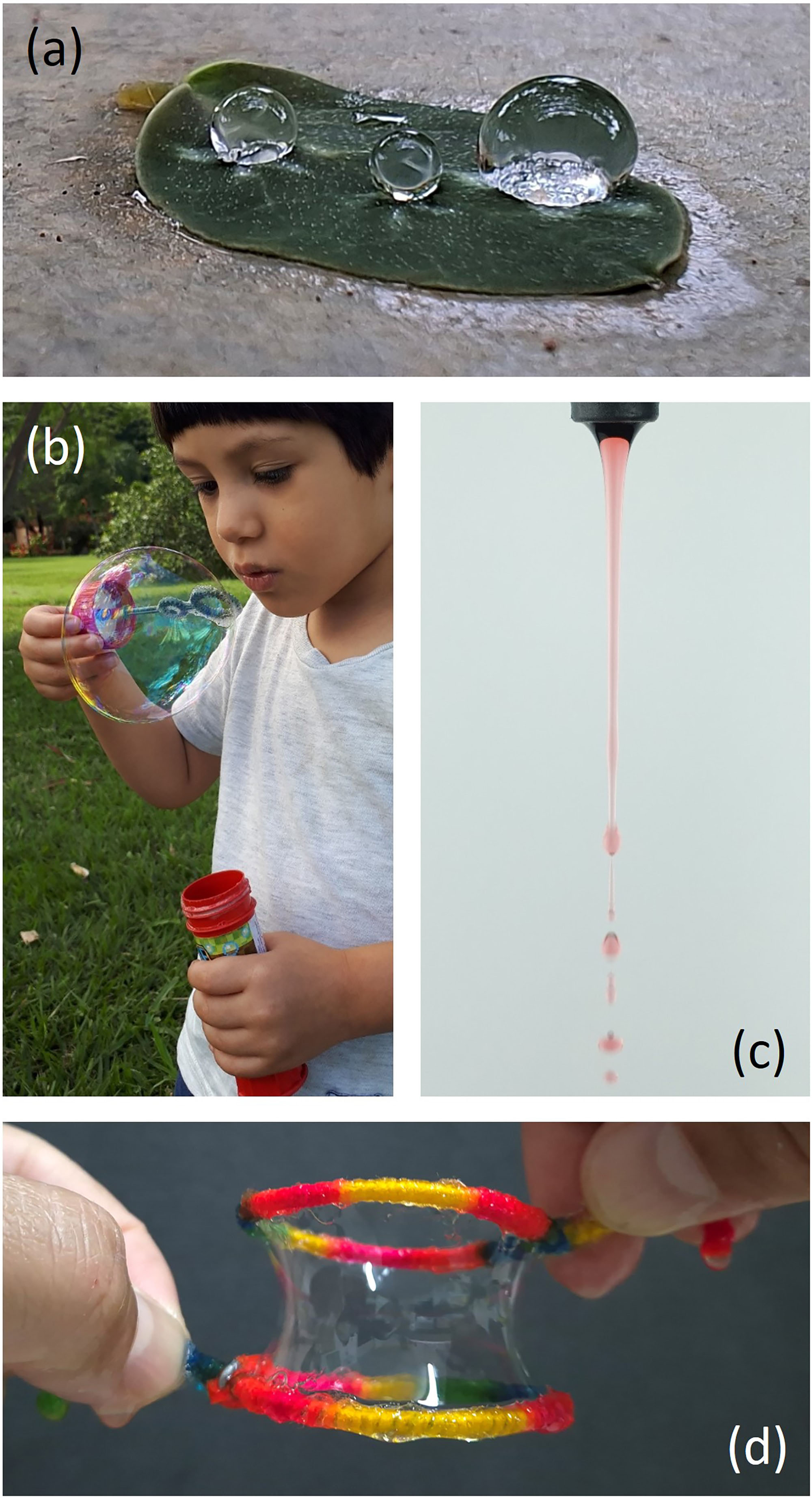
That is, the curvature of any free interface subject to no external forces must be uniform. In this case, condition 38 implies that the surface must be spherical, since among all shapes enclosing the same volume, the sphere has the smallest surface area [¹⁷]. This property explains why spheres are frequently observed in nature, such as in droplets, raindrops and soap bubbles, where surface tension acts to minimize surface area, as seen in Fig. 6.

Figure 6
Everyday examples where surface tension acts to minimize surface area: water droplets (a) and soap bubbles (b) tend to form spherical shapes, while the flow from a faucet (c) presents a cylindrical stream before breaking into drops and a soap film connecting two loops assumes the shape of a catenoid (d).

This phenomenon can also be observed when opening a faucet. It is common to observe the nearly cylindrical stream of water spontaneously breaking into droplets to reduce its surface area (see Fig. 6c) – a phenomenon known as the Plateau-Rayleigh instability [²², ²³].

5.1.1. Soap Films

Consider, for instance, a circular wire loop that has been dipped into and removed from a solution composed of water, soap, and glycerin. Equation 38 indicates that the resulting film on the loop must adopt the shape of a flat disk ($\kappa =0$), since the film surface is open ($\mathrm{\Delta }P=0$). Now consider two such loops that are slowly separated after being dipped and removed from the soap solution. The result is a soap film that smoothly connects the two loops, as seen in Fig. 6d. Due to the symmetry of the setup, the film forms a surface of revolution and, being an open surface ($\mathrm{\Delta }P=0$), it must also be minimal ($\kappa =0$), i.e., a catenoid [²⁴].

A very common method for producing a soap-bubble is to blow air into the film formed on the loop in the previous example, as seen in Fig. 6b. According to Eq. 1, the work required to generate the bubble is given by

(39) $$W=\gamma \mathrm{\Delta }A=\gamma \left(A_b-A_l\right)=2\gamma \left(4\pi R_b^2-\pi R_l^2\right),$$

where $\gamma$ is the surface tension of the solution, and $A_b$, $R_b$, $A_l$ and $R_l$ are the surface areas and radii of the bubble and the loop, respectively. In this expression, the multiplicative factor of 2 accounts for the fact that the soap film consists of a bilayer of soap molecules [²⁵]. For this type of solution, $\gamma \approx 0.003$ N/m [²⁶]. Therefore, under ideal conditions, the work required to form a bubble with $R_b=1$ cm from a loop with $R_l=1$ cm is approximately $W\approx 6$ $\mu$J. The YLE also indicates that the pressure difference between the inside and outside of the bubble should be $\mathrm{\Delta }P=2\gamma /R\approx 60$ $\mu$Pa.

5.1.2. Adhesion

Figure 7 illustrates the contact between two spherical particles of equal radius $b$. If the particles are wet, water will accumulate in the region surrounding the contact point, forming a liquid surface (meniscus) with principal radii of curvature $R_1>0$ and $R_2<0$. In most practical cases, $R_1\gg R_2$, such that we can approximate

(40) $$\frac{1}{R_1}-\frac{1}{R_2}\approx -\frac{1}{R_2}.$$

Figure 7
When two wet spherical particles come into contact, water accumulates in the region around the contact point, forming a liquid surface with curvature. This results in an attractive force between the particles due to the liquid’s surface tension.

In these cases, Eq. 38 indicates that the pressure inside the liquid is $\mathrm{\Delta }P=\gamma /R_2$ lower than the external pressure. This pressure difference acts over a cross-sectional area approximately equal to $\pi R_1^{\text{2}}$, resulting in an attractive force of approximately $\pi \gamma R_1^{\text{2}}/R_2$. From the triangle shown in Fig. 7, we have ${\left(b+R_2\right)}^2=b^2+{\left(R_1+R_2\right)}^2$, which leads to $2b{R}_2=R_1^{\text{2}}+2R_1{R}_2\approx R_1^{\text{2}}$, and thus, the attractive force between the two spheres is

(41) $$F_{att}\approx 2\pi \gamma b.$$

The force depends solely on the particle radius and the liquid’s surface tension. For instance, two wet spheres with radii $b=2.3$ mm are attracted to each other by a force of approximately 1 mN.

5.2. Curvature and gravity

The gravitational field plays a significant role in shaping fluids, especially in systems where surface tension is relatively weak. When gravity is taken into account, the pressure across different points of the interface is no longer uniform; it increases with depth due to the weight of the fluid. This implies that the curvature of the interface may vary with position, thereby affecting the overall shape of the fluid.

Consider the ubiquitous situation of water under the influence of a gravitational field $\overrightarrow{g}=-g\widehat{z}$, with constant atmospheric pressure $P_0$ surrounding it. Since the density of water $\rho$ is much greater than the density of air, the hydrostatic pressure beneath a water column of height $z$ is given by $P=P_0+\rho gz$, which leads to $\mathrm{\Delta }P=\rho gz$. In this case, Eq. 37 becomes

(42) $$\kappa \left(z\right)=\frac{\mathrm{\Delta }P}{2\gamma }=\frac{z}{2{\lambda }^2},$$

where

(43) $$\lambda =\sqrt{\frac{\gamma }{\rho g}}$$

is defined as the capillary length. This characteristic length scale marks the point at which gravitational forces become comparable to surface tension and is frequently used to determine when gravity can be neglected. For water, the capillary length is approximately 2.7 mm. Water bodies in air are dominated by surface tension as long as they are smaller than this length. More generally, this scale sets the upper limit for phenomena such as the maximum size of pendant drops [²⁷], raindrops [²⁸], and water-walking insects [²⁹].

5.2.1. Menisci

Liquids are typically contained in solid vessels with vertical walls. The liquid surface is flat due to gravity, except near the walls, where a meniscus forms. The shape of the meniscus is determined by two factors: the contact angle between the air–water interface and the wall, and the balance between hydrostatic pressure and curvature pressure.

The contact angle arises from the balance between cohesive forces (between molecules of the liquid) and adhesive forces (between the liquid and the solid molecules). It provides a measure of how a liquid spreads upon contact with a solid surface [³⁰]. If the liquid molecules are strongly attracted to the solid molecules, the liquid spreads completely over the solid surface, resulting in a contact angle close to 0°. This is often the case for water on glass, metal, or ceramic surfaces. Generally, if the contact angle with water is less than 90°, the surface is considered hydrophilic; if greater than 90°, the surface is considered hydrophobic.

Figure 8 illustrates the menisci formed along the walls of a tube of radius $a$ and the phenomenon of capillary rise. In tubes with radius much smaller than the capillary length ($a\ll \lambda$), the meniscus inside the tube can be approximated as a spherical cap. The radius of curvature $R$ of this spherical cap equals the tube radius $a$ when the contact angle ${\theta }_c$ is zero, and more generally, it is $a/\cos {\theta }_c$. This spherical cap is concave in air and convex in water, meaning the pressure inside the water column is lower than atmospheric pressure, since it is this pressure difference that drives the liquid upward. According to Eq. 20, the curvature of this spherical interface is $\kappa =-1/R=-\cos {\theta }_c/a$ and $\mathrm{\Delta }P=-\rho gH$. Note that the adhesive force between liquid molecules and the tube walls defines the curvature of the interface, which in turn generates a pressure difference as a water pump. The height $H$ of the capillary rise can be obtained from Eq. 42:

(44) $$\frac{\cos {\theta }_c}{a}=\frac{H}{2{\lambda }^2},$$

Figure 8
The menisci formed along the walls of a tube of radius $a$ and the phenomenon of capillary rise. If $a\ll \lambda$, the meniscus inside the tube can be approximated as a spherical cap with radius $R=a/\cos {\theta }_c$. The meniscus on the outside of the tube takes the shape of a surface of revolution generated by the planar curve $z\left(x\right)$.

from which we derive Jurin’s Law [³¹]:

(45) $$H=\frac{2{\lambda }^2\cos {\theta }_c}{a}.$$

In a glass capillary tube with radius $a=1$ mm in contact with water, ${\theta }_c\approx$ 15^∘[³²] and the predicted height is $H\approx$ 13.5 mm.

The meniscus on the outside of the tube takes the shape of a surface of revolution generated by the planar curve $z\left(x\right)$, as illustrated in the Fig. 8. Substituting Eq. 14 into Eq. 42 yields the general equation describing the shape of the meniscus:

(46) $$\frac{z^{\prime \prime }}{{\left(1+z^{\prime 2}\right)}^{3/2}}+\frac{z^{\prime }}{x{\left(1+z^{\prime 2}\right)}^{1/2}}=\frac{z}{{\lambda }^2}.$$

Different methods can be employed to solve this nonlinear differential equation [³³]; however, it is particularly insightful to examine certain limiting cases. One such case occurs when $a\ll \lambda$. More specifically, in the situation where ${\theta }_c=0^{\circ }$ (e.g., when the tube is highly hydrophilic) and near the contact line ($x<\lambda$) it can be considered that $\mathrm{\Delta }P\approx 0$, i.e., water molecules are adhered to the wall of the tube and, therefore, the hydrostatic pressure is zero, to the extent that gravity can be completely neglected in Eq. 42. In other words, in the vicinity of the tube, the mean curvature is effectively zero, and therefore, the planar curve corresponds to a catenary, while the meniscus surface forms a catenoid. The solution 23 for the case ${\theta }_c=0^{\circ }$, defined by the boundary condition $z^{\prime }=\infty$ at $x=a$, is given by

(47) $$z\left(x\right)=h-a\mathrm{}{\cosh }^{-1}\left(\frac{x}{a}\right),$$

where $h$ is the height of the meniscus on the outside. This height can be estimated [³⁴] by truncating the profile with the condition $z\left(\lambda \right)=0$, which yields

(48) $$h=a\mathrm{}{\cosh }^{-1}\left(\frac{\lambda }{a}\right)\approx a\ln \left(\frac{2\lambda }{a}\right).$$

A more general and accurate calculation [³⁵] provides that, for ${\theta }_c<{90}^{\circ }$,

(49) $$h\approx \left(a\mathrm{}\cos {\theta }_c\right)\ln \left(\frac{4\lambda }{a\left(1+\sin {\theta }_c\right)}-0.577\right).$$

Another interesting case is the meniscus with a small inclination, defined by the limit $z^{\prime }\ll 1$, which is always valid far from the tube. In this limit, Eq. 46 becomes

(50) $$z^{\prime \prime }=\frac{z}{{\lambda }^2},$$

a linear equation that can be solved easily. Applying the boundary conditions $z\left(\infty \right)=0$ and $z^{\prime }\left(a\right)=-\cot {\theta }_c$, the solution to Eq. 50 is

(51) $$z\left(x\right)=\left(\lambda \cot {\theta }_c\right)e^{-\left(x-a\right)/\lambda },$$

indicating that the meniscus height decays exponentially with rate constant $\lambda$.

5.2.2. Volume of a Pendant Drop

Figure 9 illustrates a pendant drop of water of volume $V$ hanging from the orifice of a faucet with radius $r$. This drop detaches and falls when its weight $F_g=-mg$ exceeds the force holding it in place. According to Eq. 25, this force is $F_{\gamma }=2\pi \gamma r$, and therefore, the critical condition for detachment is $mg=\rho Vg=2\pi \gamma r$. In other words, the drop detaches when it reaches the volume

(52) $$V=2\pi r{\lambda }^2.$$

Figure 9
A pendant drop forming at the opening of a faucet with radius $r$. The drop remains attached until its weight $F_g$ exceeds the force holding it in place due to surface tension $F_{\gamma }$.

Note that Eq. 52 can be rewritten in dimensionless form as

(53) $$B_{o}v=2\pi ,$$

where $v=V/r^3$, and

(54) $$B_o={\left(\frac{r}{\lambda }\right)}^2=\frac{\rho g{r}^2}{\gamma }$$

is the Bond number. This dimensionless number quantifies the relative importance of gravity-induced forces compared to surface tension. Gravity can be considered the dominant force when $B_o\gg 1$, whereas surface tension dominates when $B_o\ll 1$. If $B_o\approx 1$, both gravity and surface tension contribute comparably. For a typical garden faucet, with $r=5$ mm, we find $B_o=3.4$. In the case of a syringe orifice with $r=0.5$ mm, we obtain $B_o\approx 0.035$.

5.2.3. Puddle Height

Consider a liquid droplet deposited on a flat, horizontal solid surface. If the droplet is small, with a radius $r$ smaller than $\lambda$, such that $B_o\ll 1$, surface tension dominates. This causes the curvature of the interface to be constant, and thus the droplet adopts the shape of a spherical cap whose edges intersect the substrate at a contact angle ${\theta }_c$ (see Fig. 10a). If the droplet is large and heavy (i.e., a puddle), such that $B_o\gg 1$, it is flattened by gravity. At equilibrium, it takes the shape of a flattened liquid “pancake” of thickness $D$ (see Fig. 10b). This thickness can be determined as follows.

Figure 10
Formation of a water puddle on a flat, horizontal solid surface. For small droplets (a), the surface adopts the shape of a spherical cap, while for large drops or puddles (b), gravity dominates, flattening the liquid. The maximum depth of a puddle on a flat surface can be calculated by considering the curvature of the liquid interface (c).

Figure 10c shows the lateral profile of a resting water puddle on a flat, horizontal solid surface. The origin of the coordinate system is placed at the point where the profile begins to descend. It is wide, with a front edge extending along a straight line perpendicular to the page. In this case, the edge profile curves only in the vertical plane, so one of the two principal radii of curvature is infinite. Therefore, Eq. 42 reduces to

(55) $$\frac{1}{R}=\frac{z}{{\lambda }^2},$$

where $R$ is the principal radius of curvature at a point on the surface located at height $D-z$. Consider an infinitesimal arc length $dl$, extending from $z$ to $z+dz$, subtending an infinitesimal angle $d\theta$ with radius $R$. According to Fig. 10c, we have $dl=Rd\theta$ and $dz=dl\sin \theta$. These two expressions, together with Eq. 55, yield

(56) $$zdz={\lambda }^2\sin \theta d\theta .$$

Integrating both sides, we obtain

(57) $${\int }_0^{D}z\mathit{d}z={\lambda }^2{\int }_0^{{\theta }_c}\sin \theta d\theta$$

and thus,

(58) $$D=\lambda \sqrt{2\left(1-\cos {\theta }_c\right)}.$$

According to Eq. 58, the maximum depth of a water puddle on a flat, horizontal glass surface (${\theta }_c\approx {15}^{\circ }$) is $D\approx 0.7$ mm. If the surface is made of Teflon (${\theta }_c\approx {120}^{\circ }$), the puddle depth increases to $D\approx 4.7$ mm.

6. Final Remarks

The Young-Laplace Equation provides a remarkable relationship between the pressure difference across an interface, its curvature, and its surface tension. It is a fundamental result in physics and engineering, with practical applications across a wide range of fields. In this work, we discussed the physical origins and consequences of surface tension, as well as the mathematical concept of curvature. The YLE was derived from the principle of mechanical equilibrium using two equivalent, yet conceptually complementary, approaches. Finally, several examples were presented to illustrate how the YLE can be used to explain a variety of intriguing everyday phenomena. This text is intended to be both comprehensive and accessible to readers with a basic understanding of calculus and classical mechanics, making it a useful resource for teaching, research, and science communication.

Acknowledgments

The authors would like to thank Pedro Augusto Matos Rodrigues, Fábio Ferreira Monteiro and Luiz Antonio Ribeiro Junior for their insightful comments that contributed to this work.

Data Availability

The entire dataset supporting the results of this study is published in the article.

References

• ^[1] T. Young, Philosophical Transactions of the Royal Society of London 95, 65 (1805).
• ^[2] P.S. Laplace, Traité de Mécanique Céleste (Courcier, Paris 1805), v. 4.
• ^[3] F. Hawksbee, Physico-mechanical Experiments on Various Subjects (R. Brugis, London, 1709).
• ^[4] J.A. Segner, Comment. Soc. Reg. Gotting 1, 301 (1751).
• ^[5] Y. Pomeau, in: 5th Warsaw School of Statistical Physics (Warsaw, 2013).
• ^[6] H. Lamb, Statics: including hydrostatics and the elements of the theory of elasticity (Cambridge University Press, Cambridge, 1946), 3 ed.
• ^[7] L. Landau and E. Lifshitz, Fluid Mechanics (Pergamon Press, Oxford, 1987), 2 ed.
• ^[8] R. Defay and I. Prigogine, Surface Tension and Adsorption (Longmans, Green & Co., London, 1966).
• ^[9] A.W. Adamson and A.P. Gast, Physical Chemistry of Surfaces (Wiley, New York, 1997), 6 ed.
• ^[10] P.G. de Gennes, F. Brochard-Wyart and D. Quéré, Capillarity and Wetting Phenomena (Springer, Paris, 2003).
• ^[11] H.J. Butt, K. Graf and M. Kappl, Physics and Chemistry of Interfaces (Wiley-VCH Verlag GmbH & Co., Weinheim, 2003).
• ^[12] F. Mugele and J. Heikenfeld, Electrowetting: Fundamental Principles and Practical Applications (Wiley, Weinheim, 2019).
• ^[13] J. Pellicer, V. García-Morales and M.J. Hernández, Phys. Educ. 35, 126 (2000).
• ^[14] L.M. Siqveland and S.M. Skjæveland, Capillarity 4, 23 (2021).
• ^[15] F. Behroozi, Phys. Teach. 60, 358 (2022).
• ^[16] J.N. Israelachvili, Intermolecular and Surface Forces (Academic Press, London, 2011), 3 ed.
• ^[17] R. Osserman, Bull. Amer. Math. Soc. 84, 1182 (1978).
• ^[18] M.P. Carmo, Differential Geometry of Curves and Surfaces (Dover, New York, 2016), 2 ed.
• ^[19] R. Goldman, Computer Aided Geometric Design 22, 632 (2005).
• ^[20] J.B. Gil, Boletín de la Asociación Matemática Venezolana XII, 251 (2005).
• ^[21] F. Behroozi, European Journal of Physics 35, 055007 (2014).
• ^[22] J. Plateau, Experimental and Theoretical Equilibrium State of Liquids Subjected to Molecular Forces Only (Trübner and Co., London, 1873), 3 ed.
• ^[23] L. Rayleigh, Proc. London Math. Soc. 10, 4 (1878).
• ^[24] M. Ito and T. Sato, European Journal of Physics 31, 357 (2010).
• ^[25] C. Isenberg, The Science of Soap Films and Soap Bubbles (Tieto, Clevedon, 1978).
• ^[26] A. Sane, S. Mandre and I. Kim, J. Fluid Mech. 841, 841 (2018).
• ^[27] O.E. Yildirim, Q. Xu and O.A. Basarana, Phys. Fluids 17, 062107 (2005).
• ^[28] K. Loftus and R.D. Wordsworth, Journal of Geophysical Research: Planets 126, e2020JE006653 (2021).
• ^[29] D.L. Hu, B. Chan and J.W.M. Bush, Nature 663, e2020JE006653 (2003).
• ^[30] P.G. de Gennes, Rev. Mod. Phys. 57, 827 (1985).
• ^[31] J. Jurin, Phil. Trans. R. Soc. 30, 739 (1718).
• ^[32] V.P. Carey, Liquid-Vapor Phase-Change Phenomena: An Introduction to the Thermophysics of Vaporization and Condensation Processes in Heat Transfer Equipment (CRC Press, Boca Raton, 2020), 3 ed.
• ^[33] Y. Tang and S. Cheng, Journal of Colloid and Interface Science 533, 401 (2019).
• ^[34] D. Quéré and J.M. Di Meglio, Advances in Colloid and Interface Science 48, 141 (1994).
• ^[35] D.F. James, J. Fluid Mech. 63, 657 (1974).

Edited by

• Editor-in-Chief:
  Marcello Ferreira https://orcid.org/0000-0003-4945-3169

Publication Dates

• Publication in this collection
  16 Mar 2026
• Date of issue
  2026

History

• Received
  21 Sept 2025
• Reviewed
  27 Jan 2026
• Accepted
  28 Jan 2026