A short driven Foucault pendulum at 26.9° S latitude

Abstract

In this paper it is discussed the construction of a short Foucault pendulum (2.4 meters long, compared to the several dozen meters typically found in museums and science centers). The pendulum is driven by a standard electromagnet and suspended using a small pin vise. A magnetic sensor is placed directly beneath the pendulum’s equilibrium point to track its motion, enabled by a small neodymium magnet attached to the bottom of the bob. The sensor is connected to an Arduino UNO board (ATmega328P), which processes the readings to control the electromagnet that provides controlled impulses to the pendulum, while also tracking the precession angle of the pendulum’s oscillation plane. This method eliminates the need for a secondary detection coil, commonly employed in similar setups, thereby simplifying the electronic circuit compared with other implementations. Using this approach, it was found a precession rate of 6.8 $\pm$ 0.3 °/h, in agreement with the expected theoretical prediction for our latitude.

Keywords:
Foucault pendulum; Coriolis effect; Airy precession

1. Introduction

A small number of classical physics experiments stand out for the remarkable ingenuity of their underlying principles, almost like Columbus’ egg, so that once they are explained or demonstrated, their logic becomes immediately clear. Notable examples include Eratosthenes’ measurement of the Earth’s radius, the legendary account of Galileo supposedly dropping spheres from the Tower of Pisa, and Thomas Young’s renowned double-slit experiment with light. In the same spirit, Foucault’s pendulum, introduced by Léon Foucault in 1851, provides an elegant demonstration of the Coriolis effect in a rotating reference frame [¹].

Although these experiments may seem simple to set up, there are important subtleties that must be addressed to perform them successfully. In the case of Foucault’s pendulum, several challenges must be overcome to obtain the expected results. This is because the effect to be observed is the precession of the pendulum’s plane of oscillation, and this effect is very subtle over a short period. For a given latitude $\lambda$ and sidereal period $T_s$, the expected period for a complete turn of the plane of oscillation is given by [²]

(1) $$T=\frac{T_s}{\sin \lambda },$$

and the precession rate, $\text{Ω}$, is

(2) $$\text{Ω}=\frac{{360}^{\circ }}{T}=360\frac{\sin \lambda }{T_s}.$$

Thus, for a sidereal time of $T_s=$ 23 hours, 56 minutes and 4.0905 seconds (or 23.9344696 h) [³], a pendulum located exactly at the South Pole would have its plane of oscillation precessing at approximately 15.041^∘/h, while at our location (Blumenau, SC, Brazil, latitude 26.9208^∘ S) the expected precession is 6.810^∘/h, both counterclockwise as seen from above.

To clearly observe such an effect, the pendulum must maintain its motion for several hours. However, oscillations are damped by air resistance. A common solution to this problem is to attach a small magnet to the bottom of the pendulum’s bob and use a coil to generate a magnetic field that either pushes or pulls the bob. When properly calibrated, the coil provides just enough energy to maintain the desired amplitude.

In this paper it is described the construction of a short Foucault pendulum (2.4 meters long, as opposed to the several-dozen-meter pendulums typically found in museums and science centers) driven by a standard electromagnet and suspended from a small pin vise. A magnetic sensor is positioned just below the pendulum’s equilibrium position to track its motion via the attached magnet. The sensor is connected to an Arduino UNO board (ATmega328P), which uses the readings to control the electromagnet and monitor the angle of the oscillation plane. Additionally, a Charron ring is placed beneath the suspension point to reduce the elliptical motion that naturally arises.

Small-length Foucault pendulums are not a novelty; several studies have discussed the challenges of maintaining steady motion without introducing anisotropies into the system. For example, the work of Crane describes the construction of a 70 cm Foucault pendulum “wall clock” [⁴] (and even a 15 cm version is mentioned), reporting a precession rate of $10.2\pm 0.2$^∘/h at a latitude of 42.28^∘ N, where the expected value is 10.12 ^∘/h. Plewes also reports a small 65.4 cm pendulum [⁵], driven by a coil that interacts with a permanent magnet attached to the bob, while measurements are performed using a magnetic sensor and an Arduino. In that case, a precession rate of 10.31 ^∘/h was obtained, which is within 0.54% of the expected value for a latitude of 43.718^∘ N. In both studies, a sensor coil is used to detect the approach or departure of the bob and to trigger the circuit responsible for the drive mechanism. In contrast, the present work does not rely on a sensor coil; instead, the same magnetic sensor is used both to determine the azimuth of the oscillation plane and to detect the passage of the bob through the center, allowing a microcontroller to control the triggering mechanism of the driving electromagnet.

The following section details each of the components mentioned above. Section 3 discusses the magnetic forces and elliptical movement, Section 4 presents the data obtained and Section 5 provides an analysis of the results. Section 6 concludes with some remarks.

2. Mechanics and Electronics

The system can be divided into two main parts: mechanical and electronic. The mechanical part includes the suspension system that supports the pendulum, the Charron ring, the cable, and the bob with the attached magnet. The electronic part consists of the electromagnet, the magnetic sensor, the Arduino board, an H-bridge, and a power supply. Each component and its respective function are described below.

2.1. Suspension system

One of the main limitations in constructing a Foucault pendulum is its length. Some of the most famous examples include the pendulum at the Panthéon in Paris, which is 67 meters long and has a bob weighing approximately 28 kg, and the 26-meter-long pendulum at the Franklin Institute in Philadelphia, featuring an impressively heavy bob of 816 kg [⁶]. Longer pendulums will keep its movement for a greater time without a driving mechanism and are less susceptible to intrinsic precession (as discussed in Section 2.2).

On the other hand, our lab is only 3 meters high, and it is not possible to suspend the pendulum from the ceiling (Figure 1). Following Crane’s approach [⁴], the pendulum was suspended on a steel rack support fixed to the wall, as shown in Figure 2. The support is made of a $150\mathrm{mm}\times 150$ mm steel square plate with a thickness of 5.0 mm. It has a central hole with an $\mathrm{M8}\times 0.75$ mm thread, where the pin vise that holds the cable is fixed. Also, on this plate, a pulley was welded so that the cable could enter vertically on the pin vise. The cable is anchored to the upper steel plate to prevent damage in case it escapes.

Figure 1
On the right: image of the complete setup. On the left: vertical dimensions, with an uncertainty of $\pm$ 0.1 cm. The cable seen above is from the webcam used to monitor the system.

Figure 2
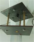
Photograph of the suspension system. The pin vise, in the middle of the upper plate, is a small quick change keyless drill chuck for rotary tools with a length of 2.5 cm. On the lower plate, the cable is touching the Charron ring adapter (yellow).

This plate also has six 8 mm holes, three of them used to attach the plate to the support and the other three to hold three brass cylinders. Those act as spacers to another square steel plate, the Charron ring, with a 10 mm hole in its center, aligned with the cable. This arrangement, presented in [⁷], simplifies alignment of the system. The details of the support are shown in Figure 3 and Table 1.

Figure 3
Schematic drawing of the suspension system.

Table 1
Components of the suspension system.

No.	Component
1	Pulley
2	Pin vise adapter
3	M6 bolt to attach the brass spacer
4	Spring washer
5	Brass spacer (100.00 mm long, $\varphi =9.00$ mm, M6 thread)
6	6 mm hole to attach to the wall support
7	Bolt to anchor the cable
8,9	150 mm $\times$ 150 mm square steel plate, 5.0 mm thick
10	Charron ring with 10 mm central hole

It is worth mentioning that, also inspired by [⁷] (which employs a wire die to hold the cable), it was tested an alternative method of securing the cable instead of using the pin vise. An extruder bolt (commonly used in 3D printers) was employed, featuring a 0.7 mm hole, the exact diameter of the cable. However, this setup did not provide a sufficiently stable fixed point for the pendulum, and any deviation from a perfectly circular hole caused the oscillation plane to become constrained to a fixed direction.

2.2. Charron ring and elliptical motion

It was demonstrated by G. B. Airy that the trajectory of an ideal spherical pendulum, when projected on the horizontal plane, describes a small elliptical movement. Since the period of the pendulum to go back and forth is different from the time it takes to go around the elliptical path, a precession occurs. This intrinsic precession, in the long run, could overcome the precession due to the Coriolis force or even cancel it, keeping the pendulum oscillating in the same fixed plane [⁸]. This precession is related to the ellipse parameters in the following form:

(3) $${\text{Ω}}_{\text{prec}}=\frac{3A}{4l^{2}T},$$

where $A$ is the area enclosed by the ellipse, $l$ is the pendulum length, and $T$ is its period. Therefore, larger pendulums will present a smaller intrinsic precession.

To deal with this intrinsic precession, a Charron ring is used in order to reduce the elliptical motion that the pendulum undergoes, even when the initial release is intended to be purely radial. In practice, any axial asymmetry of the system could introduce a small tangential component, which results in an undesired elliptical trajectory [⁹].

When the suspension cable comes into contact with the ring, the resulting friction selectively attenuates the tangential component of the motion, thereby favoring oscillations confined to a vertical plane. This effect stabilizes the trajectory and ensures more accurate observation of the precession associated with the Earth’s rotation [¹⁰].

The efficiency of the Charron ring depends on both its positioning and its diameter, which are typically chosen according to the suspension height and the desired oscillation amplitude. If the ring is placed too close to the bob, the damping may be excessive, leading to significant energy loss and a shortened observation time. Conversely, if it is placed too high, the reduction of ellipticity becomes ineffective. An optimal configuration therefore balances damping of the tangential motion with preservation of the oscillation period (about a tenth of the way down from the top) [¹¹]. The diameter is directly related to the amplitude as well and must be such that the cable barely touches the ring at its maximum amplitude.

Historically, the Charron ring was introduced in the 20th century as an improvement for public demonstrations of the Foucault pendulum, where long-term stability and visual clarity were essential. Although there are alternative systems such as eddy-current damping proposed in modern implementations [¹²], the Charron ring remains one of the simplest and most robust methods for minimizing unwanted elliptical oscillations.

The bolts numbered 3 in Table 1 can be adjusted to level the Charron ring. Since the plates were drilled together, the central hole where the pin vise is fixed is concentric with the hole in the Charron ring (and the same applies to the brass spacers). Thus, although lateral adjustment of the lower plate is not possible, the design ensures it is centered relative to the upper plate.

For an amplitude $\theta ={2.5}^{\circ }$, the Charron ring has a diameter of 7 mm. A 3D-printed adapter (shown in yellow in Figure 2) is used to adjust the diameter for other amplitudes. An analysis of the elliptical motion is made in Section 4.1 and its implications are discussed in Section 5.3.

Although the Charron ring quickly damps any residual elliptical component, the long-term stability of the plane of oscillation depends primarily on the isotropy of the entire system (suspension, driving mechanism, and mass distribution), as will be discussed in Sections 4 and 5.

2.3. Oscillating mass

The suspension system consists of a steel, nylon-coated fishing cable with a diameter of 0.70 mm. This cable is attached to an iron ball (an Olympic throwing ball with a mass of 7 kg and a 12 cm diameter) by means of an M10 bolt, which has a 0.70 mm hole drilled through its center and is pressed into the bottom of the threaded hole. On the opposite side of the ball, a small neodymium magnet was embedded in an undercut at the bottom, as shown in Figures 4(a) and 4(b). The pendulum has a total length of 2.4 meters. It can be seen that the ball is not perfectly round and has some irregularities that, in principle, could jeopardize the symmetry of the system. A discussion about the drag force and its influence upon the precession rate is given in Section 5.

Figure 4
(a) Top of the bob, showing an M10 bolt with a 0.70 mm hole. (b) Bottom of the bob, with a 25 mm diameter neodymium magnet.

2.4. Electromagnet and magnetic sensor

In order to sense the passage of the pendulum through its equilibrium point, a QMC5883L magnetic sensor is used. It is powered by 5 V and can detect the magnetic fields in the range of $\pm 8$ G with a resolution of 0.1 mG in the $x$, $y$, and $z$ directions. The sensor is connected to an Arduino board (through an RJ11 connector) that reads the signal and processes it. This sensor was enclosed in a 3D-printed case and attached to a linear $xy$ stage that allowed its centering with the rest of the system (Figure 5, items 4–7). It is worth to note that a stronger electromagnet will be needed for greater amplitudes or a heavier bob, so its magnetic field may not be in the range of the sensor and the system may not work properly.

Figure 5
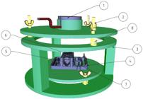
Schematic drawing of the 3D-printed support for the electromagnet and magnetic sensor. PETG filament was used, with 30% infill for every piece.

To compensate for the energy losses caused by air drag, a standard approach is to position a coil beneath the equilibrium point of the pendulum so that it can either push or pull the bob. In the present setup, an electromagnet was driven by an Arduino board through a BTS7960 H-bridge, which enables switching the polarity of the current in the coil. This configuration allows the pendulum bob, equipped with a small permanent magnet, to be periodically accelerated or decelerated. With the H-bridge powered by a 24 V, 1 A supply, the voltage applied to the electromagnet can be regulated, thereby providing precise control over the energy delivered to the system. This specific H-bridge is capable of providing a continuous current of up to 43 A and tension from 5.5 V to 27 V, so it must match the electromagnet specification.

Usually, in setups like this one that use a coil to deliver energy to the pendulum, a second coil is used as a sensor. In this context, this sensor coil is responsible for indicating whether the pendulum is approaching the center or moving away. This is extremely important, since the instants when the electromagnet is turned on and off are crucial to maintain the desired amplitude. This movement was tracked using the $z$-axis measurements of the magnetic sensor, eliminating the necessity of a second coil and keeping the electronic circuit simpler than usual implementations of this kind. The advantage of this method is a simpler electronic circuit, eliminating several componentes. Moreover, the implementation of a software controlled driving system allows for the remote control of the trigger parameters if desirable.

2.5. Electronic circuit and data acquisition

The electronic part is responsible for reading the values from the magnetic sensor and controlling the electromagnet. It is also used to determine the angular variation of the pendulum’s plane of oscillation. The schematic of the electronic circuit is depicted in Figure 6.

Figure 6
Schematic circuit for the control system.

The $z$ component of the magnetic field, $B_z$, can be used to calculate the period of the pendulum. The algorithm uses this period to determine when the electromagnet should be on or off, pushing or pulling. After several tests, it was found that the optimal configuration is such that the electromagnet turns on to pull the bob at a time $t_e=200$ ms after it reaches the turning point, for a duration $t_p=100$ ms. This configuration maintains an amplitude $\theta ={2.5}^{\circ }$, so that the cable just touches the Charron ring.

The $x$ and $y$ components of the magnetic field were used to determine the angle of the plane of oscillation with respect to an arbitrary direction. A trigger was set to collect the $x$ and $y$ data every time $t_m=600$ ms after the pendulum passed through the center. Each pair of measurements was used to determine the direction of the plane of oscillation. A Python script acquires the data via the serial port and displays in real time the precession rate of the plane of oscillation, the measured angle, and a moving average of the last 20 measurements. The data is sampled every 30 ms and the uncertainty in time is $\pm$2 ms.

The system containing the sensor and the electromagnet is enclosed in a 3D-printed platform that allows for adjustments in the orientation of both components. All parts of this assembly are made of plastic to avoid undesired magnetic interactions. The sensor and electromagnet cables are 2 meters long and are twisted together to minimize electromagnetic interference. This setup can be seen in Figure 7.

Figure 7
Photograph of the lower part of the system. The vertical distance between the bob (at rest) and the electromagnet is 30 mm.

The script running on the Arduino performs the following tasks during half oscillation, as shown in Figure 8:

Figure 8
Timeline of the control system during a half period, $T/2$.

1. Reads data from the magnetic sensor;

2. Monitors the $z$-axis component to determine the oscillation period (this value reaches a maximum when the pendulum passes through the equilibrium position);

3. At a time $t_m$ milliseconds after the pendulum passes through the center, the $x$ and $y$ components of the magnetic field, $B_x$ and $B_y$ respectively, are sampled. This is done twice during each oscillation;

4. Calculates the orientation angle of the oscillation plane using the measurements above;

5. Activates the electromagnet $t_e$ milliseconds after the pendulum reaches the maximum amplitude, keeping it on for $t_p$ milliseconds to pull the bob;

6. Sends the data to a computer, where a Python script displays, in real time, a graph of the oscillation plane angle vs. time.

A webcam was placed directly above the pendulum to enable remote adjustment of the parameters and to record its motion. Once the parameters are adjusted and the pendulum is set in motion, it will continue oscillating indefinitely without further adjustments.

2.6. Alignment of the system

It is crucial that the system remains aligned with the equilibrium position. To this end, the following procedure was adopted after suspending the bob using the steel cable and locking it in the pin vise: a bubble level with a precision of $\pm {0.1}^{\circ }$ is used to verify that the upper plate is parallel to the ground, and corrections can be made by adjusting the screws, such as screw No. 6 in Figure 3, acting on the spring washers.

Next, fine adjustments are made to the other plate (the Charron ring) to center both the ring and the cable. The ideal configuration is such that the cable lightly contacts the ring during each swing and remains in contact for the same amount of time in each direction. This is verified visually by observing whether the cable, after ceasing contact on one side, maintains symmetrical contact with the diametrically opposite side. Small corrections ensure that the ring remains centered with respect to the cable.

The next step is to align the electromagnet with the bob, which is also performed visually. For this purpose, a pointer tool with a magnet at its base was designed; it attaches to the center of the bob, leaving a 0.7 mm tip to be aligned with a target placed directly above the electromagnet, ensuring a precision of 0.5 mm.

Finally, the magnetic sensor is aligned with the system. The sensor is positioned so that the reading on the $z$-axis is maximized, ensuring that it is precisely aligned beneath the magnet. In Figure 9 can be seen that the variation of the magnetic field in the $z$ direction, $B_z$, as the pendulum oscillates back and forth. The period can be determined from the peaks of the graph, yielding a result of $T=3.108\pm 0.003$ seconds.

Figure 9
(a) System misalignment. (b) System aligned. The frequency of the senoidal fit is $\omega =4.043\pm 0.004$ rad/s.

It is interesting to note that the valleys alternate in depth in Figure 9(a), meaning that the pendulum reaches farther on one side than on the other. Since the magnetic sensor is aligned with the pendulum at equilibrium and maximizes the $B_z$ field reading, it is possible to infer that this variation in valley depths is due to a misalignment of the Charron ring. On the other hand, Figure 9(b) shows a more symmetrical pattern, with better alignment.

3. Magnetic Interaction and Forces

To observe the precession of the plane of oscillation due to the Coriolis force, it is important that the driving magnetic force does not introduce any transverse component to the pendulum (i.e., any non-radial force on the $xy$ plane). If the electromagnet is perfectly aligned with the center of the system, no transverse force is expected. It is instructive to see how this interaction would be in a first approximation, considering the dipole approximation, to understand that the direction of the magnetic force is essentially radial (on the $xy$ plane) and vertical ($z$ axis). Supposing the magnetic moment of the electromagnet as ${\mathbf{m}}_1$ and that of the permanent magnet as ${\mathbf{m}}_2$, and $\mathbf{r}=r\widehat{\mathbf{r}}$ the distance vector between them, the force would be [¹³]

(4) $$\mathbf{F}=\frac{3{\mu }_0}{4\pi r^4}[({\mathbf{m}}_1\cdot \widehat{\mathbf{r}}){\mathbf{m}}_2+({\mathbf{m}}_2\cdot \widehat{\mathbf{r}}){\mathbf{m}}_1+({\mathbf{m}}_1\cdot {\mathbf{m}}_2)\widehat{\mathbf{r}}-5({\mathbf{m}}_1\cdot \widehat{\mathbf{r}})({\mathbf{m}}_2\cdot \widehat{\mathbf{r}})\widehat{\mathbf{r}}],$$

with no transverse component on the $xy$ plane.

However, if a displacement $\delta$ of the electromagnet in the $xy$ plane is considered, a transverse component of the magnetic force is introduced, as shown in Figure 10. Let us make the assumption that the force is on the $xy-$ plane, with $F_{M\widehat{r}}=4.6\times {10}^{-3}$ N (see Appendix A), so that the transverse component would be $F_{M⟂}=ϵF_{M\widehat{r}}\approx \frac{\delta }{r}{F}_{M\widehat{r}}$. For $r=0.1$ m and assuming a displacement $\delta =1.0\times {10}^{-3}$ m, it is found $F_{M⟂}=4.6\times {10}^{-5}$ N. Considering that the electromagnet acts for just a time interval $t_p=100$ ms, the magnetic impulse in the transverse direction is given by $J_M=F_{M⟂}{t}_p=\left(4.6\times {10}^{-5}\text{N}\right)\cdot \left(0.1\text{s}\right)=4.6\times {10}^{-6}\text{N}\cdot \text{s}.$

Figure 10
Diagram depicting the magnetic radial force ${\mathbf{F}}_{M\widehat{r}}$ due to the interaction of the permanent magnet and electromagnet separated by a distance $r$. If the electromagnet is off center by a distance $\delta$, a transverse force, ${\mathbf{F}}_{M⟂}$ (in red), appears and can interfere with the pendulum precession.

On the other hand, the Coriolis force is given by [¹⁴]

(5) $$F_C=2m\text{Ω}\sin \lambda v,$$

where $m$ is the mass of the bob, $\text{Ω}$ is the Earth’s rotation angular speed, $\lambda$ is the latitude and $v$ the speed of the bob. Considering $\text{Ω}=7.292\times {10}^{-5}$ rad/s, $\lambda =-{26.9}^{\circ }$, $m=7$ kg, and $v=v_{\max }=0.20$ m/s (for an amplitude of 2.5^∘), it was found $F_C=9.2\times {10}^{-5}$ N. If the velocity of the bob is given by $v\left(t\right)=v_{\max }\sin \frac{2\pi }{T}t$, the impulse due to the Coriolis force is given by $J_C=\int F_C\mathit{d}t$:

(6) $$\begin{array}{l}{J}_C={\int }_0^{T/2}2m\text{Ω}\sin \lambda v_{\max }\sin \left(\frac{2\pi }{T}t\right)\mathit{d}t\\ =2m\text{Ω}\sin \lambda v_{\max }{\int }_0^{T/2}\sin \left(\frac{2\pi }{T}t\right)\mathit{d}t\\ =2m\text{Ω}\sin \lambda v_{\max }\frac{T}{\pi }\\ =\left(9.2\times {10}^{-5}\text{N}\right)\frac{\left(3.1\text{s}\right)}{\pi }=9.1\times {10}^{-5}\text{N}\cdot \text{s}.\end{array}$$

Comparing the two results, it can be seen that $\frac{J_M}{J_C}\approx 0.05$, that is, the impulse of the transverse magnetic force is a twenty times smaller than the Coriolis force impulse, if the electromagnet is 1 mm off center. Since the centering precision is about 0.5 mm, the transverse magnetic impulse would be very small. Similar argument is valid if the electromagnet is perfectly centered but the bob describes an elliptical motion. The possible influence of this transverse impulse is discussed in Section 5.

4. Results

4.1. Angle measurement and elliptical motion

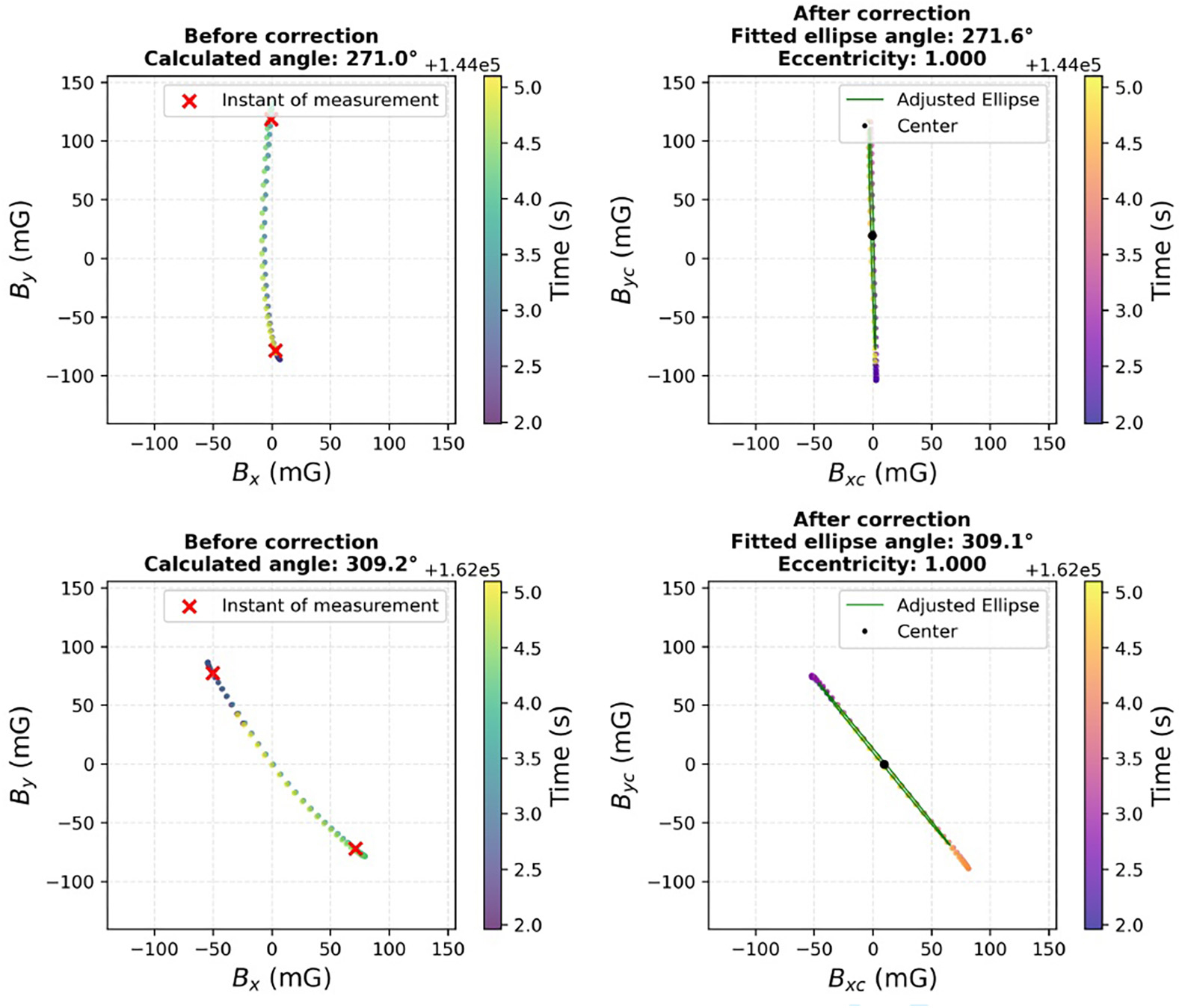
The zero-angle direction is defined by the orientation of the magnetic sensor. During each oscillation of the pendulum, two measurements of the magnetic field components, $B_x$ and $B_y$, are taken, both at a time $t_m=100$ ms after the pendulum reaches the maximum amplitude on each side (points 1 and 2), as shown in Figures 10 and 11. The magnetic field measured when the pendulum is at these points is given by ${\mathbf{B}}_{T_j}={\mathbf{B}}_{{\text{perm}}_j}+{\mathbf{B}}_{{\text{earth}}_j}$ ($j=1,2$) and since the Earth’s magnetic field is practically constant in the region observed, it is found $\Delta \mathbf{B}=\left(B_{x_2}-B_{x_1}\right)\widehat{i}+\left(B_{y_2}-B_{y_1}\right)\widehat{j}$. With these two points, the angle of the plane of oscillation can be calculated for each swing [⁵]:

Figure 11
Determination of the precession angle during one oscillation. (a) Instant of measurement of $B_{x_1}$ and $B_{y_1}$. (b) Passage through the center of the system. (c) Instant of measurement of $B_{x_2}$ and $B_{y_2}$.

(7) $$\phi ={\tan }^{-1}\left(\frac{B_{y_2}-B_{y_1}}{B_{x_2}-B_{x_1}}\right).$$

The method described above assumes that the projection of the bob’s trajectory onto the floor (the $xy$ plane) appears as a straight line, representing a purely linear oscillation. In practice, however, small asymmetries in the system may introduce a transverse component to the motion, resulting in an elliptical trajectory.

Despite this effect being minimized by the Charron ring, a proper launch with minimal tangential forces also contributes to eliminating conical motion. Some standard methods are commonly used, such as securing the bob with a string and then burning it. However, for a short pendulum, the period is also short, making it easier to observe and relaunch the pendulum if significant elliptical motion occurs. In this experiment, the bob was released by gentle pulling the cable until it contacts the Charron ring, and then releasing it.

Although the vertical displacement of the bob along the $z$ axis is small, the tilt of the attached permanent magnet at the turning points projects part of its $z$ component of the magnetic field onto the $xy$ plane (shown in Figure 12). Consequently, the magnetic field measured in this plane undergoes a slight perturbation during each oscillation cycle, as can be seen in Figure 13.

Figure 12
Representation of the motion of the pendulum with the projected ellipsoidal trajectory. The red arrow represents the axial component of the magnetic field of the permanent magnet; the blue and green arrows represent the projection of the axial component in the $z-$axis and in the $xy-$plane, respectivelly.

Figure 13
The instants at which $B_x$ and $B_y$ are sampled are marked by red crosses, emphasizing the data used to determine the pendulum’s plane of oscillation. A color scale is employed to track the pendulum’s trajectory over one complete period.

The magnetic field components $B_x$ and $B_y$ are evaluated within fixed-duration time windows corresponding to a single period. For each window, a local baseline is determined from the median magnetic field measured immediately prior to the window and subsequently subtracted from the data. A linear detrending of $B_x$ and $B_y$ with respect to $B_z$ is then performed to mitigate the influence of the magnet’s tilt. Assuming a linear relationship of the form $B_x^z=a_x+b_x{B}_z$, the corrected components are defined as $B_{xc}=B_x-B_x^z$, and the same for the $B_y$ component. After detrending, the corrected components form a set of planar points.

While the bob’s position cannot be easily reconstructed from the magnetic measurements with precision, the proportionality and stability observed in the data indicate that no significant elliptical motion develops within a single oscillation period. Therefore, the use of Eq. 7 to determine the angle of the plane of oscillation is justifiable.

4.2. Precession of the plane of oscillation

Since the same sensor and measurement procedure described in Ref. [⁵] were employed in the present experiment, it is instructive to estimate the uncertainty associated with an individual angular measurement using an analogous approach. This was accomplished by analyzing the residuals of a linear regression over a short time interval, during which the true precession can be assumed to be effectively linear. Figure 14 illustrates this analysis for a 300 s segment of the data. The residuals of the linear fit exhibit a standard deviation of ${\sigma }_{\mathrm{SM}}={0.064}^{\circ }$, which can be interpreted as the intrinsic measurement uncertainty of a single angle measurement.

Figure 14
(a) Azimuthal angular displacement of the oscillation plane during a 300 s interval. A linear regression of the form ${\phi }_f\left(t\right)={\phi }_0+{\text{Ω}}_{f}t$ yields a precession rate ${\text{Ω}}_f={6.47}^{\circ }/h$. (b) Residuals of the linear fit, defined as ${\phi }_{\mathrm{res},i}={\phi }_i-{\phi }_f\left(t_i\right)$, whose standard deviation is ${\sigma }_{\mathrm{SM}}={0.064}^{\circ }$.

Throughout the experiment, a moving average with window $N=20$ consecutive angular measurements was employed, corresponding to a temporal window of approximately 62 s. The standard deviation of this sample is ${\sigma }_{\phi }={0.20}^{\circ }$, leading to a standard error of the mean given by ${\overline{\sigma }}_{\phi }={\sigma }_{\phi }/\sqrt{N}={0.044}^{\circ }$. The total uncertainty associated with the moving average is then obtained by combining this statistical contribution with the single-measurement uncertainty in quadrature,

(8) $${\sigma }_T=\sqrt{{\overline{\sigma }}_{\phi }^2+{\sigma }_{\mathrm{SM}}^2}={0.08}^{\circ }.$$

At the latitude of the experiment, the theoretical precession rate of the Foucault pendulum due to the Coriolis effect is ${\text{Ω}}_{\text{th}}={6.810}^{\circ }/h$, corresponding to ${0.114}^{\circ }/\min$. Over a 62 s interval, the expected rotation of the oscillation plane is therefore approximately ${0.12}^{\circ }$, which lies within the sensitivity of the present measurement.

4.3. Analysis of the results

As discussed above, the angular data were processed using a moving average over 20 data points. Figure 15 shows the resulting averaged angular position obtained from a 104 h run of the experiment, a duration sufficient to observe two full rotations of the oscillation plane. From the data it can be seen that there is a linear trend and a modulation around it. To better understand this result, two fits are exhibited: a linear regression and a linear + sinusoidal fit (Tables 3 and 4, respectively).

Figure 15
Angular evolution of the oscillation plane over a 104 h experiment, showing the measured precession rate of the Foucault pendulum. The amplitude is 2.5^∘.

Table 3
Results of the linear fit.

Parameter	$a+bt$
Slope $a$ (∘/h)	$6.7908\pm 0.0006$
Intercept $b$ (∘)	$-3.73\pm 0.04$
$R^2$	$0.9991$

Table 4
Results of the linear + sinusoidal fit.

Parameter	$a^{\prime }+b^{\prime }t+c^{\prime }\sin \left(2\pi ft+d^{\prime }\right)$
Slope $a^{\prime }$ (∘/h)	$6.807242\pm 0.000008$
Intercept $b^{\prime }$ (∘)	$-4.5443\pm 0.0005$
Amplitude $c^{\prime }$ (∘)	$7.9548\pm 0.0004$
Phase $d^{\prime }$ (rad)	$1.17477\pm 0.00009$
Frequency $f$ (h-1)	$0.0376448\pm 0.0000003$
$R^2$	$0.9998$

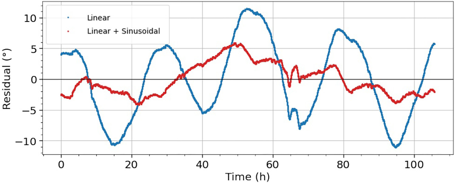
Inspection of the residuals from the linear fit, shown in Fig. 16 (blue), reveals a clear oscillatory dependence on time. The frequency $f$ determined from the linear+sinusoidal fit shown in Table 4 corresponds to a period $T=26.563\pm 0.001$ h. This value is in excellent agreement with the expected half-turn period of the pendulum, $T_{\text{th}}=26.43$ h, indicating a strong correlation between the observed modulation and the pendulum dynamics.

Figure 16
Residuals of the linear and linear+sinusoidal fits.

To compare the experimental results with the theoretical prediction given by Eq. (2), the systematic error associated with the purely linear model was estimated from the difference between the slopes of the two fits. The fitted parameters are summarized in Tables 3 and 4.

The difference between the slopes, $\Delta \text{Ω}=a^{\prime }-a={0.016}^{\circ }/h$, provides an experimental estimate of the systematic error associated with the linear fit. Taking this contribution into account, the measured precession rate is ${\text{Ω}}_{\text{1st run}}=6.79\pm {0.02}^{\circ }/h.$

When compared with the theoretical value for our latitude, ${\text{Ω}}_{\text{th}}={6.810}^{\circ }/h$, this result differs by approximately $0.30\%$. However, it should be noted that since the data is highly correlated due to the moving average, the associated uncertainties are underestimated.

In order to express a more representative value, it is useful as well to observe the angular dependence of the precession rate. Figure 17 shows the plot of $\text{Ω}\left(\phi \right)$ for two complete turns of the pendulum. The global precession rate was obtained by dividing the dataset into blocks of 1705 points (about 10 degrees of precession expected, $N=34$ blocks) and performing an ordinary least-squares linear fit of $\phi \left(t\right)$ within each block to determine the local angular velocity. This block-wise procedure was applied independently to two complete turns.

Figure 17
Blue and orange shaded bands correspond to the uncertainty of the individual turns, the black shaded band represents the statistical dispersion between turns, and the purple band indicates the total adjusted uncertainty, $\Delta {\overline{\text{Ω}}}_{\text{1st run}}=\frac{{\sigma }_{\text{Ω}}}{\sqrt{N}}$ of the global mean, ${\overline{\text{Ω}}}_{\text{1st run}}$.

The global mean and its error was determined to be ${\overline{\text{Ω}}}_{\text{1st run}}=6.8\pm 0.3{}^{\text{∘}}\text{/h}$, while the standard deviation is ${\sigma }_{\text{Ω}}=1.4{}^{\text{∘}}\text{/h}$, indicating significant dispersion. Although the relatively large value of ${\sigma }_{\text{Ω}}$ indicates a non-negligible angular dependence of the local precession rate, this systematic variation averages out in the global estimate, resulting in a mean value that agrees with the theoretical expectation within experimental uncertainty.

A similar analysis performed on other three independent data sets with different values for the amplitude, azimuth and pulling time is exhibited on Table 5.

Table 5
Summary of results.

Run	$\theta$ (∘)	${\phi }_0$ (∘)	$t_e$ (ms)	$t_p$ (ms)	$\overline{\text{Ω}}\pm \Delta \overline{\text{Ω}}$(∘/h)	${\sigma }_{\text{Ω}}$ (∘/h)	Duration (h)
1st	2.5	8.5	200	100	$6.8\pm 0.3$	1.4	104
2nd	3.6	88.0	200	200	$6.8\pm 0.3$	1.4	104
3rd	2.9	0.4	200	140	$7.0\pm 0.3$	1.1	86
4th	3.2	0.3	200	160	$7.1\pm 0.3$	1.3	99

5. Discussion

The observed dispersion in the local precession rate, ${\sigma }_{\text{Ω}}$, deserves further scrutiny. Figure 18 shows the angular dependence of the precession rate for four runs with different parameters, where it can be seen that even for different amplitudes and initial azimuths, the precession rate variation is similar. The amplitude seems to play a role in the precession rate, what would be expected since for greater amplitudes the interaction (hence the perturbations) with the Charron ring is longer, and the pulling from the electromagnet as well.

Figure 18
Angular dependence of the precession rate for four runs.

One possible source of anisotropy is the irregular shape of the bob. The Olympic throwing ball presents a variable cross-sectional area depending on the oscillation direction, which could in principle introduce a direction-dependent damping force. The maximum drag force is estimated to be $F_{\text{drag}}\approx 1.3\times {10}^{-4}$ N, which is comparable in magnitude to the Coriolis force. However, this force is predominantly radial and is therefore compensated by the electromagnet during each oscillation cycle. Even if a minor angle-dependent variation in the drag force were to introduce a slight modulation of the period or a small transverse component, the strong repeatability of the angular dependence observed across independent experimental runs (shown in Figure 18) argues against a stochastic or time-varying origin [¹⁵].

Also, it is not expected that the dominant forces that gives rise to the modulation observed is due to interaction of the permanent magnet and spurious magnetic field gradients on the laboratory or the terrestrial magnetic field. From Figure 10 it is possible to estimate the magnetic moment of the permanent magnet as $m_2\approx 5\times {10}^{-2}$ A$\cdot$m². Considering typical values of gradient of the terrestrial magnetic field as $\left|\nabla {\mathbf{B}}_E\right|\approx 5\times {10}^{-8}$ T/m, the expected force, $F_{me}=\left|m_2\nabla {\mathbf{B}}_E\right|$, would be $F_{me}\approx 2.5\times {10}^{-9}$ N. Gradients of magnetic fields from laboratory structures will not be greater than $\left|\nabla {\mathbf{B}}_{Lab}\right|\approx {10}^{-5}$ T/m, therefore it is not expected a force greater than $F_{lab}\approx {10}^{-7}$ N, a thousand times smaller than the expected Coriolis force [¹⁶].

5.1. Direction-dependent damping by theCharron ring

A misaligned Charron ring represents one of the most plausible sources of the angular-dependent precession observed in Figure 17. When the ring is not perfectly centered with respect to the suspension point, the contact between the cable and the ring becomes asymmetric: for oscillations in certain directions, the cable contacts earlier on one side and later on the opposite side, or may fail to contact entirely. This asymmetry introduces a tangential impulse at the moment of contact that varies with the azimuthal angle of the oscillation plane, effectively applying a torque that modulates the local precession rate.

As discussed in Section 2, the method employed for the construction of the Charron ring provides excellent alignment between the ring and the thread where the pin vise is attached, but it does not allow for translational adjustments, only leveling. Additionally, the 3D-printed adapter used in the Charron ring could be deformed under use or have print imperfections, and although it was carefully sanded prior to its use, no stress test was performed.

Taking these details into account, this component may be the main source of spurious precession.

5.2. Non-radial magnetic interactions

Although our analysis in Section 3 demonstrated that transverse magnetic impulses from a 1 mm misalignment are approximately two orders of magnitude smaller than the Coriolis impulse per half-cycle ($J_M/J_C\approx 0.05$), this comparison considers only a single passage. Over the course of a 104-hour experiment comprising more than 120,000 oscillations, even such small impulses could accumulate if they are systematically correlated with the oscillation direction. Several factors can break the ideal axial symmetry: the permanent magnet is not a perfect point dipole, producing higher-order multipole moments, and the electromagnet may exhibit azimuthal asymmetries due to imperfect winding or core inhomogeneities.

5.3. Airy precession

It is worth emphasizing that, even in the case of a free Foucault pendulum, there are subtleties that must be carefully addressed in order to properly describe its motion [¹⁷, ¹⁸], especially those related to the intrinsic precession of the elliptical motion of the pendulum. As an exercise, let us assume that the area $A$ of the ellipse described by the projection of the bob remains below 350 mm² (1 mm for the semi-minor axis and 100 mm for the semi-major axis). In this case, the intrinsic precession according to equation (3) would be ${\text{Ω}}_{\text{prec}}<{1.4}^{\circ }$/h (interestingly enough, the same value found for the standard deviation, ${\sigma }_{\text{Ω}}$). Since this relation holds in this form only for a free pendulum, this suggests that the combination of a carefully aligned Charron ring and a gentle release is sufficient to keep the ellipticity at acceptable levels for long-duration measurements.

One possibility for the negligible elliptical motion that should be investigated further is the magnetic attraction between the permanent magnet on the bob and the metallic enclosure of the electromagnet. Although they are at least 30 mm apart in the equilibrium position, it could be the case that the pendulum is attracted to the center in each swing, keeping the elliptical motion small. This would be similar to the method described in [¹¹], where another permanent magnet is placed right below the equilibrium point at a distance to be experimentally determined, in order to nullify any intrinsic precession. Another method to eliminate the elliptical motion is described in the work of Schumacher and Tarbet that shows how to nullify this intrinsic precession by controlling the distance at which the bob receives a push from the electromagnet [¹⁹].

6. Final Remarks

In Brazil, to the best of our knowledge, only a few Foucault pendulums have been installed and are working: two in the city of Rio de Janeiro, RJ ($\lambda ={22.1}^{\circ }$ S) and one in the city of Porto Alegre, RS ($\lambda ={30}^{\circ }$ S). Moreover, the only record of a quantitative experiment with a Foucault pendulum in Brazil was found in an article published in 1991, describing an installation in the city of São Paulo, SP ($\lambda ={23.5}^{\circ }$ S) [²⁰].

The use of an electromagnet to maintain the oscillatory motion of the pendulum is well established in the literature [²¹, ²², ²³, ²⁴]. The triggering mechanism proposed in this work, however, represents a novel approach, as it does not rely on a secondary sensor coil nor on physical contact between the pendulum cable and Charron ring to close a circuit. Instead, the $z$ component of the magnetic field, detected by a magnetic sensor, is employed to monitor the pendulum’s motion, while the $x$ and $y$ components are used to determine the angle of the oscillation plane.

The replacement of custom analog electronics with a programmable microcontroller illustrates a wider trend in instrumentation, the shift from hardware-intensive solutions to software-intensive ones, where simple sensors combined with algorithms can replace traditionally complex experimental setups [²⁵]. The Arduino and Python scripts (and the 3D parts to print as well) are available at an online repository, so that it can be built by universities, science centers, and for other educational purposes [²⁶].

In future work, we intend to review the Charron ring mechanism, refine the algorithm used and integrate the webcam into the system so that the precession rate can be quantitatively determined through image recognition techniques, similar to Ref. [²⁷], with image capture automatically managed by the microcontroller.

Appendix A: Static Test of the Permanent Magnet and Electromagnet

One of the advantages of this implementation is that several off-the-shelf components are used, making it easier to replicate the setup. One of these items is the electromagnet, which is sold with minimal specifications, only indicating a 30 kg lifting capacity and providing no information about the strength of the magnetic field or number of coils.

In order to assess its strength, the axial component of the magnetic field was measured for several distances (where zero was defined as the surface of the electromagnet). The static test used a 24 V power source and a measured current of 0.92 $\pm$ 0.01 A, the same configuration of the pendulum. The magnetic sensor (with resolution of 0.01 G) was mounted in a track and aligned with the center of the electromagnet. The sensor was then moved from a distance of 20 cm towards the electromagnet in equal intervals (with a $\pm 1\times {10}^{-4}$ m uncertainty), and the corresponding axial magnetic field was recorded. For comparison, it was also performed a similar experiment with the permanent magnet, shown in Figure 19. The fitted power laws was found to be

Figure 19
Magnetic field of the permanent magnet and the electromagnet along the z axis.

(9) $$B_{electromag}\left(z\right)=\frac{\left(1.054\pm 0.005\right)\times {10}^{-1}}{z^{1.607\pm 0.001}}$$

(10) $$B_{perm.mag}\left(z\right)=\frac{\left(1.85\pm 0.03\right)\times {10}^{-2}}{z^{1.7502\pm 0.0004}},$$

with $B$ measured in gauss and $z$ in meters.

Although the power law fitted for the magnet and electromagnet is far from a dipole approximation, an axial symmetry is expected as well.

To estimate the force between the permanent magnet and the electromagnet, a static test was performed attaching the permanent magnet to a dynamometer and varying its distance from the electromagnet along the vertical axis. The measured force (minus the magnet weight) is displayed on the vertical axis (with an uncertainty of $\pm 0.001$ N) and the adjusted curve isgiven by

(11) $$F\left(z\right)=\frac{\left(1.212\pm 0.004\right)\times {10}^{-5}}{z^{2.5806\pm 0.007}},$$

with $F$ given in newtons and $z$ in meters.

In the pendulum system, when the electromagnet is activated, the bob is near its maximum amplitude, and the distance between the bob and the top of the electromagnet is about 10 cm (note that in this case they are not axially aligned). Therefore, it would not be expected a force greater than $F_{\mathrm{mag}}\left(0.1\text{m}\right)=\left(4.6\pm 0.2\right)\times {10}^{-3}$ N, extrapolated from the fit of the graph in Figure 20.

Figure 20
Static test of the force between the permanent magnet and electromagnet along the z axis.

Acknowledgments

The authors gratefully acknowledge Eng. Alberto Costa Giesbrecht for providing the wall rack used as a support, Mr. Flávio dos Santos Jerez for his assistance in assembling and securing the system and Mr. Eder Furtado Costa for his skillful machining of the bob and the support. We also thank Prof. Daniel Alejandro Ponce Saldías and Prof. Fábio Rafael Segundo for useful discussions.

Data Availability

The entire dataset supporting the results of this study is available at the GitHub repository at the reference [²⁶].

References

• ^[1] R.P. Crease, The prism and the pendulum: the ten most beautiful experiments in science (Random House, New York, 2003).
• ^[2] W.B. Somerville, Q. J. R. Astron. Soc. 13, 40 (1972).
• ^[3] S.E. Urban and P.K. Seidelmann, Explanatory Supplement to the Astronomical Almanac (University Science Books, Mill Valley, 2013).
• ^[4] H.R. Crane, American Journal of Physics 63, 33 (1995).
• ^[5] D.B. Plewes, Review of Scientific Instruments 89, 065112 (2018).
• ^[6] G.L. Baker, Seven Tales of The Pendulum (Oxford University Press, Oxford, 2011).
• ^[7] E. Islam, Propagation: A Journal of Science Communication 1, 145 (2010).
• ^[8] N.N. Salva and H.R. Salva, American Journal of Physics 93, 297 (2025).
• ^[9] E.O. Schulz-DuBois, American Journal of Physics 38, 173 (1970).
• ^[10] M.F. Charron, L’Astronomie 45, 457 (1931).
• ^[11] H.R. Crane, American Journal of Physics 49, 1004 (1981).
• ^[12] G. Mastner, V. Vokurka, M. Maschek, E. Vogt and H.P. Kaufmann, Rev. Sci. Instrum. 55, 1533 (1984).
• ^[13] P.B. Landecker, D.D. Villani and K.W.P. Yung, Magnetic and Electrical Separation 10, 29 (1999).
• ^[14] W. Greiner, Classical Mechanics: Systems of Particles and Hamiltonian Dynamics (Springer, Berlin, 2010).
• ^[15] A.C. Longden, Phys. Rev. 13, 241 (1919).
• ^[16] J. Milsom and A. Eriksen, Field Geophysics (John Wiley & Sons, Hoboken, 2011).
• ^[17] J.A. Giacometti, Revista Brasileira de Ensino de Física 43, e20190140 (2021).
• ^[18] E.M. Diniz, Revista Brasileira de Ensino de Física 45, e20220325 (2023).
• ^[19] R.A. Schumacher and B. Tarbet, arXiv:0902.1829 (2020).
• ^[20] C.H. Furukawa and W. Sano, Revista de Ensino de Fisica 13, 2 (1991).
• ^[21] W.A. Hilton, American Journal of Physics 46, 436 (1978).
• ^[22] H. Kruglak, L. Oppliger, R. Pittet and S. Steele, American Journal of Physics 46, 438 (1978).
• ^[23] J. Priest and M.J. Pechan, American Journal of Physics 76, 188 (2008).
• ^[24] B. Lacsny, I. Štubňa and A. Teleki, European Journal of Physics 35, 065023 (2014).
• ^[25] P.A. Cotfas, D.T. Cotfas and H. Hedesiu, LabVIEW - Virtual Instrumentation in Education and Industry (IntechOpen, London, 2024).
• ^[26] E. Scatena and V.A. Cammarosano, Arduino and python scripts for drive and data acquisition of a Foucault pendulum, available at: https://github.com/escatena/foucault/
  » https://github.com/escatena/foucault/
• ^[27] D.W. Jung and K.S. Lee, J. Korean Phys. Soc. 87, 729 (2025).

Edited by

• Editor-in-Chief:
  Marcello Ferreira https://orcid.org/0000-0003-4945-3169

Publication Dates

• Publication in this collection
  31 July 2026
• Date of issue
  2026

History

• Received
  13 Mar 2026
• Reviewed
  04 May 2026
• Accepted
  07 June 2026