A rigorous derivation of the electric field on the surface of a conducting sphere

Uma dedução rigorosa do campo elétrico na superfície de uma esfera condutora

Abstract

In the paper [RBEF 42, e20200182 (2020)], I showed that the electric field on the surface of a charged conducting sphere of radius $R$ in electrostatic equilibrium evaluates to half the field discontinuity across its surface, i.e. $E_{\text{surf}}=\frac{1}{\text{2}}kQ/R^2=\frac{1}{\text{2}}\sigma /{ϵ}_0$, where $\sigma$ is the charge density on the surface. However, this exact result, found by converting an improper integral into a proper one, was criticized by Assad in a recent paper [RBEF 43, e20200467 (2021)], where he argues that this conversion would be invalid because the electric field should be undefined for points at the surface. In this work, I develop a more careful treatment of integrals and limits, which confirms our previous result within the rigour of mathematical analysis, contrarily to Assad’s arguments.

Keywords:
Electric field; Conducting sphere; Improper integrals; Integration techniques

Resumo

No artigo [RBEF 42, e20200182 (2020)], eu mostrei que o campo elétrico na superfície de uma esfera condutora carregada de raio R em equilíbrio eletrostático resulta igual à metade da descontinuidade do campo através da sua superfície, i.e. $E_{surf}=\frac{1}{\text{2}}kQ/R^2=\frac{1}{\text{2}}\sigma /{ϵ}_0$, onde σ é a densidade de carga na superfície. No entanto, esse resultado exato, obtido convertendo-se uma integral imprópria em uma própria, foi criticado por Assad em um artigo recente [RBEF 43, e20200467(2021)], onde ele argumenta que tal conversão seria inválida porque o campo elétrico deveria ser indefinido para pontos na superfície. Neste trabalho, eu desenvolvo um tratamento mais cuidadoso de integrais e limites, que confirma nosso resultado anterior dentro do rigor da análise matemática, contrariamente aos argumentos de Assad.

Palavras-chave:
Campo elétrico; Esfera condutora; Integrais impróprias; Técnicas de integração

1. Introduction

Despite the practical impossibility of building a perfectly-shaped metallic sphere of macroscopic size, the electric field due to an ideal sphere of radius $R$ and charge $Q$ in electrostatic equilibrium can, a priori, be determined mathematically. So much so that its derivation using Gauss’s law is found in introductory physics textbooks, the result being that, as the free charge in any conductor accumulates on its surface (see, e.g., Sec. 23.3 of Ref.[¹]), the field strength leaps from zero, anywhere inside the sphere, to a maximum of $Q/\left(4\pi {ϵ}_0{R}^2\right)=\sigma /{ϵ}_0$, attained just outside it (see, e.g., Sec. 23.6 in Ref. [¹] or Example 22.5 in Ref. [²]). Here, $\sigma =Q/\left(4\pi R^2\right)$ is the charge density on the surface and ${ϵ}_0$ is the vacuum electric permittivity. However, Gauss’s law is inconclusive for points located at the spherical surface because the amount of charge enclosed by the Gaussian surface is uncertain when it is chosen as the surface of the sphere itself. On noting that textbooks do not properly cover this case, in 2018 I developed a simple model to investigate it [³], in which the charge distribution is treated as a large number of thin, circular, uniformly-charged ribbons, each one with a radius $r=\sqrt{R^2-z^2}$ and charge $dQ=\sigma dA=\sigma \left(2\pi rds\right)$, where $ds=Rd\theta$ is the width of the ribbons, $\theta$ being the polar angle (in spherical coordinates), as indicated in Fig. 1. The $z$-axis is chosen along the line from the center O of the sphere, where $z=0$, to a point P at its surface, for which $z=R$. Due to azimuthal symmetry, the electric field $dE$ in P from each charged ribbon points along the $z$-axis direction, so $d\mathbf{E}=d{E}_z\widehat{\mathbf{k}}$, where $\widehat{\mathbf{k}}$ is the unit-vector for the $z$-axis. From the well-known formula for the field due to a uniformly-charged ring, as seen, e.g., in Eq. (22.4.7) of Ref. [¹], one finds [³, Eq. (14)]

(1) $$d{E}_z=k\frac{R-z}{{\left[r^2+{\left(R-z\right)}^2\right]}^{\frac{3}{\text{2}}}}dQ,$$

which holds for $-R\le z<+R$. Here, $k=1/\left(4\pi {ϵ}_0\right)$ is the Coulomb constant. After some algebra, the corresponding integral simplifies to [³, Eq. (18)]

(2) $$E_z=k\frac{Q}{4R^2\sqrt{2R}}{\int }_{-R}^{+R}\frac{1}{\sqrt{R-z}}\mathit{d}z,$$

which is an improper integral, since its integrand is not a bounded function on the entire integration interval (it has an infinite discontinuity at $z=R$).¹ There in Ref. [³], this integral was evaluated by taking the usual limit for improper integrals into account (see, e.g., Sec. 8.8 of Ref. [⁴]), which yielded²

(3) $$\begin{array}{ll}{\displaystyle {\int }_{-R}^{+R}\frac{1}{\sqrt{R-z}}dz}\hfill & =\underset{ϵ\to 0^{+}}{\lim }{\displaystyle {\int }_{-R}^{R-ϵ}\frac{1}{\sqrt{R-z}}dz}\hfill \\ \hfill & ={-2\underset{ϵ\to 0^{+}}{\lim }\sqrt{R-z}|}_{-R}^{R-ϵ}=2\sqrt{2R}.\hfill \end{array}$$

This promptly reduces Eq. (2) to

(4) $$E_z=\frac{1}{\text{2}}\frac{kQ}{R^2}=\frac{1}{\text{2}}\frac{\sigma }{{ϵ}_0},$$

as found in Eq. (20) of Ref. [³]. Therefore, this is the correct result for the electric field strength on the surface of a charged conducting sphere within the rigour of differential and integral calculus.

Figure 1
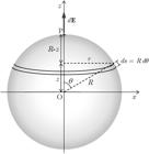
A conducting sphere with radius $R$ and charge $Q>0$, with a uniform charge density $\sigma$ on its surface, is cut into a large number of thin circular ribbons, each one with a radius $r$ and charge $dQ=\sigma \left(2\pi rds\right)$. The center of the exhibited ribbon lies at a height $z$ above the center O of the sphere and it creates an electric field $d\mathbf{E}=d{E}_z\widehat{\mathbf{k}}$ at point P.

The result in Eq. (4) was soon criticized by Assad in Ref. [⁶], where he argues that the field on the surface of a conducting sphere cannot be determined mathematically, so the evaluation of the improper integral, above, should be invalid. In his words (our emphasis),

As the electric field has a non-integrable singularity at the point of the surface where one wants to derive the field, (…) [his first reference and our Ref. [³]] make the regularization of the divergent integral by changing the upper limit of integration of the rings, which is equivalent to remove from the sum an infinitesimal element of charge at the position where one wants to derive the field, leaving a small ‘hole’ in the surface. (…) one can’t define the value of the field “on the surface”.³

Could the limit evaluation in Eq. (3) be invalid? By suspecting that this is not the case, in 2020 I did investigate how to convert that improper integral into an equivalent proper integral (i.e., a regular Riemann definite integral) [⁷]. On rewriting Eq. (1) in terms of $\theta$, one finds [⁷, Eq. (2)]

(5) $$d{E}_z=\frac{\pi }{\sqrt{2}}k\sigma \frac{\sin \theta }{\sqrt{1-\cos \theta }}d\theta .$$

As the function $\sin \theta /\sqrt{1-\cos \theta }$ is an indeterminate form of the kind ‘$0/0$’ at $\theta =0$ (which corresponds to $z=R$), one has to check its limit as $\theta \to 0^{+}$. In footnote 3 of Ref. [⁷], it is mentioned that

(6) $$\underset{\theta \to 0^{+}}{lim}\frac{\sin \theta }{\sqrt{1-\cos \theta }}=\sqrt{2}.$$

We shall prove this result in the next section. Finally, by taking into account some trigonometric identities, the integral corresponding to Eq. (5) was simplified to [⁷, Eq. (4)]

(7) $$E_z=\pi k\sigma {\int }_0^{\pi }\cos \mathrm{ }\left(\frac{\theta }{2}\right)\mathit{d}\theta ,$$

which is a proper integral, since its integrand is bounded and continuous for all $0\le \theta \le \pi$. In Ref. [⁷], this elementary integral was solved using the simple substitution $u=\theta /2$, which led to $E_z=2\pi k\sigma {\int }_0^{\pi /2}\cos udu=2\pi k\sigma =\sigma /\left(2{ϵ}_0\right)$, confirming our previous result.

However, the proper integral in Eq. (7) was also criticized by Assad in 2021, when he insisted that one could not assign any definite value to the electric field on the surface of a charged conducting sphere, so the conversion of the improper integral in Eq. (2) to the proper one in Eq. (7) should be invalid. In his words (our emphasis, our words in brackets) [⁸],

(…) the field does not become continuous at this point ($z=R$ or $\theta =0$), nor the function becomes integrable there at this point by a change of variables. The discontinuity [of the function in the integrand] is a topological invariant.”

Here in this work, I rederive the electric field on the surface of a conducting sphere following a more careful mathematical treatment of the integrals and limits in order to check the validity of the result $E_z=\sigma /\left(2{ϵ}_0\right)$within the rigour of mathematical analysis.

2. A More Rigorous Approach

Within classical electrostatics, the electric field due to a charged conducting sphere is everywhere the same as that of a uniformly-charged spherical shell with the same radius and charge, as their charge distributions are identical. Then, on treating such shell as a collection of thin circular charged ribbons, as described in the previous section, the direct integration $E_z=\int d{E}_z$ of Eq. (1) will inevitably lead to the improper integral in Eq. (2), whose integrand tends to infinity as $z\to R^{-}$. This improper integral was solved in Ref. [³] by evaluating the usual limit, which showed that $E_z=\sigma /\left(2{ϵ}_0\right)$ is the correct result within the rigour of calculus. Could a more careful, rigourous mathematical treatment lead to a different result? In what follows, we shall prove that this is not the case.

Theorem 1

Given a spherical shell with radius $R$ and electric charge $Q$ uniformly distributed on its surface, in electrostatic equilibrium, the electric field in any point at the shell is given by

$${\mathbf{E}}_{\mathrm{surf}}=\frac{1}{\text{2}}\frac{\sigma }{{ϵ}_0}\widehat{\mathbf{r}},$$

where $\sigma =Q/\left(4\pi R^2\right)$ is the areal charge density and $\widehat{\mathbf{r}}$ is the radial (outward) unit-vector at that point.

Proof.

In order to find a proper integral equivalent to the improper one in Eq. (2), namely

(8) $$I_1\equiv {\int }_{-R}^{+R}\frac{1}{\sqrt{R-z}}\mathit{d}z,$$

we begin substituting $z=R\cos \theta$, which leads to

(9) $$\begin{array}{ll}{I}_1\hfill & =R{\displaystyle {\int }_0^{\pi }\frac{\sin \theta }{\sqrt{R-R\cos \theta }}d\theta }\hfill \\ \hfill & =\sqrt{R}{\displaystyle {\int }_0^{\pi }\frac{\sin \theta }{\sqrt{1-\cos \theta }}d\theta ,}\hfill \end{array}$$

in which the integrand $f\left(\theta \right)\equiv \sin \theta /\sqrt{1-\cos \theta }$ is a continuous function on the half-open interval $(0,\pi ]$,⁴ being an indeterminate form of the kind ‘$0/0$’ at $\theta =0$. Let us then evaluate its limit as $\theta \to 0^{+}$, in order to check if it remains bounded on $(0,\pi ]$. On taking into account the technique of rationalization of the denominator, one finds that, for all $\theta \in (0,\pi ]$,

(10) $$\begin{array}{ll}f(\theta )\hfill & =\frac{\sin \theta }{\sqrt{1-\cos \theta }}=\frac{\sin \theta \cdot \sqrt{1+\cos \theta }}{\sqrt{1-\cos \theta }\cdot \sqrt{1+\cos \theta }}\hfill \\ \hfill & =\frac{\sin \theta \sqrt{1+\cos \theta }}{\sqrt{1-{\cos }^2\theta }}\hfill \\ \hfill & =\sqrt{1+\cos \theta },\hfill \end{array}$$

from which it follows that

(11) $$\underset{\theta \to 0^{+}}{lim}f\left(\theta \right)=\underset{\theta \to 0^{+}}{lim}\sqrt{1+\cos \theta }=\sqrt{2}.$$

This finite value reflects the fact that the charge $dQ=\sigma dA=\sigma \left(2\pi rds\right)=2\pi \sigma R^2\sin \theta d\theta$ of each ring tends to zero as $\theta \to 0^{+}$, otherwise (i.e., if any finite charge would be occupying the ‘last ring’) the Coulombian field at point P would tend to infinity as the distance from the ring to P tends to zero. In fact, the assumption that the ‘last ring’ shelters a finite amount of charge is false and it is the root of the incorrect reasonings developed by Assad in Refs. [⁶, ⁸]. Moreover, the finiteness of the limit above shows that the integrand $f\left(\theta \right)$ remains bounded on the half-open interval $(0,\pi ]$, so its discontinuity at $\theta =0$ is a removable one and we can securely proceed with the regularization of the integral in Eq. (9). For this, we replace the original integrand $f\left(\theta \right)$ by the piecewise function

(12) $$\tilde{f}(\theta )\equiv \{\begin{array}{ll}\sqrt{2},\hfill & \theta =0\hfill \\ \frac{\sin \theta }{\sqrt{1-\cos \theta }},\hfill & 0<\theta \le \pi \hfill \end{array},$$

which is the continuous extension of $f\left(\theta \right)$ to the closed interval $[0,\pi ]$, whose existence will be established in Eq. (24).⁵ By applying the same rationalization steps taken in Eq. (10), this new function simplifies to

(13) $$\tilde{f}\left(\theta \right)=\sqrt{1+\cos \theta },$$

which, of course, is a continuous function for all real values of $\theta$, as follows from the theorems in footnote ⁴. For a better comparison with $f\left(\theta \right)$, see Fig. 2. On substituting $\tilde{f}\left(\theta \right)$ in the integral in Eq. (9), one finds

(14) $$I_1=\sqrt{R}{\int }_0^{\pi }\sqrt{1+\cos \theta }\mathit{d}\theta ,$$

which already is a proper integral, since its integrand is bounded and continuous on the closed interval $[0,\pi ]$.⁶ The half-angle identity ${\cos }^2\left(\theta /2\right)=\left(1+\cos \theta \right)/2$, which holds for all real values of $\theta$, simplifies the integral in Eq. (14) to

(15) $$\begin{array}{ll}{I}_1\hfill & =\sqrt{R}{\displaystyle {\int }_0^{\pi }\sqrt{2}\left|\cos \left(\frac{\theta }{2}\right)\right|d\theta }\hfill \\ \hfill & =\sqrt{2R}{\displaystyle {\int }_0^{\pi }\cos \left(\frac{\theta }{2}\right)d\theta },\hfill \end{array}$$

Figure 2
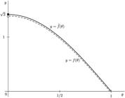
Comparison of the integrands $f\left(\theta \right)=\sin \theta /\sqrt{1-\cos \theta }$, as given in Eq. (9), and $\tilde{f}\left(\theta \right)=\sqrt{1+\cos \theta }$, as given in Eq. (13). The horizontal axis is for $\theta$ in units of $\pi$ rad. The dashed curve is for $y=f\left(\theta \right)$, which is discontinuous at $\theta =0$, where it is an indeterminate form of the kind ‘$0/0$’ (empty ball). For clarity, it has been displaced downward. Note that $f\left(\theta \right)$ tends to $\sqrt{2}$ as $\theta \to 0^{+}$, see Eq. (11). The solid curve is for $y=\tilde{f}\left(\theta \right)$, which is continuous at $\theta =0$ (black ball).

the last step being justified by the fact that $\cos \left(\theta /2\right)\ge 0$ for all $\theta ϵ[0,\pi ]$. The theorems mentioned in footnote ⁴ guarantee the continuity of the integrand $\cos \left(\theta /2\right)$ for all real values of $\theta$, which suffices for its integrability on $[0,\pi ]$. The last integral above is just the proper integral in Eq. (7), the one criticized by Assad in Ref. [⁸]. Its evaluation is easily accomplished by noting that the function $F\left(\theta \right)\equiv 2\sin \left(\theta /2\right)$ is an antiderivative of $\cos \left(\theta /2\right)$ for all $\theta$, which allows us to apply the Fundamental Theorem of Calculus.⁷ This yields

(16) $$\begin{array}{ll}{I}_1\hfill & =\sqrt{2R}\left[{2\sin \left(\frac{\theta }{2}\right)|}_0^{\pi }\right]\hfill \\ \hfill & =2\sqrt{2R}\left[\sin \left(\frac{\pi }{2}\right)-\sin 0\right]\hfill \\ \hfill & =2\sqrt{2R}.\hfill \end{array}$$

On substituting this result in Eq. (2), one finds

(17) $$E_z=k\frac{Q}{2R^2}=\frac{1}{\text{2}}\frac{\sigma }{{ϵ}_0}.$$

In order to prove this result in an even more complete and rigorous way, we must show that the last integral in Eq. (9) actually exists and is completely equivalent to the proper one in Eq. (15), beyond any doubt. Both things are justified by a strong result of mathematical analysis, our Theorem 2. For completeness, before presenting and proving it, let us give a formal definition for the Riemann integral and state some integrability conditions.

We begin defining a partition${\wp }_n^{[a,b]}$ of a real interval $[a,b]$ as any set of $n+1$ distinct points $\{x_0,x_1,\dots ,x_{n-1},x_n\}$ in which $a=x_0<x_1<\dots <x_{n-1}<x_n=b$, $n>0$ being an integer. Clearly, ${\wp }_n^{[a,b]}$ divides $[a,b]$ in $n$ subintervals $[x_{j-1},x_j]$, $j=1,\dots ,n$, each one with a length$\Delta x_j\equiv x_j-x_{j-1}>0$. A Riemann sum (1854) of $f:[a,b]\to ℝ$ over ${\wp }_n^{[a,b]}$ is any sum of the kind

(18) $$\sum _{j=1}^{n}f\left(c_j\right)\Delta x_j,$$

where $c_jϵ[x_{j-1},x_j]$ for all $j=1,\dots ,n$. The Darboux sums (1875) are the Riemann sums in which all $c_j$’s are chosen as either the infimum (i.e., the greatest lower bound) or the supremum (i.e., the least upper bound) of $f\left(x\right)$ in each subinterval. This yields, respectively, the Darboux lower sum

(19) $$ℒ\mathrm{ }(f,{\wp }_n^{[a,b]})\equiv \sum _{j=1}^n{m}_j\Delta x_j$$

and the Darboux upper sum

(20) $$𝒰\mathrm{ }(f,{\wp }_n^{[a,b]})\equiv \sum _{j=1}^n{M}_j\Delta x_j,$$

where $m_j\equiv inf\left\{f\left(x\right),x\in [x_{j-1},x_j]\right\}\le M_j\equiv sup\left\{f\left(x\right),xϵ[x_{j-1},x_j]\right\}$. The Riemann integral${\int }_a^{b}f\left(x\right)\mathit{d}x$ is then defined as the limit⁸

(21) $$\underset{\max \left\{\Delta x_j\right\}\to 0}{lim}\sum _{j=1}^{n}f\left(c_j\right)\Delta x_j=L,$$

where $c_jϵ[x_{j-1},x_j]$ for all $j=1,\dots ,n$, as long as this limit exists and belongs to $ℝ$. As a consequence of the uniqueness of limits [¹¹, Theorem 4.1.5], when this limit exists it is unique, so $L$ has to be the same, independently of the manner the $c_j$’s are chosen. In this case, we say that $f\left(x\right)$ is Riemann-integrable on $[a,b]$. Rigorously speaking, the existence of this limit means that, given any $ϵ>0$, there must be a $\delta >0$ sufficiently small, depending on $ϵ$, but not on the particular choice of the $c_j$’s, such that

(22) $$\left|{\displaystyle \sum }_{j=1}^{n}f(c_j)\mathrm{\Delta }{x}_j-L\right|<ϵ,$$

for all partitions ${\wp }_n^{[a,b]}$ with $\max \left\{\Delta x_j\right\}<\delta$. This definition becomes complete by including ${\int }_a^{a}f\left(x\right)\mathit{d}x\equiv 0$ and ${\int }_b^{a}f\left(x\right)\mathit{d}x\equiv -{\int }_a^{b}f\left(x\right)\mathit{d}x$.

As the definition of the Riemann integral involves a limit, it is important to establish some integrability conditions in order to guarantee that such limit exists – i.e., that $f\left(x\right)$ is Riemann-integrable. The most basic rule states that a function $f:[a,b]\to ℝ$ is Riemann-integrable on $[a,b]$ only if it is bounded on this interval, as proved in Theorem 3.1.2 in Ref. [¹²]. Though the boundness of the integrand is a necessary condition for Riemann integrability, it is not sufficient, as nicely illustrates the Dirichlet function $f:[0,1]\to \{0,1\}$, defined as 1 if $x$ is a rational number and 0 otherwise, for which $0\le f\left(x\right)\le 1$ for all $xϵ[0,1]$, so $f\left(x\right)$ is bounded on $[0,1]$, but it is not Riemann-integrable.⁹ In the search for an integrability criterion, the Darboux sums reveal their utility through the Darboux criterion: a bounded function $f:[a,b]\to ℝ$ is Riemann-integrable on $[a,b]$if and only if, for every $ϵ>0$, there is a partition ${\wp }_n^{[a,b]}$ such that

(23) $$\mathcal{U}\left(f,{\wp }_n^{[a,b]}\right)-ℒ\left(f,{\wp }_n^{[a,b]}\right)<ϵ\text{.}$$

For a proof of this criterion, see, e.g., Theorem 7.2.8 of Ref. [¹⁰] or Theorem 5.4 of Ref. [¹³]. As proved in Theorems 3.2.5 and 3.2.6 of Ref. [¹²], $f\left(x\right)$ is Riemann-integrable on $[a,b]$ if and only if ${\int }_a^{b}f\left(x\right)\mathit{d}x=I=S$, where $I$ is the infimum of all Darboux upper sums and $S$ is the supremum of all Darboux lower sums. In particular, the Darboux criterion allows one to prove that the continuity of a real function $f\left(x\right)$ on a closed interval $[a,b]$, with $b>a$, is a sufficient condition for its integrability, as done, e.g., in Theorem 5.10 of Sec. III.5 in Ref. [¹³]. An interesting consequence of Eq. (23) is that an isolated discontinuity does not affect the integrability of a bounded function $f:[a,b]\to ℝ$, nor the value of ${\int }_a^{b}f\left(x\right)\mathit{d}x$, as proved in Example 7.3.1 and Theorem 7.3.2 of Ref. [¹⁰]. Therefore, if $f:[a,b]\to ℝ$ has only one isolated, finite discontinuity at $x=c$, $a\le c\le b$, we can always choose

(24) $$\tilde{f}(c)=\{\begin{array}{ll}\underset{x\to c}{\lim }f(x),\hfill & \text{if}a<c<b\hfill \\ \underset{x\to a^{+}}{\lim }f(x),\hfill & \text{if}c=a\hfill \\ \underset{x\to b^{-}}{\lim }f(x),\hfill & \text{if}c=b\hfill \end{array}$$

in order to make $\tilde{f}\left(x\right)$ continuous throughout the closed interval $[a,b]$, without affecting the value of the corresponding integral (i.e., $\tilde{f}\left(x\right)$ will be the continuous extension of $f\left(x\right)$ to the closed interval $[a,b]$). The lemma below extends integrability to bounded functions with any kind of discontinuity in $[a,b]$.¹⁰

Lemma 1 (Bounded function discontinuous at one point)

Let $f:[a,b]\to ℝ$ be a function bounded on $[a,b]$ and discontinuous only at a point $cϵ[a,b]$. Then, $f\left(x\right)$ will be Riemann-integrable on $[a,b]$ and

$${\int }_a^{b}f\left(t\right)dt=\underset{x\to c^{-}}{lim}{\int }_a^{x}f\left(t\right)dt+\underset{x\to c^{+}}{lim}{\int }_x^{b}f\left(t\right)dt.$$

Incidentally, the value of ${\int }_a^{b}f\left(t\right)\mathit{d}t$ will be the same whatever be the real value attributed to $f\left(c\right)$.

Proof.

Since $f\left(x\right)$ is bounded on $[a,b]$, then there is a real $M$ such that $\left|f\left(x\right)\right|\le M$ for all $xϵ[a,b]$. Being $f\left(x\right)$ discontinuous only at $x=c$, assume $a<c<b$.¹¹ Then, given any $ϵ>0$, there is a (small) $\delta >0$ such that $M\cdot \left|x-c\right|<ϵ/4$ whenever $\left|x-c\right|<\delta$. Since $f\left(x\right)$ is bounded and continuous for all $x\ne c$, then $f\left(x\right)$ will be Riemann-integrable on both intervals $[a,d]$, where $a<d<c$, and $[e,b]$, where $c<e<b$. On taking $d=c-\delta$ and $e=c+\delta$, this means that there are two partitions ${\wp }_n^{[a,d]}$ and ${\wp }_m^{[e,b]}$ such that

(25) $$𝒰\left(f,{\wp }_n^{[a,d]}\right)-ℒ\left(f,{\wp }_n^{[a,d]}\right)<\frac{ϵ}{4}$$

and

(26) $$𝒰\left(f,{\wp }_m^{[e,b]}\right)-ℒ\left(f,{\wp }_m^{[e,b]}\right)<\frac{ϵ}{4}.$$

Once any finite value is chosen for $f\left(c\right)$, we can build a new partition ${\tilde{\wp }}_{n+m+1}^{[a,b]}$ as the union of the two previous partitions with the point $x_k=c$. For this partition,

(27) $$\begin{array}{l}𝒰\left(f,{\tilde{\wp }}_{n+m+1}^{[a,b]}\right)-ℒ\left(f,{\tilde{\wp }}_{n+m+1}^{[a,b]}\right)\le 2M\delta \hfill \\ +𝒰\left(f,{\wp }_n^{[a,d]}\right)-ℒ\left(f,{\wp }_n^{[a,d]}\right)\hfill \\ +𝒰\left(f,{\wp }_m^{[e,b]}\right)-ℒ\left(f,{\wp }_m^{[e,b]}\right)\hfill \\ <\frac{ϵ}{2}+\frac{ϵ}{4}+\frac{ϵ}{4}=ϵ.\hfill \end{array}$$

From Eq. (23), it follows that $f\left(x\right)$ is Riemann-integrable on $[a,b]$.

Finally, take into account the functions $F:[a,c]\to ℝ$, defined as $F\left(x\right)\equiv {\int }_a^{x}f\left(t\right)\mathit{d}t$, and $G:[c,b]\to ℝ$, defined as $G\left(x\right)\equiv {\int }_x^{b}f\left(t\right)\mathit{d}t$. As they both fulfill the Lipschitz condition $\left|F\left(\beta \right)-F\left(\alpha \right)\right|\le H\cdot \left|\beta -\alpha \right|$ for all $\alpha$ and $\beta$ in their respective domains,¹² they are uniformly continuous there,¹³ which means that $F\left(c\right)+G\left(c\right)=\underset{x\to c^{-}}{lim}F\left(x\right)+\underset{x\to c^{+}}{lim}G\left(x\right)$. Therefore,

(28) $$\begin{array}{l}{\displaystyle {\int }_a^{c}f(t)\mathrm{ }dt}+{\displaystyle {\int }_c^{b}f(t)\mathrm{ }dt}\hfill \\ \begin{array}{cc}& =\underset{x\to c^{-}}{\lim }{\displaystyle {\int }_a^{x}f(t)\mathrm{ }dt}+\underset{x\to c^{+}}{\lim }{\displaystyle {\int }_x^{b}f(t)\mathrm{ }dt}.\end{array}\hfill \end{array}$$

In virtue of Theorem 7.4.1 of Ref. [¹⁰], the integrability of $f\left(x\right)$ on the separate intervals $[a,c]$ and $[c,b]$ implies that ${\int }_a^{c}f\left(t\right)\mathit{d}t+{\int }_c^{b}f\left(t\right)\mathit{d}t$ necessarily has the same value of ${\int }_a^{b}f\left(t\right)\mathit{d}t$.

Although a function $f:[a,b]\to ℝ$unbounded on $[a,b]$ is not Riemann-integrable on this interval, it still can have a convergent improper integral on $[a,b]$. The intention behind the use of limits to define improper integrals certainly is to extend the result of Lemma 1 to functions unbounded at a point $cϵ[a,b]$. This is just the case of the integral for $E_z$ in our Eq. (2). In the case of functions that are undefined at a point belonging to the integration interval, as in the case of the integrand $f\left(\theta \right)$ in Eq. (9), the theorem below gives support for a similar extension.

Theorem 2 (Integral of a bounded function discontinuous at one of the endpoints)

If a function $f:(a,b]\to ℝ$ is bounded on the half-open interval $(a,b]$ and Riemann-integrable on $[c,b]$ for all $c\in (a,b)$, then it will also be Riemann-integrable on the closed interval $[a,b]$, whatever be the real value chosen for $f\left(a\right)$, and

$${\int }_a^{b}f\left(x\right)\mathrm{ }dx=\underset{c\to a^{+}}{lim}{\int }_c^{b}f\left(x\right)\mathrm{ }dx.$$

Proof.

I could find equivalent statements for this theorem in Ex. 8.4.6 of Ref. [⁵] and Ex. 1 in Sec. 3.4 of Ref. [¹²], but I could not find a formal proof in textbooks. We begin showing that, if $F:(a,b]\to ℝ$ is a decreasing function on $(a,b]$ and $F\left(x\right)\le M$ for all $x\in (a,b]$, then there is a real $L$ such that

(29) $$\underset{x\to a^{+}}{lim}F\left(x\right)=L.$$

This follows from the fact that, being the set $𝔉\equiv \left\{F\left(x\right),x\in (a,b]\right\}$ non-empty and bounded above by $M$, $𝔉$ has a supremum. Define $L\equiv sup\left\{𝔉\right\}$. Then, given any (small) $ϵ>0$, there will exist a $c\in (a,b)$, near enough to $a$, such that $L-ϵ<F\left(c\right)\le L$. The monotonicity of $F\left(x\right)$ then leads to

(30) $$L-ϵ<F\left(c\right)\le F\left(x\right)\le L,$$

for all $a<x<c$.

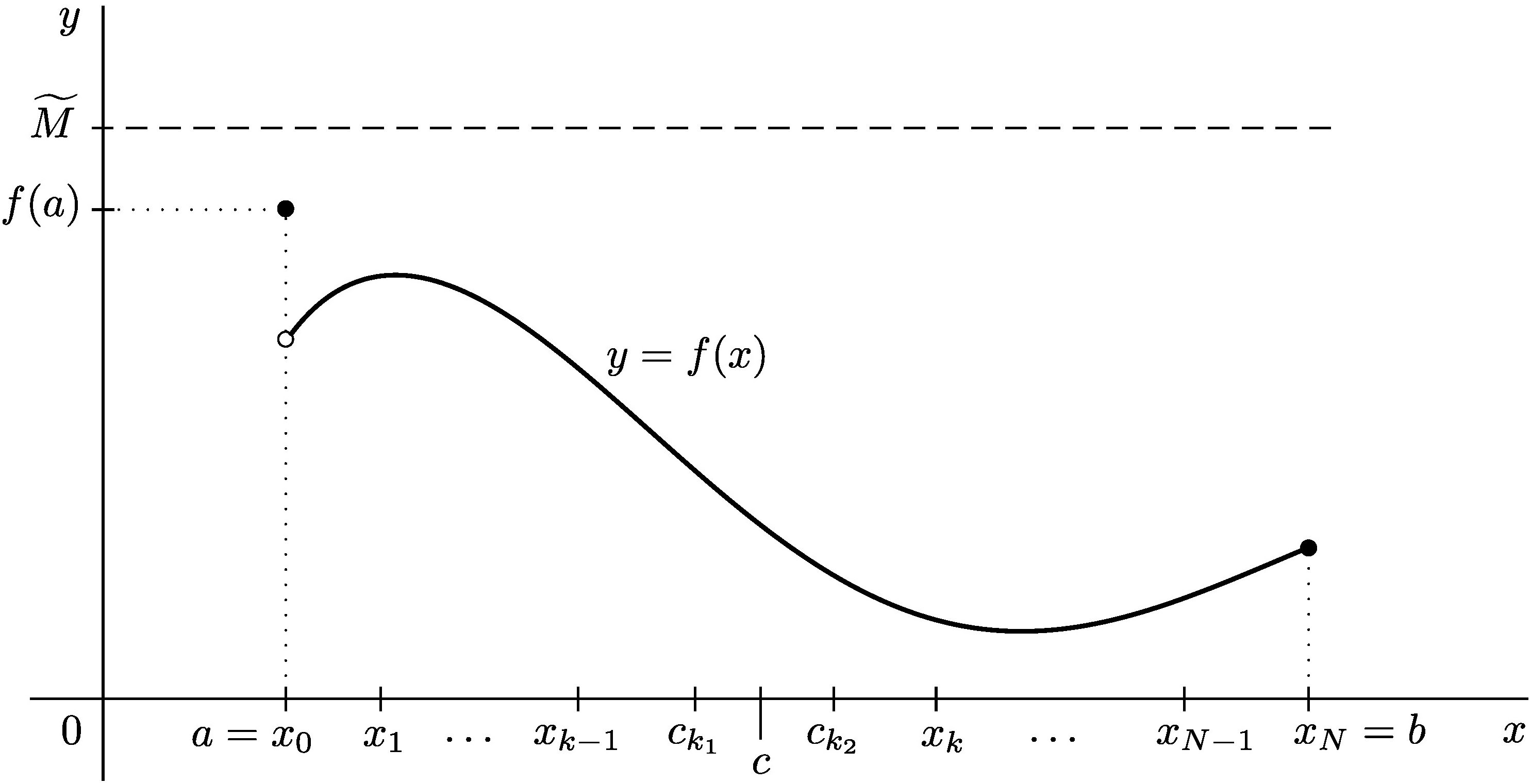
Now, let us prove that the integrability of $f\left(x\right)$ on $(a,b]$ implies its integrability on $[a,b]$. For simplicity, assume $f\left(x\right)\ge 0$ for all $xϵ[a,b]$. By hypothesis, $f\left(x\right)$ is integrable on $[c,b]$ for all $c\in (a,b)$, so we can define a function $F\left(c\right)\equiv {\int }_c^{b}f\left(x\right)\mathrm{ }dx$ for all $c\in (a,b]$. Since $f\left(x\right)\ge 0$ is bounded on $(a,b]$, it follows that $F\left(c\right)$ is a decreasing function of $c$ bounded on $(a,b]$.¹⁴ Then, according to Eq. (29), there will exist a real $L$ such that

(31) $$\underset{c\to a^{+}}{lim}F\left(c\right)=\underset{c\to a^{+}}{lim}{\int }_c^{b}f\left(x\right)\mathrm{ }dx=L.$$

Once $f\left(a\right)$ is chosen, the function $f\left(x\right)$ will be bounded on the closed interval $[a,b]$, so there will be a $\tilde{M}>0$ such that $0\le f\left(x\right)\le \tilde{M}$ for all $a\le x\le b$. This upper bound is represented by a horizontal dashed line in Fig. 3, above. The existence of the limit in Eq. (31) then means that, given an (small) $ϵ>0$, there will exist a $c\in (a,b)$, near enough to $x=a$, such that

(32) $$\left|\underset{c}{\overset{b}{{\displaystyle \int }}}f(x)\mathrm{ }dx-L\right|<\frac{ϵ}{4}.$$

Figure 3
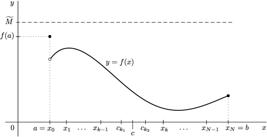
A partition ${\wp }_N^{[a,b]}$ with $\max \left\{\Delta x_j\right\}<\delta <ϵ/\left(8\tilde{M}\right)$. The positions of point $c$ and the auxiliary points $c_{k_1}$ and $c_{k_2}$ are indicated. Note that $f\left(x\right)$ is bounded above by $\tilde{M}$ and it has a finite discontinuity at $x=a$, with $0\le f\left(a\right)\le \tilde{M}$.

Of course, we can always choose $c$ such that $\tilde{M}\left(c-a\right)<ϵ/4$. Also, we can take $\delta >0$ small enough to make $2\tilde{M}\delta <ϵ/4$, and then, for any partition ${\wp }_n^{[c,b]}$ with $\max \left\{\Delta x_j\right\}<\delta$, we shall have

(33) $$\left|{\displaystyle \sum }_{j=1}^{n}f(c_j)\text{Δ}{x}_j-\underset{c}{\overset{b}{{\displaystyle \int }}}f(x)\mathrm{ }dx\right|<\frac{ϵ}{4}.$$

Analogously, for any ${\tilde{\wp }}_m^{[a,c]}$ with $\max \left\{\Delta x_j\right\}<\delta$, we shall have

(34) $$\left|{\displaystyle \sum }_{j=1}^{m}f(c_j)\text{Δ}{x}_j-0\right|<\frac{ϵ}{4}.$$

Therefore, for any partition ${\wp }_N^{[a,b]}$ with $\max \left\{\Delta x_j\right\}<\delta$, assuming that $c$ belongs to the $k$-th subinterval $[x_{k-1},x_k]$, we shall have

(35) $$\begin{array}{l}\left|{\displaystyle \sum _{j=1}^{N}f(c_j)\mathrm{\Delta }{x}_j-L}\right|\hfill \\ =\left|{\displaystyle \sum _{j=1}^{k-1}f(c_j)\mathrm{\Delta }{x}_j+f(c_k)\mathrm{\Delta }{x}_k+{\displaystyle \sum _{j=k+1}^{N}f(c_j)\mathrm{\Delta }{x}_j-L}}\right|\hfill \\ =|{\displaystyle \sum _{j=1}^{k-1}f(c_j)\mathrm{\Delta }{x}_j+f(c_{k_1})(c-x_{k-1})}\hfill \\ +{\displaystyle {\int }_c^{b}f(x)dx-L}+{\displaystyle \sum _{j=k+1}^{N}f(c_j)\mathrm{\Delta }{x}_j+f(c_{k_2})(x_k-c)}\hfill \\ -{\displaystyle {\int }_c^{b}f(x)dx}+f(c_k)\mathrm{\Delta }{x}_k\hfill \\ -f(c_{k_1})(c-x_{k-1})-f(c_{k_2})(x_k-c)|,\hfill \end{array}$$

where $c_{k_1}$ and $c_{k_2}$ also belong to the $k$-th subinterval, with $x_{k-1}\le c_{k_1}\le c\le c_{k_2}\le x_k$, as indicated in Fig. 3. The triangle inequality then yields

(36) $$\begin{array}{l}\left|{\displaystyle \sum _{j=1}^{N}f(c_j)\mathrm{\Delta }{x}_j-L}\right|\hfill \\ \le \left|{\displaystyle \sum _{j=k+1}^{N}f(c_j)\mathrm{\Delta }{x}_j+f(c_{k_2})\left(x_k-c\right)-{\displaystyle {\int }_c^{b}f\left(x\right)dx}}\right|\hfill \\ +\left|{\displaystyle {\int }_c^{b}f(x)dx-L}\right|\hfill \\ +{\displaystyle \sum _{j=1}^{k-1}f(c_j)\mathrm{\Delta }{x}_j+f(c_{k_1})(c-x_{k-1})}\hfill \\ +\left|f(c_k)\mathrm{\Delta }{x}_k-f(c_{k_1})(c-x_{k-1})-f(c_{k_2})(x_k-c)\right|\hfill \\ <\frac{ϵ}{4}+\frac{ϵ}{4}+\frac{ϵ}{4}+\frac{ϵ}{4}=ϵ.\hfill \end{array}$$

According to Eq. (22), this implies that $f\left(x\right)$ is Riemann-integrable on $[a,b]$, whatever be the real value attributed to $f\left(a\right)$. Finally, according to Eq. (31),

(37) $${\int }_a^{b}f\left(x\right)\mathit{d}x=L=\underset{c\to a^{+}}{lim}{\int }_c^{b}f\left(x\right)\mathit{d}x,$$

as we wanted to show.

The integrability of $f\left(x\right)$ on $[a,b]$ remains valid if $f\left(x\right)<0$ somewhere in $[a,b]$, but still bounded on $[a,b]$, because we can sum $f\left(x\right)$ to the absolute value of its minimum $\alpha$, so that $g\left(x\right)\equiv f\left(x\right)+\left|\alpha \right|\ge 0$ for all $xϵ[a,b]$. Then, as proved above, $g\left(x\right)$ will be integrable on $[a,b]$. On writing $f\left(x\right)=\left[f\left(x\right)+\left|\alpha \right|\right]-\left|\alpha \right|=g\left(x\right)-\left|\alpha \right|=g\left(x\right)+\left(-\left|\alpha \right|\right)$, we see that $f\left(x\right)$ is the sum of two integrable functions, so it will also be integrable on $[a,b]$, as guarantees Theorem 7.4.2(i) of Ref. [¹⁰].

Due to this theorem, it is natural to define improper integrals in which the integrand is undefined at one of the endpoints as $\underset{c\to a^{+}}{\lim }{\displaystyle {\int }_c^{b}f\left(x\right)}dx$ or $\underset{c\to b^{-}}{\lim }{\displaystyle {\int }_a^{c}f\left(x\right)}dx$. For instance, the integrand $f\left(\theta \right)=\sin \theta /\sqrt{1-\cos \theta }$ in Eq. (9) is not Riemann-integrable because it is undefined at $\theta =0$, but the function

(38) $$\tilde{f}(\theta )=\{\begin{array}{cc}f(\theta ),& \theta \ne 0\\ Y,& \theta =0\end{array}$$

is bounded and continuous on the half-open interval $(0,\pi ]$, so it is integrable on $[c,\pi ]$ for all $c\in (0,\pi )$. Then, according to Theorem 2, $\tilde{f}\left(\theta \right)$ will also be integrable on $[0,\pi ]$whatever be the real value attributed to$Y=\tilde{f}\left(0\right)$, and ${\displaystyle {\int }_0^{\pi }\tilde{f}\left(\theta \right)}d\theta =\underset{c\to 0^{+}}{\lim }{\displaystyle {\int }_c^{\pi }f\left(\theta \right)}d\theta$.¹⁵ Therefore,

(39) $$\begin{array}{ll}{I}_1\hfill & =\sqrt{R}{\displaystyle {\int }_0^{\pi }\tilde{f}(\theta )d\theta }\hfill \\ \hfill & =\sqrt{R}\underset{c\to 0^{+}}{\lim }{\displaystyle {\int }_c^{\pi }\frac{\sin \theta }{\sqrt{1-\cos \theta }}d\theta }.\hfill \end{array}$$

Now, since all rationalization steps in Eq. (10) are valid in the half-open interval $(0,\pi ]$, then

(40) $$I_1=\sqrt{R}\underset{c\to 0^{+}}{lim}{\int }_c^{\pi }\sqrt{1+\cos \theta }\mathit{d}\theta .$$

As done in Eq. (15), the half-angle identity simplifies this integral to

(41) $$\begin{array}{ll}{I}_1\hfill & =\sqrt{2R}\underset{c\to 0^{+}}{\lim }{\displaystyle {\int }_c^{\pi }\cos \left(\frac{\theta }{2}\right)d\theta }\hfill \\ \hfill & =\sqrt{2R}{\displaystyle {\int }_0^{\pi }\cos \left(\frac{\theta }{2}\right)d\theta }.\hfill \end{array}$$

This proves the equivalence between the integral in Eq. (9) and the proper integral in Eq. (15), within the rigour of mathematical analysis.

3. Conclusion

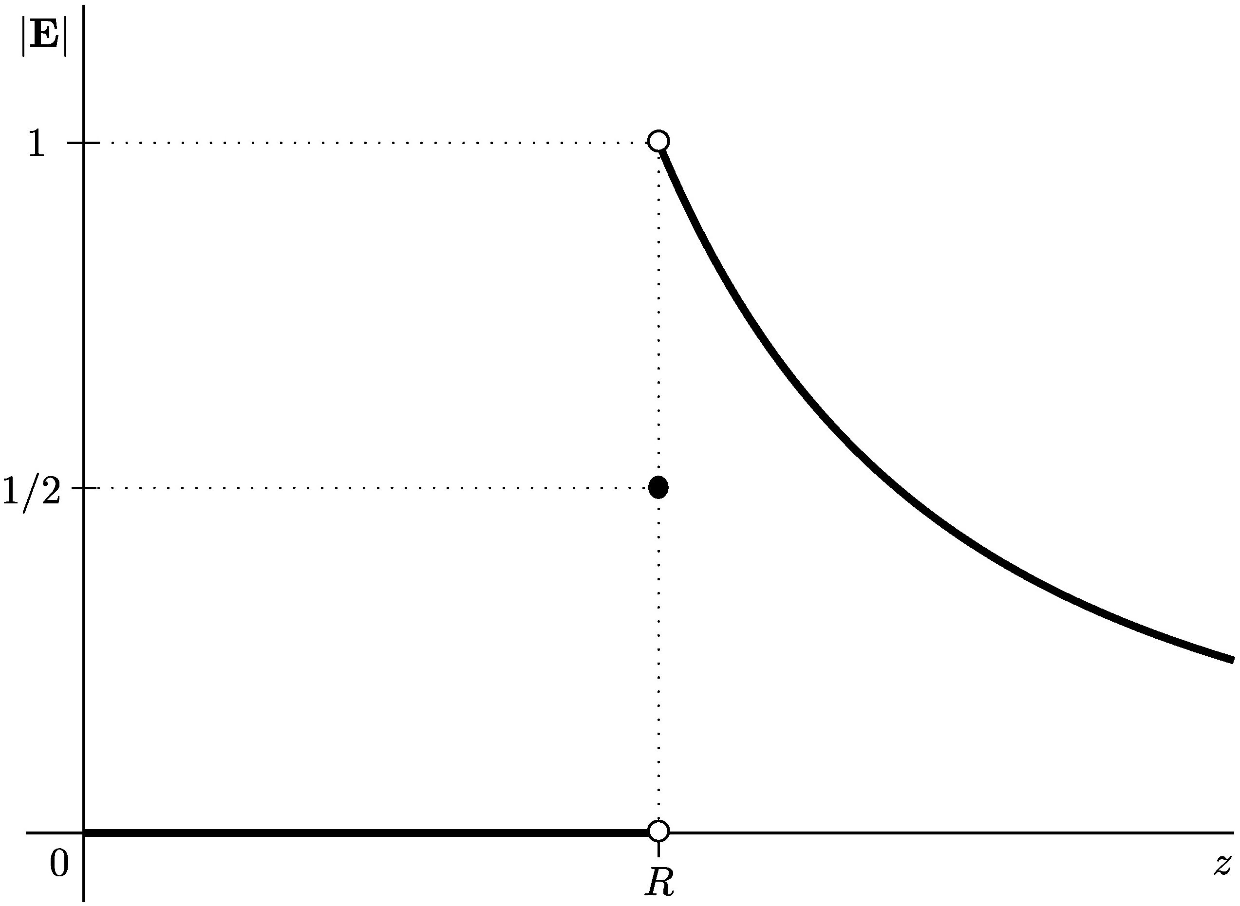
When the integrand of a given definite integral has an infinite discontinuity somewhere on its integration interval, it is unbounded and then it is not Riemann-integrable, so the corresponding integral is improper. By definition, an improper integral is convergent if the limit defining it exists in $ℝ$ [⁴, Sec. 8.8]. As proved in Ref. [³], the improper integral for the electric field on the surface of a conducting sphere of radius $R$ with a charge $Q$ in electrostatic equilibrium, as given in Eq. (2), is convergent, since its evaluation involves a limit which exists and is finite, as shown in Eq. (3). Contrarily to Assad’s view, though the value of the integrand in Eq. (2) tends to infinity as $z\to R^{-}$, the corresponding integral remains finite, its direct evaluation resulting in $E_{\mathrm{surf}}=kQ/\left(2R^2\right)=\sigma /\left(2{ϵ}_0\right)$ [³]. This is the correct result for $E_{\mathrm{surf}}$ within the rigour of calculus. Even knowing this, in Ref. [⁷] I did convert that improper integral into an equivalent proper integral in order to overcome the main Assad’s criticism in Ref. [⁶] and, as expected, this led to the same exact result. However, this alternative derivation was also disputed by Assad in Ref. [⁸], where he insisted that one could not assign any definite value to $E_{\mathrm{surf}}$, so the conversion of the improper integral in Eq. (2) to the proper one in Eq. (7) should be invalid. This has led me to develop a more careful treatment of integrals and limits, in order to check the validity of that result for $E_{\mathrm{surf}}$. As seen in the previous section, we have proved Theorem 1 following more careful mathematical steps than those in Ref. [⁷]. This showed, again, that $E_{\mathrm{surf}}=\sigma /\left(2{ϵ}_0\right)$. Even when this problem is tackled with the tools of mathematical analysis, as done in Theorem 2, the final result is the same. Therefore, the field on the surface of a conducting sphere has a definite value and the conversion of the improper integral in Eq. (2) to the proper one in Eq. (7), as done in Ref. [⁷], has been shown to be a valid mathematical procedure, contrarily to Assad’s criticism in Ref. [⁸]. The regularization of the last integral in Eq. (9) is justified by the fact that the charge $Q$ is distributed uniformly on the surface of the sphere, so the charge $dQ=2\pi \sigma R^2\sin \theta d\theta$ in each ring will tend to zero as $\theta \to 0^{+}$. This means that the ‘last ring’ encircling our point P, whose infinitesimal area is $dA=dQ/\sigma =2\pi R^2\sin \theta d\theta$, does not enclose a finite amount of charge – i.e., it cannot be treated as a finite point charge, as Assad assumed in Refs. [⁶, ⁸].¹⁶ Therefore, the singularity at $\theta =0$ in Eq. (9) is not non-integrable, contrarily to what is alleged by Assad after Eq. (3) of Ref. [⁸]. In short, the theorems proved here lead to the same previous result: the field is discontinuous on the surface, leaping from 0 to $\sigma /\left(2{ϵ}_0\right)$ when we pass from points inside the sphere to any point at its surface, and then from this value to $\sigma /{ϵ}_0$ for points just outside, as illustrated in Fig. 4.

Figure 4
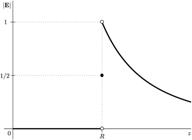
The electric field strength due to a charged conducting sphere (in units of $\sigma /{ϵ}_0$) as a function of the distance $z$ to its center. Inside the sphere of radius $R$ (i.e., for $0\le z<R$), the field is null, but at the surface (i.e., at $z=R$) it leaps to $\sigma /\left(2{ϵ}_0\right)$. For points just outside the sphere it leaps to $\sigma /{ϵ}_0$. For $z>R$, it decays proportionally to $1/z^2$.

We emphasize that it is possible to convert some improper integrals whose integrand has an infinite discontinuity at a point belonging to the integration interval (in particular, at one of the endpoints) into an equivalent proper integral. This possibility is explicitly acknowledged by Anton and co-authors in Ex. 72 of Sec. 7.8 in Ref. [¹⁴], where one reads

It is sometimes possible to convert an improper integral into a proper integral having the same value by making an appropriate substitution.

In fact, there are many examples of this conversion in textbooks, a well-known one being that of the elliptic integral that arises in the derivation of the period of a simple pendulum of length $\ell$ oscillating with angular amplitude ${\theta }_0$, namely

(42) $$T=2\sqrt{2}\sqrt{\frac{\ell }{g}}{\displaystyle {\int }_0^{{\theta }_0}\frac{1}{\sqrt{\cos \theta -\cos {\theta }_0}}d\theta },$$

where $g$ is the acceleration of gravity (see, e.g., Ex. 5 at the end of Chap. 7 in Ref. [¹⁴] or Ref. [¹⁵]). Since the above integrand tends to infinity as $\theta \to {\theta }_0^{-}$, this is an improper integral. However, the change of variables $\sin \phi =\sin \left(\theta /2\right)/\sin \left({\theta }_0/2\right)$, together with the half-angle identity $\cos \theta =1-2{\sin }^2\left(\theta /2\right)$, converts it into

(43) $$T=4\sqrt{\frac{\ell }{g}}{\int }_0^{\pi /2}\frac{1}{\sqrt{1-k^2{\sin }^2\phi }}\mathrm{ }d\phi ,$$

where $k\equiv \sin \left({\theta }_0/2\right)$. The above integral is $K\left(k\right)$, the complete elliptic integral of the first kind. Given any $0<{\theta }_0<\pi$ rad, one has $0<k^2<1$, so the integrand $1/\sqrt{1-k^2{\sin }^2\phi }$ is bounded and continuous for all $\phi ϵ[0,\pi /2]$, which makes $K\left(k\right)$ a proper integral for all $0<k<1$.¹⁷ In calculus textbooks, one finds many other examples of improper integrals that can be converted into equivalent proper integrals by applying a suitable substitution. For instance, in Ex. 72 of Sec. 7.8 of Ref. [¹⁴], the authors propose the conversion of the improper integral

(44) $$I_2\equiv {\int }_0^{\text{1}}\sqrt{\frac{1+x}{1-x}}\mathrm{ }dx$$

to a proper one by making the simple substitution $u=\sqrt{1-x}$. Since $du=-dx/\left(2\sqrt{1-x}\right)$, this change of variable leads to

(45) $$I_2=2{\int }_0^{\text{1}}\sqrt{2-u^2}\mathrm{ }du,$$

which clearly is a proper integral, since its integrand is bounded and continuous for all $uϵ[0,1]$.¹⁸ Also, in Ex. 73 of Sec. 7.8 of Ref. [¹⁴], it is proposed the conversion of the improper integral

(46) $$I_3\equiv {\int }_0^{\text{1}}\frac{\cos x}{\sqrt{x}}\mathrm{ }dx$$

to a proper integral by making the simple substitution $u=\sqrt{x}$. Since $du=dx/\left(2\sqrt{x}\right)$, one finds

(47) $$I_3=2{\int }_0^{\text{1}}\cos \mathrm{ }\left(u^2\right)\mathrm{ }du,$$

which is a proper integral, since its integrand is bounded and continuous for all $uϵ[0,1]$. All these examples definitely show that a function discontinuous at a point belonging to the integration interval can become continuous (hence, integrable) on the new integration interval by a suitable change variables, even when the discontinuity is infinite, contrarily to what is advocated by Assad in Ref. [⁸], as quoted in the end of our Sec. 1.

With respect to Assad’s opinion that the electric field has not a unique value on the surface of a charged sphere, he certainly is mistaken. If it is not unique, how many values it would have? None? An infinity? Would it be infinite (i.e., a singularity)? He does not clarify this point in Ref. [⁸]. On the other hand, our simple model developed in Ref. [³] and refined in Ref. [⁷], valid within the rigour of calculus, revealed that $E_{\mathrm{surf}}$ assumes a single, well-definite value, namely $\sigma /\left(2{ϵ}_0\right)$. Here in this work, this result has been confirmed by a more careful treatment of integrals and limits, as seen in the proof of our Theorem 1, and finally by Theorem 2, within the rigour of mathematical analysis. Therefore, the criticisms presented by Assad in Refs. [⁶] and [⁸] are unfounded, since the main result of his Eqs. (14) and (15), in Ref. [⁶], namely $\tilde{E}\left(1\right)=undefined$, is incorrect, the same occurring with Eq. (8) of Ref. [⁸]. Also, the charge $dQ$ in his Eqs. (2b) and (3b) hides an important dependence on $\theta$, without which the integration of $d{E}_z$ is non-sense. We reinforce that, though $d{E}_z$ is undefined for $z=R$ (or $\theta =0$), its integral$E_z$ (proper or improper) has a single, finite value.¹⁹

Interestingly, our result agrees with the one from a more realistic, microscopic (quantum) model, in a scale in which both the charge distribution and the electric field change continuously across the surface of a charged conductor [¹⁶, pp. 19–22]. In Fig. I.5 of Ref. [¹⁶], the electric field strength $E_n\left(x\right)$ is plotted as a function of the distance $x$ to the charged surface, according to which the field increases continuously from 0 to $\sigma /{ϵ}_0$ when we cross a thin slab of 8 Å around the surface, with $E_n\left(0\right)=0.5$ (in units of $\sigma /{ϵ}_0$). This can not be a coincidence.

In summary, though Gauss’s law yields a discontinuous electric field that leaps from 0 to $\sigma /{ϵ}_0$ when we cross the surface of a charged conducting sphere, it does not provide a definite result for the field at the surface, and certainly this is why this theme is either absent or incomplete in introductory physics textbooks. In order to give support for a better presentation of this theme in electrostatics classes and textbooks, I have shown, within the rigour of mathematical analysis, that such field actually evaluates to $\sigma /\left(2{ϵ}_0\right)$.

Acknowledgments

The author wishes to thank the (anonymous) reviewers for their recommendations, which improved the quality of this work. Thanks are also due to Mr. Isaque Ribeiro da Silva for the hints on improper integrals.

Data Availability

This work is purely theoretical and does not rely on any datasets. No data were generated or analyzed in this study.

References

• ^[1] D. Halliday, R. Resnick and J. Walker, Fundamentals of Physics (Wiley, New York, 2022), 12 ed.
• ^[2] H.D. Young and R.A. Freedman, University Physics (Pearson Education, San Francisco, 2020), 15 ed.
• ^[3] F.M.S. Lima, Resonance 22, 1215 (2018).
• ^[4] R. Larson and B. Edwards, Calculus (Cengage, Boston, 2023), 12 ed.
• ^[5] B.S. Thomson, J.B. Bruckner and A.M. Bruckner, Elementary Real Analysis (ClassicalRealAnalysis.com, 2008), 2 ed.
  » ClassicalRealAnalysis.com
• ^[6] G.E. Assad, Rev. Bras. Ens. Fís. 42, e20190245 (2020).
• ^[7] F.M.S. Lima, Rev. Bras. Ens. Fís. 42, e20200182 (2020).
• ^[8] G.E. Assad, Rev. Bras. Ens. Fís. 43, e20200467 (2021).
• ^[9] V.A. Zorich, Mathematical Analysis I (Springer, New York, 2015), 2 ed.
• ^[10] S. Abbott, Understanding Analysis (Springer, New York, 2016), 2 ed.
• ^[11] R.G. Bartle and D.R. Sherbert, Introduction to Real Analysis (Wiley, New York, 2011), 4 ed.
• ^[12] W.F. Trench, Introduction to Real Analysis (Pearson, Upper Saddle River, 2003).
• ^[13] E. Hairer and G. Wanner, Analysis by Its History (Springer, New York, 2008).
• ^[14] H. Anton, I. Bivens and S. Davis, Calculus (Wiley, New York, 2012), 10 ed.
• ^[15] F.M.S. Lima and P. Arun, Am. J. Phys. 74, 892 (2006).
• ^[16] J.D. Jackson, Classical Electrodynamics (Wiley, New York, 1999), 3 ed.

• 1
  A real function $f\left(x\right)$ is bounded on a non-empty interval $I$ if there are real numbers $m$ and $M$ such that $m\le f\left(x\right)\le M$, for all $x$ belonging to $I$. Otherwise, $f\left(x\right)$ is unbounded on $I$.
• 2
  The use of limits to evaluate improper integrals remounts to Cauchy (1823), in his lessons at the École Polytechnique [⁵, Sec. 8.4].
• 3
  In Ref. [⁶], this sentence appears below Eq. (15), whereas the last phrase appears in the second paragraph of its Sec.5.
• 4
  This is a consequence of the continuity of compositions of continuous functions (see, e.g., Theorem 1.12 of Ref. [⁴]), together the continuity of the function $\cos \theta$ for all real values of $\theta$, which is proved, e.g., in Example 4 of Ref. [⁹]. The proof for $\sin \theta$ is analogous.
• 5
  This is analogous to the regularization of ${\int }_0^{\pi }\left(\sin x/x\right)\mathit{d}x$, whose integrand is continuous on $(0,\pi ]$, but it is an indeterminate form of the kind ‘$0/0$’ at $x=0$. Since $\underset{x\to 0}{lim}\sin x/x=1$, the point $x=0$ can be ‘filled in’ by choosing $\tilde{f}\left(0\right)=1$, which makes $\tilde{f}\left(x\right)$ continuous at $\theta =0$.
• 6
  The continuity of the integrand on a closed interval implies its Riemann-integrability on this interval, as dictates Theorem 4.4 of Ref. [⁴]. This consequence of continuity is proved within the rigour of mathematical analysis in Theorem 7.2.9 of Ref. [¹⁰].
• 7
  In its usual form, this theorem reads: “If a function $f\left(x\right)$ is continuous on the closed interval $[a,b]$ and $F\left(x\right)$ is an antiderivative of $f\left(x\right)$ on $[a,b]$, i.e. $dF/dx=f\left(x\right)$ for all $xϵ[a,b]$, then ${\int }_a^{b}f\left(x\right)\mathit{d}x=F\left(b\right)-F\left(a\right)$.” See Theorem 4.9 in Ref. [⁴].
• 8
  It is redundant to indicate $n\to \infty$ in this limit, as $\max \left\{\Delta x_j\right\}\to 0$ already implies this.
• 9
  In fact, given any partition ${\wp }_n^{[0,1]}$, on choosing all $c_j$’s as irrational numbers one finds ${\sum }_{j=1}^n\left(0\times \Delta x_j\right)=0$, whereas the choice of rational values yields ${\sum }_{j=1}^n\left(1\times \Delta x_j\right)={\sum }_{j=1}^n\Delta x_j=1$. This violates the independence of the limit $L$ on the choice of the $c_j$’s.
• 10
  It is possible to extend this lemma to bounded functions with any finite number of discontinuities in $[a,b]$, and even with a countable infinite number. For those readers interested in this kind of extension, we recommend Chap. 7 of Ref. [¹⁰].
• 11
  If $c=a$ or $c=b$, the integrand $f\left(x\right)$ will admit a simple continuous extension$\tilde{f}\left(x\right)$ to $[a,b]$, as seen in Eq. (24).
• 12
  This follows from the fact that $\left|{\int }_{\alpha }^{\beta }f\left(t\right)\mathit{d}t\right|=\left|F\left(\beta \right)-F\left(\alpha \right)\right|$ is equivalent to the area under the curve $y=f\left(t\right)$ from $t=\alpha$ to $\beta$, which in turn is less than (or equal to) the area of the rectangle of basis $\left|\beta -\alpha \right|$ and height $H=\underset{[\alpha ,\beta ]}{sup}\left\{f\left(t\right)\right\}-\underset{[\alpha ,\beta ]}{inf}\left\{f\left(t\right)\right\}$.
• 13
  This uniform continuity is guaranteed by Theorem 5.4.5 in Ref. [¹¹].
• 14
  This monotonicity is better understood by interpreting $F\left(c\right)={\int }_c^{b}f\left(x\right)\mathit{d}x$ as the area below the curve $y=f\left(x\right)$, from $x=c$ to $b$.
• 15
  In particular, the choice $\tilde{f}\left(0\right)=\underset{\theta \to 0_{}^{+}}{lim}f\left(\theta \right)$, which is the continuous extension of $f\left(\theta \right)$ to $[0,\pi ]$, is perfectly valid.
• 16
  In fact, the presence of an infinitesimal charge $dQ$ at a point does not necessarily create an infinite electric field there, otherwise the well-known result for a sphere of radius $R$ with a uniform volumetric charge distribution of density $\rho =Q/\left(\frac{4}{\text{3}}\pi R^3\right)$, namely $\mathbf{E}\left(r\right)=\left(kQ/R^3\right)r\widehat{\mathbf{r}}$, valid for all $0\le r\le R$, as found, e.g., in Eq. (23.6.6) of Ref. [¹], or Example 22.9 of Ref. [²], would be wrong.
• 17
  In the limit of small amplitudes, one has $\underset{k\to 0^{+}}{lim}K\left(k\right)={\int }_0^{\pi /2}1\mathit{d}\phi =\pi /2$, which yields $T_0=2\pi \sqrt{\ell /g}$ [¹⁵].
• 18
  This definite integral is easily evaluated by substituting $v=u/\sqrt{2}$, which leads to $I_2=4{\int }_0^{1/\sqrt{2}}\sqrt{1-v^2}\mathit{d}v=4{\int }_0^{\pi /4}{\cos }^2\varphi d\varphi$, where the substitution $v=\sin \varphi$ was applied. This results in $I_2=2{\int }_0^{\pi /4}\left[1+\cos \left(2\varphi \right)\right]\mathit{d}\varphi =\pi /2+1$.
• 19
  With respect to the electric potential $V\left(z\right)$ corresponding to the electric field plotted in Fig. 4, it is a continuous function of $z$ everywhere, as given by $V\left(z\right)=kQ/R=const.,0\le z<R$ and $kQ/z,z\ge R$. However, $V\left(z\right)$ is not differentiable at $z=R$, as its lateral derivatives are distinct: the ‘left’ derivative is null, whereas the ‘right’ derivative is $-{(kQ/z^2)|}_{R^{+}}=-kQ/R^2$. This prevents us from calculating the electric field on the surface by taking the gradient of $-V\left(z\right)$ at $z=R$.

Edited by

• Editor-in-Chief:
  Marcello Ferreira https://orcid.org/0000-0003-4945-3169

Publication Dates

• Publication in this collection
  30 Mar 2026
• Date of issue
  2026

History

• Received
  07 Nov 2025
• Reviewed
  17 Feb 2026
• Accepted
  17 Feb 2026