Numerical solution of Laplace’s equation in polar coordinates by a Fourier expansion and the finite difference scheme

Abstract

The steady-state heat equation for a circular plate with Dirichlet boundary conditions has been solved using a method that combines Fourier expansion and a second-order finite difference scheme. This method is implemented in a Fortran 90 program called Laplace Solver in Polar Coordinate (LSPC). The numerical solution for a Dirichlet boundary condition with significant mathematical complexity is obtained and compared with its corresponding analytical one, showing good agreement. Furthermore, numerical solutions are obtained for two more physically realistic Dirichlet boundary conditions, where constant values are assigned over two hemispheres and four quadrants. Finally, an error analysis between the numerical and analytical solutions is performed using the error vector norm, along with a self-convergence analysis. From this, it is concluded that the method is self-convergent and exhibits a decreasing error, which depends on the number of points in the discretization for finite difference and the number of terms in Fourier expansion.

Keywords
Steady-state heat equation; Dirichlet boundary conditions; Fourier expansion; finite difference scheme

1. Introduction

The heat conduction equation is a partial differential equation, which describes the evolution of the spatial temperature distribution in a body. It can be expressed as [¹].

(1) $$\rho c_v\frac{\partial T}{\partial t}=[\nabla \cdot (k\nabla T)\mathrm{]}+q_v,$$

where ρ is the material density, c_v the specific heat capacity at constant volume, t the time, k the thermal conductivity, T the temperature and q_v the heat supplied per unit volume and time due to internal sources. For isotropic materials, the thermal conductivity is a constant. If an isotropic material, in the absence of internal heat sources (q_v = 0), is allowed to evolve for a long period of time, it reaches the steady-state, meaning that the partial time derivative becomes zero $({\partial }_{t}T=0)$. With these conditions, the heat conduction equation reduces to Laplace’s equation,

(2) $${\nabla }^{2}T=0,$$

Laplace’s equation takes different forms depending on the coordinate system chosen to study the material. In this work, a circular plate of radius R is considered (see Figure 1), which results in a two-dimensional problem, and hence polar coordinates are chosen. Therefore, Laplace’s equation for temperature T(r, θ) reads [²]

Figure 1
Schematic diagram of a circular plate of radius R, with Dirichlet boundary condition denoted by T(R, θ) = f(θ).

(3) $$\frac{{\partial }^{2}T}{\partial r^2}+\frac{1}{r}\frac{\partial T}{\partial r}+\frac{1}{r^2}\frac{{\partial }^{2}T}{\partial {\theta }^2}=0.$$

In order to solve Eq. (3), the boundary conditions (B.C.) must be specified. These conditions describe the interactions of the body with its surroundings [³]. The Dirichlet B.C. is considered in this work, which specifies the temperature distribution at the edge and is denoted by T(R, θ) = f(θ).

Although this problem has an analytical solution, this work explores an alternative numerical method for solving Laplace’s equation. This method combines a Fourier expansion and the finite difference scheme.

The following provides a general explanation of the proposed numerical method. Since the temperature function satisfies that T(r, 0) = T(r, 2π), with respect to the variable θ, it is possible to use a Fourier expansion. This expansion is substituted into Laplace’s equation, Eq. (2), which reduces the two-dimensional problem to a one-dimensional one, giving rise to a differential equation for the Fourier coefficients of the expansion, which depend only on r. Given that this equation involves first and second-order derivatives, a finite difference scheme can be applied. Subsequently, a complex linear system of equations is obtained. After an algebraic manipulation of this complex linear system, the Successive Over Relaxation (SOR) method [⁴] is used to solve the system of equations and determine the Fourier coefficients, thereby reconstructing T.

When applying the finite difference with Fourier expansion, the dimension reduction offers an advantage compared to the same method applied on a cartesian mesh for the circular geometry. This is because, in order to account for the boundary conditions, the mesh (near the boundary) needs to be modified to match the geometry. Likewise, the simple improvement of the propose method is an advantage over other methods, such as the finite element method.

2. Numerical Strategy

As mentioned at the end of the previous section, it is possible to apply a Fourier expansion to the temperature function T(r, θ) with respect to the variable θ,

(4) $$T(r,\theta )=\sum _{m=-\mathrm{\infty }}^{\mathrm{\infty }}{C}^m(r)e^{im\theta }.$$

Where the Fourier coefficient $C^m$ is, in general, a complex number and depends only on r. The index m is an integer, commonly referred to as the mode. Substituting Eq. (4) into Eq. (2) gives

(5) $$\sum _{m=-\mathrm{\infty }}^{\mathrm{\infty }}\left(\frac{d^2}{d{r}^2}{C}^m(r)+\frac{1}{r}\frac{d}{dr}{C}^m(r)-\frac{m^2}{r^2}{C}^m(r)\right)e^{im\theta }=0.$$

Since the set {exp⁡(imθ)} is linearly independent [⁵], the term in the parentheses must be zero for each mode (value of m), i.e.,

(6) $$\frac{d^2}{d{r}^2}{C}^m(r)+\frac{1}{r}\frac{d}{dr}{C}^m(r)-\frac{m^2}{r^2}{C}^m(r)=0;\forall m\in \mathrm{\mathbb{Z}.}$$

Eq. (6), which also depends on the m-mode, is a differential equation for the coefficient $C^m(r)$. To numerically solve this one-dimensional differential equation, it is necessary to discretize the radial direction. Along the radial direction, n_{r + 2} points will be taken, as shown in Figure 2. The radial discretization is from the center (r_{0 = 0}) until the edge (r = r_{nr + 1} = R) of the circular plate. The spatial step between two consecutive points r_j is h, given by R/(n_r + 1). Thus, r_j = j ⋅ h, where j = 0, 1, …, n_r, n_r + 1. For simplicity, the following notation is used, $C^m(r_j)=C_j^m$. A centered second order finite difference scheme [⁶]

Figure 2
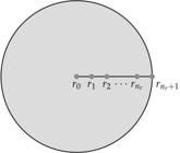
Discretization along the radial direction using n_{r + 2} points. This discretization is from the center (r_{0 = 0}) until the edge (r_{nr + 1} = R) of the circular plate.

(7) $$\frac{d}{dr}{C}_j^m=\frac{C_{j+1}^m-C_{j-1}^m}{2h},$$

(8) $$\frac{d^2}{d{r}^2}{C}_j^m=\frac{C_{j+1}^m-2C_j^m+C_{j-1}^m}{h^2},$$

is applied to all radial derivatives in Eq. (6). Reordering all the terms, it is obtain

(9) $$\begin{array}{l}\left[{\displaystyle \frac{1}{h^2}}-{\displaystyle \frac{1}{2r_{j}h}}\right]C_{j-1}^m+\left[{\displaystyle \frac{-2}{h^2}}-{\displaystyle \frac{m^2}{r_j^2}}\right]C_j^m\\ +[\frac{1}{h^2}+\frac{1}{2r_{j}h}]C_{j+1}^m=0,\forall m\in \mathbb{Z}.\end{array}$$

The last equation, for a fixed m-mode, is applied at points {r_j: j = 1, 2, …, n_r}, resulting in a underdetermined system of n_r equations with n_r + 1 unknowns $(C_0^m$, $C_1^m$,…, $C_{n_r}^m)$,

(10) $$\begin{array}{l}\begin{array}{cc}\underset{¯}{r_1}:& \left[\frac{1}{h^2}-\frac{1}{2(1h)h}\right]C_0^m+\left[\frac{-2}{h^2}-\frac{m^2}{{(1h)}^2}\right]C_1^m+\end{array}\left[\frac{1}{h^2}+\frac{1}{2(1h)h}\right]C_2^m=0,\\ \begin{array}{cc}\underset{¯}{r_2}:& \left[\frac{1}{h^2}-\frac{1}{2(2h)h}\right]C_1^m+\left[\frac{-2}{h^2}-\frac{m^2}{{(2h)}^2}\right]C_2^m+\end{array}\left[\frac{1}{h^2}+\frac{1}{2(2h)h}\right]C_3^m=0,\\ \begin{array}{ccc}& & ⋮\end{array}\\ \begin{array}{cc}\underset{¯}{r_{n_r}}:& \left[\frac{1}{h^2}-\frac{1}{2(n_{r}h)h}\right]C_{n_r-1}^m+\left[\frac{-2}{h^2}-\frac{m^2}{{(n_{r}h)}^2}\right]C_{n_r}^m+\end{array}\left[\frac{1}{h^2}+\frac{1}{2(n_{r}h)h}\right]C_{n_r+1}^m=0.\end{array}$$

Notice that the coefficient $C_{n_r+1}^m$ is evaluated at point r_nr+1, which belongs to the edge, and is obtained from the Dirichlet B.C. f(θ), by means of

(11) $$C_{n_r+1}^m=\frac{1}{2\pi }{\int }_0^{2\pi }{e}^{-im\theta }f(\theta )\mathit{d}\theta .$$

This coefficient will be integrated numerically using the composite (multiple) Simpson’s 1/3 rule for a fixed mode [⁶].

Then, to obtain a consistent system, an additional equation is required. For this, it is considered a numerical approximation where the temperature at the center is a temperature average around the center. Due to the smoothing nature of Laplace’s solution, it is possible to assume that the temperature field is locally smooth. Therefore, temperature at the center should be close to the surrounding values, in this case the temperatures at points with radius r₁. In general, the number of temperatures used for this average is arbitrary, but for simplicity, four equidistant points can be chosen to ensure they are properly distributed around the center. Thus, it is possible to establish an additional relationship between the coefficients $C_0^m$ and $C_1^m$, which allows the system, Eq. (10), to become consistent. This relationship is derived by considering the value of T(r₀, θ) = T₀ as the average temperature of four nearest neighbor points (see Figure 3).

Figure 3
Four nearest neighboring points, considered in the average for the computation of T(r₀, θ).

For this particular case, the following temperature values will be considered: T(P₁) = T₁, T(P₂) = T₂, T(P₃) = T₃ and T(P₄) = T₄. Thus, it follows that

(12) $$T_0=\frac{1}{\text{4}}(T_1+T_2+T_3+T_4)$$

(13) $${\displaystyle \sum }_{m=-\infty }^{\infty }{C}_0^m{e}^{im\theta }={\displaystyle \sum }_{m=-\infty }^{\infty }\frac{1}{\text{4}}\left(1+e^{im\pi /2}+e^{im\pi }+e^{im3\pi /2}\right)C_1^m{e}^{im\theta }$$

(14) $$4C_0^m=\underset{{\alpha }_m}{\underbrace{\left(1+e^{im\frac{\pi }{2}}+e^{im\pi }+e^{im\frac{3\pi }{2}}\right)}}{C}_1^m$$

(15) $$4C_0^m={\alpha }_m{C}_1^m.$$

Where the value of α_m depends on m-mode

(16) $${\alpha }_m\{\begin{array}{cc}4;& m\mathrm{m}\text{o}\mathrm{d}4=0\\ 0;& m\mathrm{m}\text{o}\mathrm{d}4\ne 0.\end{array}$$

Eq. (15), together with the system in Eq. (10), completes a consistent system of equations. Ordering the equations, the system obtained for a fixed m-mode (m ∈ ℤ) reads

(17) $$Az=b,$$

where,

(18) $$A=\left[\begin{array}{ccccc}4& -{\alpha }_m& 0& \dots & 0\\ \frac{1}{h^2}-\frac{1}{2h^2}& \frac{-2}{h^2}-\frac{m^2}{h^2}& \frac{1}{h^2}\text{+}\frac{\text{1}}{{\text{2h}}^{\text{2}}}& \dots & 0\\ 0& \frac{1}{h^2}-\frac{1}{4h^2}& \frac{-2}{h^2}-\frac{m^2}{4h^2}& \dots & 0\\ ⋮& ⋮& ⋮& \ddots & ⋮\\ 0& 0& 0& \cdots & \frac{-2}{h^2}-\frac{m^2}{{(n_{r}h)}^2}\end{array}\right],$$

(19) $$z^T=\left[\begin{array}{c}\hfill C_0^m{C}_1^m\mathrm{\dots }{C}_{n_r}^m\hfill \end{array}\right],$$

(20) $$b^T=\left[\begin{array}{cccc}0& 0& \dots & \left(\frac{-1}{h^2}-\frac{1}{2n_r{h}^2}\right)C_{n_r+1}^m\end{array}\right].$$

By solving the linear system, Eq. (17), it would be sufficient to substitute the solution into Eq. (4). However, it is possible to reduce the computation just for m ≥ 0. Since T(r, θ) is a real function, then it can be shown that $C_j^{-m}=C_j^{m*}$. Now, Eq. (4) is restated as follows,

(21) $$T(r_j,\theta )=C_j^0+\sum _{m=1}^{\mathrm{\infty }}(C_j^m{e}^{im\theta }+C_j^{m*}{e}^{-im\theta }).$$

For computational reasons, the summation of Eq. (21) cannot be evaluated for an infinite number of modes. Then it is necessary to truncate this summation for m until a prescribed value m_max,

(22) $$T(r_j,\theta )=C_j^0+\sum _{m=1}^{m_{max}}(C_j^m{e}^{im\theta }+C_j^{m*}{e}^{-im\theta }).$$

In this way, the number of systems to be solved is limited. After solving the system, Eq. (17), for m = 0, 1, …, m_max, the obtained coefficients are substituted into Eq. (22), in order to recover T(r_j, θ).

3. Results

In the previous section, it was shown that the temperature at certain points of the circular plate can be determined using Eq. (22), where the coefficients $\{C_j^m\}$ (m = 0, …, m_max and j = 0, …, n_r) are obtained by solving the system in Eq. (17). It should be noted that this system of equations is complex. In appendix A, an algorithm to solve such a system is described. This algorithm is based on the idea that the matrix A, as well as the vectors z and b, can be split into real and imaginary parts. The numerical strategy and the solution of the complex linear system are implemented in a Fortran 90 program called Laplace Solver in Polar Coordinates (LSPC), which is available on GitHub [⁷].

To present a solution, a boundary condition with significant mathematical complexity is proposed, which will evaluate the accuracy and stability of the method. Thus, the Dirichlet boundary condition considered, for θ expressed in radians, is given by

(23) $$f_D(\theta )=(1+{\theta }^2)\sin {\theta }^{°}C.$$

When running the LSPC program to obtain the numerical solution, it is necessary to specify the parameters defined in the method (n_r and m_max). For each pair of provided values a solution is obtained, which can be graphically represented as a heat map¹, as shown in Figure 4, for a circular plate of radius R = 1 m.

Figure 4
Heat map for the numerical solution of Laplace’s equation in polar coordinates with the Dirichlet B.C. f_D(θ), on a circular plate of radius R = 1. Considering a value of m_max = 5 and different values of n_r = 3, 7, 15, 30; with a discretization of 100 points in the variable θ to plot.

Subsequently, the numerical solution will be compare with the analytical one, which is obtained using the method of separation of variables. When the method is applied, a general solution is obtained [⁸],

(24) $$T(r,\theta )=\frac{c_0}{2}+\sum _{n=1}^{\mathrm{\infty }}{r}^n(c_n\cos n\theta +d_n\sin n\theta ).$$

Where c_n and d_n are constants, that can be determined from the Dirichlet B.C., T(R, θ) = f(θ). By multiplying the Eq. (24) by cos ⁡n′θ or sin ⁡n′θ, and integrating term-by-term over the variable θ from 0 to 2π, the equations for the coefficients c_n and d_n are obtained [⁹]. This results in,

(25) $$\begin{array}{cc}{R}^n{c}_n& =\frac{1}{\pi }{\displaystyle {\int }_0^{2\pi }f}(\theta )\cos n\theta d\theta ,n=0,1,2,\dots ;\end{array}$$

(26) $$\begin{array}{cc}{R}^n{d}_n& =\frac{1}{\pi }{\displaystyle {\int }_0^{2\pi }f}(\theta )\sin n\theta d\theta ,n=1,2,3,\dots .\end{array}$$

Thus, the analytical solution for the Dirichlet B.C. f_D(θ) is given by (see appendix B),

(27) $$T(r,\theta )=-2\pi +r\left(-\pi \cos (\theta )+\left({\displaystyle \frac{3+8{\pi }^2}{6}}\right)\sin (\theta )\right)\mathrm{}+{\displaystyle \sum _{n=2}^{\mathrm{\infty }}}{r}^n\left({\displaystyle \frac{4\pi }{n^2-1}}\cos (n\theta )+{\displaystyle \frac{8n}{{(1-n^2)}^2}}\sin (n\theta )\right).$$

This analytical solution, Eq. (27), provides the temperature at each point of the circular plate. It is represented as a heat map, as shown in Figure 5, for a circular plate with a radius of R = 1 m. From this, it can be observed that the numerical solution exhibits a good agreement with the analytical one.

Figure 5
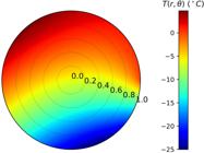
Heat map for the analytical solution of Laplace’s equation in polar coordinates with the Dirichlet B.C. f_D(θ), on a circular plate of radius R = 1.

In addition to the solution for this boundary condition f_D(θ) (which is purely mathematical), two more physically realistic cases will be presented. These cases correspond to Dirichlet boundary conditions with constant values over two hemispheres and four quadrants.

Figure 6 shows the heat map of the numerical solution obtained using the LSPC program for the following Dirichlet B.C.,

Figure 6
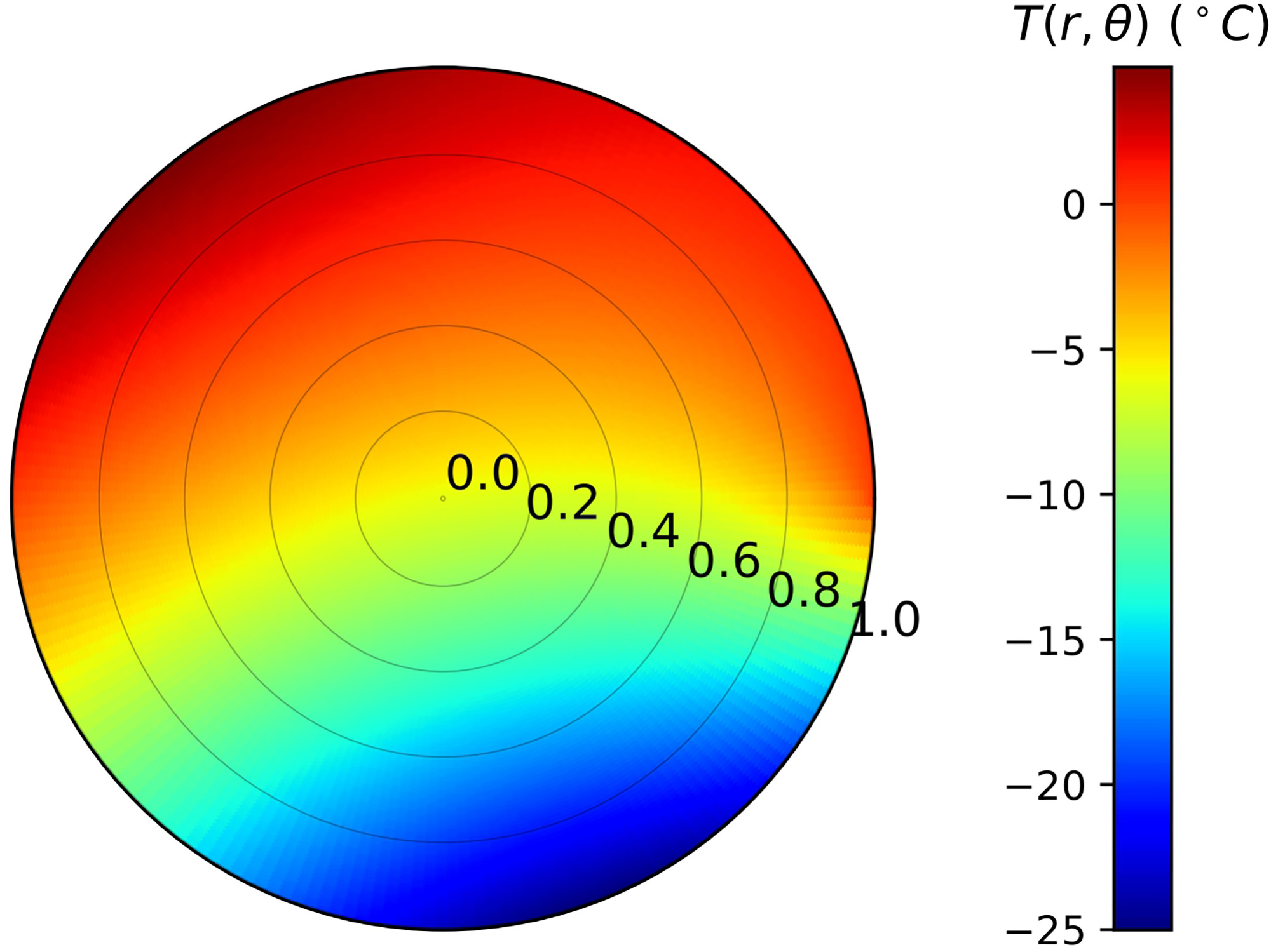
Heat map for the numerical solution of Laplace’s equation in polar coordinates with the Dirichlet B.C. f_D1(θ), on a circular plate of radius R = 1. Considering a value of m_max = 5 and n_{r = 30}; with a discretization of 100 points in the variable θ to plot.

(28) $$f_{D1}(\theta )=\{\begin{array}{cc}\hfill {20}^{°}C;\hfill & \hfill 0\le \theta <\pi \hfill \\ \hfill {10}^{°}C;\hfill & \hfill \pi \le \theta <2\pi .\hfill \end{array}$$

Figure 7 shows the heat map of the numerical solution obtained using the LSPC program for the following Dirichlet B.C.,

Figure 7
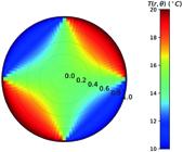
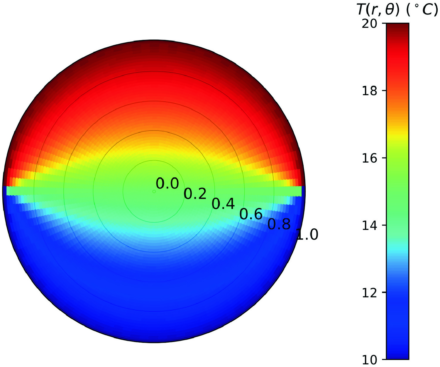
Heat map for the numerical solution of Laplace’s equation in polar coordinates with the Dirichlet B.C. f_D2(θ), on a circular plate of radius R = 1. Considering a value of m_max = 5 and n_{r = 30}; with a discretization of 100 points in the variable θ to plot.

(29) $$f_{D2}(\theta )=\{\begin{array}{cc}\hfill {20}^{°}C;\hfill & \hfill 0\le \theta <\frac{\pi }{2}\hfill \\ \hfill {10}^{°}C;\hfill & \hfill \frac{\pi }{2}\le \theta <\pi \hfill \\ \hfill {20}^{°}C;\hfill & \hfill \pi \le \theta <\frac{3\pi }{2}\hfill \\ \hfill {10}^{°}C;\hfill & \hfill \frac{3\pi }{2}\le \theta <2\pi .\hfill \end{array}$$

4. Error Analysis

In the previous section, heat maps for the boundary condition f_D were presented, showing the numerical and analytical solutions (Figure 4 and 5, respectively). Despite the good agreement between both solutions, it is possible to analyze how closely the numerical solution approaches the analytical one. Therefore, the difference between these solutions can be quantified, and this quantification will depend on the n_r and m_max parameters. To achieve this, it is necessary to define the analytical solution vector U and the numerical solution vector u. The components of U and u, correspond to the values of the analytical and numerical solution at the discretized points of the domain, respectively. Thus, the components of the error vector e = [e₁, e₂, …, e_N] (where N is the number of points in the discretization of domain) are defined by e_i = U_i − u_i. The 1-norm of the error vector [¹⁰] can be computed as follows,

(30) $$||e||=\frac{1}{N}\sum _{i=1}^N|e_i|.$$

The 1-norm quantifies the error between the analytical and numerical solution. Figure 8 shows the error vector norm as a function of the m_max parameter, keeping the n_r parameter fixed. It can be observed that for values of n_r in the range from 10 to 20, the norm does not decrease completely. In the range n_r ∈ [30, 100], the norm decreases linearly on a logarithmic scale (by simple inspection) up to a value of m_max around 40. This behavior is characteristic of methods that use a Fourier expansion and is known in the literature as spectral convergence [¹¹]. For higher m_max values, the norm increases. Finally, in the range n_r ∈ [200, 300], the norm also decreases up to a value of m_max about 40, but this decrease does not follow the linear trend observed in the previous range. It can be concluded that the range of parameters where the error decreases linearly is n_r ∈ [30, 100] and m_max ∈ [10, 40]. Then taking the error vector norms in the specified range of m_max, for a fixed value of n_r (within its specified range), it is possible to fit the norm value to [¹²]

Figure 8
Calculation of the error vector norms as a function of the parameter m_max, for different values of n_r. The graph is plotted on a logarithm scale.

(31) $$\parallel e\parallel =a\cdot e^{s\ln (m_{max})},$$

where a and s are constants. Taking the natural logarithm on both sides of equation, a linear fit on ln-ln scale (logarithm scale) is obtained, which is

(32) $$\ln (\parallel e\parallel )=s\cdot \ln (m_{max})+\ln (a).$$

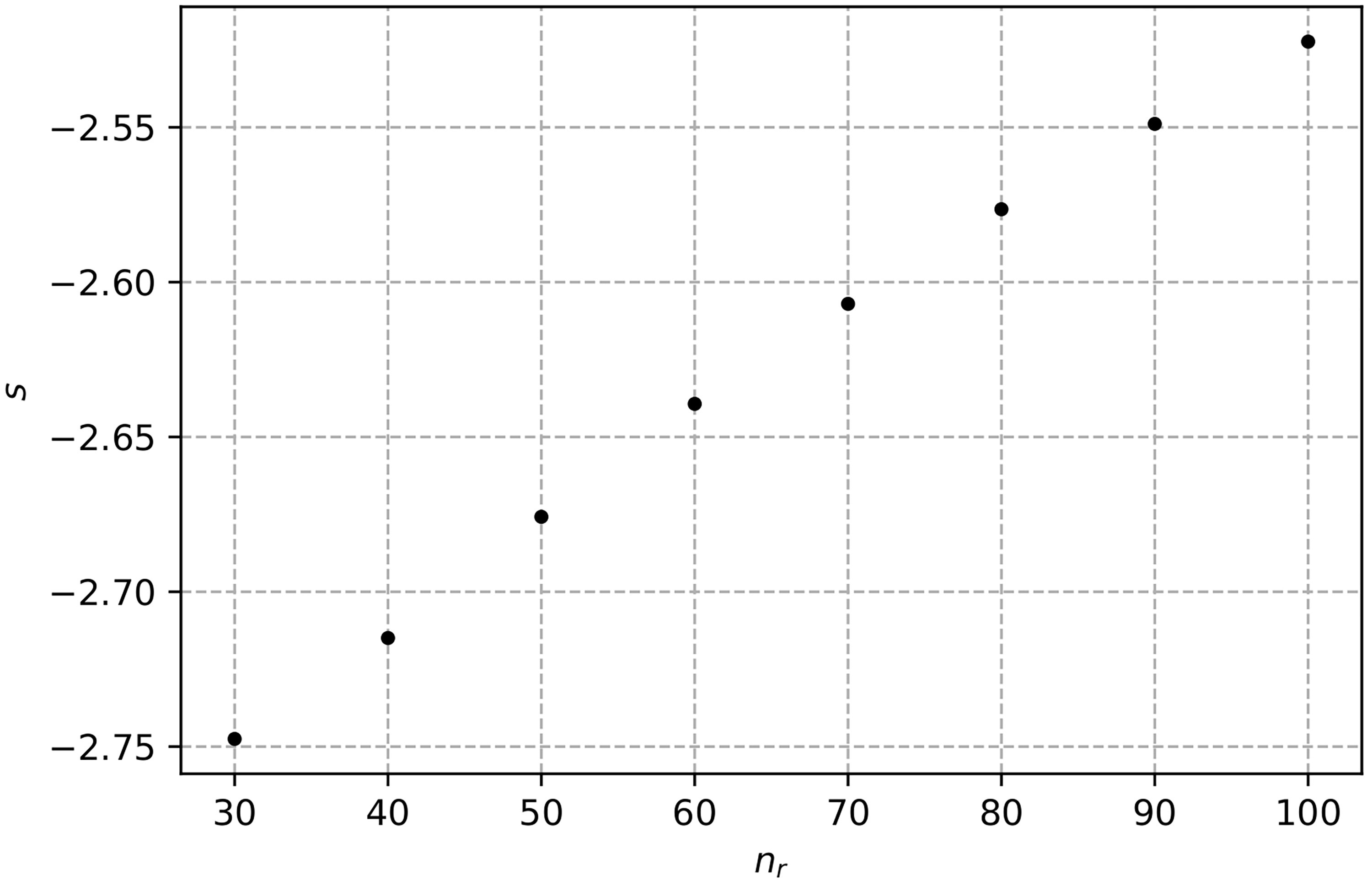
The exponent s, in Eq. (32), represents the slope of a straight line that relates the error vector norm logarithm to the logarithm of m_max value. Thus, a straight-line fit is obtained, with its respective value of s, for each n_r parameter value (see Figure 9). As show in Figure 9, s increases as n_r increases. However, since the value of s is negative, an increase in s results in a less steep line. Therefore, as the n_r value increases, the error vector norm decreases more slowly as a function of m_max. Thus, it is not very useful to consider higher values of n_r, since even with the highest value of m_max (within the range), the error would not decrease significantly.

Figure 9
The value of s as a function of n_r, obtained after fitting the error vector norm to a ⋅ exp⁡ (s ln⁡(m_max)). The error vector norms are calculated by varying m_max from 10 to 40, for a fixed value of n_r.

As mentioned, it is not useful to consider large values of n_r; for this reason, an analysis of the error vector norm as a function of h is presented in Figure 10. The parameter m_max is kept constant and fixed at 40. The aim is to analyze the range of n_r in which the expected second-order convergence of the finite difference method is attained. The range of values for the parameter m_max corresponds to the interval in which the error exhibits spectral convergence, characteristic of Fourier expansion, as shown in Figure 8. As shown in Figure 10, a set (or range) of n_r values in which the error vector norm decreases according to the fit performed with the same data (0.1724 ⋅ h^2.2630 − 0.0078 ⋅ h^1.2630 + 0.0002). The fit exhibits a second order approximately for the range n_r ∈ [10, 40]. However, Figure 8 shows that in the range n_r ∈ [10, 20] the norm stabilizes quickly, and no improvement in the approximation is obtained by increasing the value of m_max. Therefore, the range is reduced to a single value, yielding an optimal value of n_{r = 30}.

Figure 10
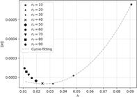
Calculation of the error vector norms as a function of h (directly related to the parameter n_r), for a fixed value of m_max equal to 40.

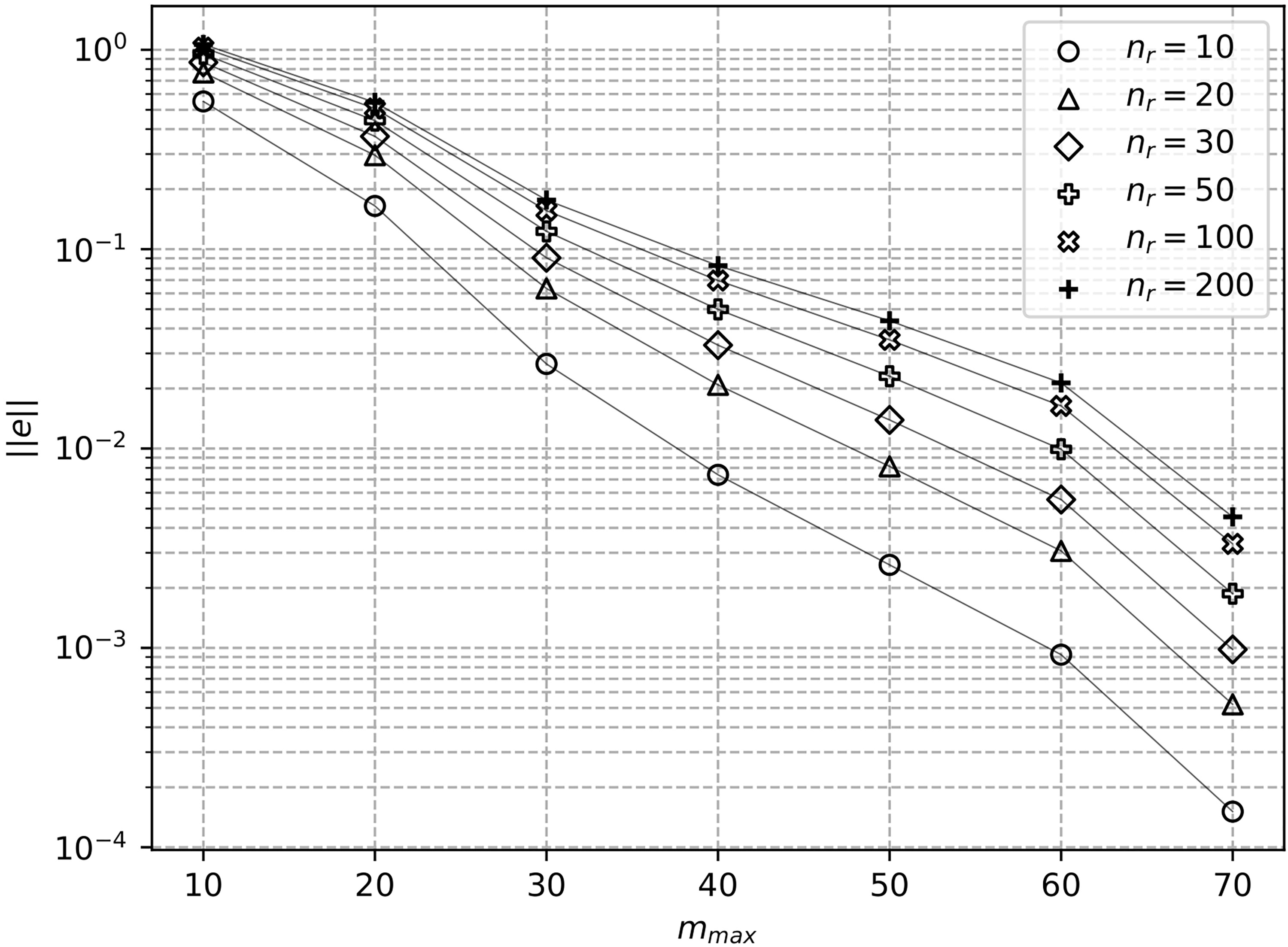
In addition to the comparison between the numerical and analytical solutions, performing a self-convergence analysis is also important. This is achieved by comparing the numerical solution itself under variations of m_max and n_r. To this end, two numerical solution vectors, $U^m$ and $U^{m^{\prime }}$, are defined, where m and m′ (m′ < m) represent the values of m_max for each solution, considering the same n_r value. The components of these vectors correspond to the numerical solution values at the discretized domain points. Thus, the new error vector is defined as $e^m=U^m-U^{m^{\prime }}$. In this case, the infinity norm of the error vector is used, which is computed as $\mathrm{|}\text{|}{e}^m\mathrm{|}{\mathrm{|}}_{\infty }=\max \left|e_i\right|$, where e_i are the components of $e^m$. Figure 11 illustrates how the error norm varies as m_max increases while keeping n_r constant. It is observed that the error decreases as m_max increases for different values of n_r. This confirms that the method is self-convergent.

Figure 11
Norm of the error vector as m_max increases, for different values of n_r. Logarithmic scale is used to plot norms.

Considering all the points discussed in this section, the range of values of the parameters n_r and m_max, where the method is self-convergent and exhibits a bounded error reduction, is given in Table 1.

Table 1
Range of values for the parameters n_r and m_max, where the method, implemented in the LSPC program, is self-convergent and presents a bounded and appropriately decreasing error.

Parameters	Range
nr	30
m max	10 - 40

5. Conclusions

This paper explores an alternative numerical method based on a Fourier expansion combined with a second-order finite difference scheme to solve the steady-state heat equation (Laplace’s equation) with Dirichlet boundary conditions on a unitary circular plate. The method was implemented in the LSPC program, which depends on the n_r and m_max parameters, which allows to compute the temperature values at the points of the discretized domain. In section 3, a numerical and analytical solution are presented, and a qualitative comparison shows them to be similar. In order to obtain a quantitative comparison, an error analysis was performed. From that, it can be concluded that the method developed and implemented in the LSPC program demonstrates self-convergence and bounded error reduction within the prescribed parameter ranges.

Among the possible extensions or modifications to the proposed method, other boundary conditions such as Neumann or mixed conditions can be considered. These types of boundary conditions specify the value of the heat flux at the boundary. In such cases, the formulation of the method would be similar up to the point of obtaining the Fourier coefficient corresponding to the boundary, since this coefficient represents the Fourier expansion of the temperature, while in these cases the flux (or both) is prescribed. Therefore, a relationship between the Fourier coefficients of the flux and the temperature would need to be established in order to obtain a consistent linear system. This would allow the calculation of the Fourier coefficients and subsequently the temperature.

Acknowledgement

Al Vicerrectorado de Investigación de la Universidad Nacional de Ingeniería, Lima, Perú.

Data Availability

The dataset supporting the results of this study is not publicly available. The dataset has been generated with the LSPC program which is available on GitHub [⁷].

Appendix

A. Complex linear system

It is possible obtain a real linear system from a complex linear system. For this, Ref. [¹³] is used. Consider a linear system

(A.1) $$Az=b,$$

where A ∈ ℂ^n×n and z, b ∈ ℂⁿ. The system can be rewritten with real matrices like

(A.2) $$(M+iN)(x+iy)=b_1+i{b}_2,$$

where M, N ∈ ℝ^n×n and x, y, b₁, b₂ ∈ ℝⁿ. After performing the operations, results

(A.3) $$Mx+iMy+iNx+i^{2}Ny=\mathrm{}{b}_1+i{b}_2$$

(A.4) $$(Mx-Ny)+i(Nx+My)=\mathrm{}{b}_1+i{b}_2.$$

Equating the real and imaginary parts of both sides of equation yields the following system

(A.5) $$\{\begin{array}{cc}\hfill Mx-Ny=\hfill & \hfill b_1\hfill \\ \hfill Nx+My=\hfill & \hfill b_2.\hfill \end{array}$$

This can be expressed in matrix form as

(A.6) $$\left[\begin{array}{cc}\hfill M\hfill & \hfill -N\hfill \\ \hfill N\hfill & \hfill M\hfill \end{array}\right]\left[\begin{array}{c}\hfill x\hfill \\ \hfill y\hfill \end{array}\right]=\left[\begin{array}{c}\hfill b_1\hfill \\ \hfill b_2\hfill \end{array}\right].$$

Finally, a real linear system that is equivalent to Eq. (A.1) is obtained. In this work, the new linear system is numerically solved using the SOR method [⁴].

B. Calculation of integrals

In this appendix, the results of the computations required to obtain the coefficients c_n and d_n of the analytical solution to Laplace’s equation, Eq. (24), are presented. The results are obtained for the boundary condition f_D, Eq. (23), from Eq. (25) and Eq. (26).

Coefficient c₀,

(B.1) $$c_0={\displaystyle \frac{1}{\pi }}{\displaystyle {\int }_0^{2\pi }}(1+{\theta }^2)\sin \theta d\theta ,$$

(B.2) $$c_0=-4\pi .$$

Coefficient c₁,

(B.3) $$c_1={\displaystyle \frac{1}{\pi }}{\displaystyle {\int }_0^{2\pi }}(1+{\theta }^2)\sin \theta \cos \theta d\theta ,$$

(B.4) $$c_1=-\pi .$$

Coefficient c_n, for n ≥ 2,

(B.5) $$c_n={\displaystyle \frac{1}{\pi }}{\displaystyle {\int }_0^{2\pi }}(1+{\theta }^2)\sin \theta \cos n\theta d\theta ,$$

(B.6) $$c_n={\displaystyle \frac{4\pi }{n^2-1}}.$$

Coefficient d₁,

(B.7) $$d_1={\displaystyle \frac{1}{\pi }}{\displaystyle {\int }_0^{2\pi }}(1+{\theta }^2){\sin }^2\theta d\theta ,$$

(B.8) $$d_1={\displaystyle \frac{3+8{\pi }^2}{6}}.$$

Coefficient d_n, for n ≥ 2,

(B.9) $$d_n={\displaystyle \frac{1}{\pi }}{\displaystyle {\int }_0^{2\pi }}(1+{\theta }^2)\sin \theta \sin n\theta d\theta ,$$

(B.10) $$d_n={\displaystyle \frac{8n}{{(1-n^2)}^2}}.$$

To evaluate the previously introduced integrals, the following relations are used

(B.11) $$\begin{array}{l}{\displaystyle \int \sin n\theta \cos m\theta d\theta }\\ ={\displaystyle \frac{m\sin m\theta \sin n\theta +n\cos m\theta \cos n\theta }{m^2-n^2}},\end{array}$$

(B.12) $$\begin{array}{l}{\displaystyle \int \sin n\theta \sin m\theta d\theta }\\ ={\displaystyle \frac{n\sin m\theta \cos n\theta -m\cos m\theta \sin n\theta }{m^2-n^2}},\end{array}$$

(B.13) $$\begin{array}{l}{\displaystyle \int \cos n\theta \cos m\theta d\theta }\\ ={\displaystyle \frac{m\sin m\theta \cos n\theta -n\cos m\theta \sin n\theta }{m^2-n^2}}.\end{array}$$

References

• ^[1] T.L. Bergman and A.S. Lavine, Fundamentals of heat and mass transfer (John Wiley & Sons, Hoboken, 2011), 7 ed.
• ^[2] G.B. Arfken, H.J. Weber and F.E. Harris, Mathematical methods for physicists: a comprehensive guide (Elsevier Science, Oxford, 2012), 7 ed.
• ^[3] D.W. Hahn and M.N. Özisik, Heat conduction (Wiley, Hoboken, 2012), 3 ed.
• ^[4] R.L. Burden, J.D. Faires and A.M. Burden, Numerical analysis (Cengage Learning, Boston, 2015), 10 ed.
• ^[5] E.M. Stein and R. Shakarchi, Fourier analysis: an introduction (Princeton University Press, Princeton, 2011).
• ^[6] S.C. Chapra and R.P. Canale, Métodos numéricos para ingenieros (McGraw-Hill, Madrid, 2015), 7 ed.
• ^[7] J. Carreño, LSPC, available in: https://github.com/JeanCLR/LSPC.
  » https://github.com/JeanCLR/LSPC.
• ^[8] W.E. Boyce and R.C. DiPrima, Elementary differential equations and boundary value problems (Wiley, Hoboken, 2012), 10 ed.
• ^[9] E.C. Titchmarsh, Introduction to the theory of Fourier integrals (Clarendon Press, Oxford, 1948), 2 ed.
• ^[10] R.J. LeVeque, Finite difference methods for ordinary and partial differential equations: steady-state and time-dependent problems (Society for Industrial and Applied Mathematics – SIAM, Philadelphia, 2007).
• ^[11] C. Canuto, M.Y. Hussaini, A. Quarteroni and T.A. Zang, Spectral methods: fundamentals in single domains (Springer, Berlin, 2006).
• ^[12] J.P. Boyd, Chebyshev and Fourier spectral methods (Dover Publications, New York, 2001), 2 ed.
• ^[13] V. Edalatpour, D. Hezari and D. Khojasteh, Mathematical Communications 20, 37 (2015).

• 1
  The Matplotlib library in Python was used to generate the heat maps and other graphics. This code can be found in the repository.

Edited by

• Editor-in-Chief:
  Marcello Ferreira https://orcid.org/0000-0003-4945-3169

Publication Dates

• Publication in this collection
  05 Dec 2025
• Date of issue
  2025

History

• Received
  07 June 2025
• Reviewed
  22 Sept 2025
• Accepted
  30 Oct 2025