Exchange regime of the spin waves in two-dimensional honeycomb-like ferromagnetic lattices

Abstract

The role of exchange interactions in the dynamics of collective excitations in magnetic materials is of essential importance, and since the experimental discovery of planar ferromagnetism, a flurry of research has rapidly reshaped the field of 2D materials. Although this topic has been widely addressed, the direct effects of exchange interactions on controlling the energy distribution of ferromagnetic systems, via the dispersion relationship, have not been adequately explored. This work investigates this theme and analyzes the repercussions on the magnonic density of states and energy fluctuations in the high symmetry paths of a ferromagnetic lattice with honeycomb topology, which made it possible to determine the points and direction most sensitive to this type of interaction.

Keywords
Spin Waves; Two Dimensional Magnetic Systems; Honeycomb Lattices

1. Introduction

The discovery of spin was one of the achievements of quantum mechanics, which, together with the Pauli exclusion principle, allowed a more fruitful understanding of the origin of magnetism in materials [¹] and a lot off applications such as nuclear magnetic ressonance (NMR) [², ³]. The study on the NMR culminated in the discovery of spin waves conceived by Felix Bloch, in 1930, as low-energy excitations above the ferromagnetic ground state [⁴].

Since its proposition, several theoretical works have investigated the propagation of magnetic excitations in ferromagnetic and antiferromagnetic systems [⁵,⁶,⁷,⁸,⁹,¹⁰,¹¹], until its experimental confirmation by Fleury in 1966 [¹²]. More recent research investigates several scenarios where new configurations point to promising applications [¹³, [¹⁴, ¹⁵]. Other works indicates that atomic doping and adsorption techniques have stimulated magnetic behaviors in two-dimensional honeycomb [¹⁶, ¹⁷] and hexagonal [¹⁸] topologies. This fact encourages the investigation of these excitations in nanostructures with this geometry in reduced dimensions, enabling important technological applications such as magnetic waveguides and magnetic memories [¹⁹]. The propagation of spin waves can be mapped in reciprocal space through the associated Goldstone bosons, the magnons. The dynamics of these quasi-particles allows the calculation of properties such as magnetic susceptibility [²⁰], demagnetization process [²¹], among others.

The honeycomb topology gained notoriety due to the discovery of graphene, which was theoretically proposed by Wallace in 1947 [²²] and obtained through the micromechanical exfoliation method of graphite by Novoselov and Geim [²³]. Since then, many studies have explored the electronic properties of graphene, leading to the discovery of its zero-gap semiconductor behavior [²⁴], among other applications in electronics [²⁵, ²⁶]. Given the induction of magnetism in these nanostructures, some research explores similar properties, such as the formation of spin valves [²⁷] and magnetoresistance [²⁸].

The present work investigated the effects of second-neighbor exchange interactions on regulating the energy of magnetic ordered states above the ground state in low temperature regimes in a two-dimensional ferromagnetic lattice with honeycomb topology, Figure 1(a). The starting point is to obtain the dispersion relation of the model, through which we investigated the influence of exchange interactions of second neighbors normalized by the interactions of first neighbors, for different regions of the reciprocal space. 2D and 3D energy maps were shown for specific values of fraction (J₂/J₁) as well as the direct influence of J₂ on the energy at both the center and the edge from the Brillouin Zone (BZ). We study the density of states under the influence of J₂ to observe at which frequencies we have the greatest number of excited magnons. Finally, the energy intensity for different values of J₂ and the energy variation in high symmetry paths were estimated. In Figure 1(a), each vertex is a magnetic ion due to the presence of an unpaired electron.

Figure 1
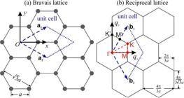
The honeycomb lattice representation (a) as a Direct lattice and (b) as a Reciprocal lattice.

2. The Hamiltonian

The Hamiltonian can be written as Eq. (1) where J₁ and J₂ are exchange terms between nearest and next-nearest neighbors, respectively. In addition, we set $h_0=H_A+g{\mu }_B{H}_0$ with H_A being the anisotropic term, g the gyromagnetic factor, μ_B the Bohr magneton and H₀ the magnetic field. Here we adopted the magnetic field in the Oz direction.

(1) $$H=-J_1{\displaystyle \sum _{\langle ij\rangle }{S}_i}\cdot S_j-J_2{\displaystyle \sum _{\langle \langle ij\rangle \rangle }{S}_i}\cdot S_j-h_0{\displaystyle \sum _i{S}_i^z},$$

The hamiltonian of the Eq. (1) can be rewritten as in Eq. (2)

(2) $$H=\frac{1}{2}{H}^{(a)}+\frac{1}{2}{H}^{(b)}+\frac{1}{2}{H}^{(I)},$$

where we define

(3)$$H^{(I)}=-J_1{\displaystyle \sum _{\langle ij\rangle }{S}_i^{(a)}}\cdot S_j^{(b)}$$

(4) $$H^{(a)}=-\frac{J_2}{2}{\displaystyle \sum _{\langle \langle ij\rangle \rangle }{S}_i^{(a)}}\cdot S_j^{(a)}-h_0{S}_i^{z(a)}$$

(5) $$H^{(b)}=-\frac{J_2}{2}{\displaystyle \sum _{\langle \langle ij\rangle \rangle }{S}_i^{(b)}}\cdot S_j^{(b)}-h_0{S}_i^{z(b)}$$

In the Eqs. (3–5) we identify $H^{(a)}$ relates to sites-a, $H^{(b)}$ to sites-b and $H^{(I)}$ to interaction factor intersites. In addition, the symbols $⟨⟩$ and $⟨⟨⟩⟩$ represent nearest and next-nearest neighbors, respectively. In the honeycomb lattice, we can count three first neighbors with distances a and six second neighbors with distances $\sqrt{3}a$, for each magnetic ion, with a being the lattice parameter, see Figure 1(a).

As was said previously, the thermal regime adopted in this work implies that $(T\ll T_C)$, where the magnetic modes have free dynamics, without inter-magnons interactions. Given this choice, we adopted the $(2S\gg a^{†}a)$ approximation in the Holstein-Primakoff transformations (HPT) [⁶]. From equations (3–5), we can write the dot products as in Eq. (6)

(6) $$S_i^{a(b)}\cdot S_j^{a(b)}=S_i^{xa(b)}{S}_j^{xa(b)}+S_i^{ya(b)}{S}_j^{ya(b)}+S_i^{za(b)}{S}_j^{za(b)}$$

and the intersite interactions are given by Eq. (7)

(7) $$S_i^a\cdot S_j^b=S_i^{xa}{S}_j^{xb}+S_i^{ya}{S}_j^{yb}+S_i^{za}{S}_j^{zb}$$

with the application of the thermal regime, the connection between the spin and bosonic operators, via HPT, is given by the Eqs. (8)

(8) $$\begin{array}{c}{S}_i^x=\frac{\sqrt{2S}}{2}(a_i+a_i^{†})\\ S_i^y=i\frac{\sqrt{2S}}{2}(a_i^{†}-a_i)\\ S_i^z=S-a_i^{†}{a}_i\end{array}$$

where S is a multiplicative constant that represents the total spin of the system with $a_i^{†}$ and a_i being creation and annihilation operators, respectively. Therefore, replacing Eqs. (8) in Eqs. (6) and (7) we obtain for Eqs. (6) the following result, Eq. (9).

(9) $$\begin{array}{c}{S}_i^a\cdot S_j^a=2S(a_i^{†}{a}_j-a_i^{†}{a}_i)\\ S_i^b\cdot S_j^b=2S(b_i^{†}{b}_j-b_i^{†}{b}_i)\end{array}$$

In addiction, the product parcels of Eq. (7) yield the Eqs. (10).

(10) $$\begin{array}{c}{S}_i^{xa}{S}_j^{xb}=\frac{S}{2}(a_i+a_i^{†})(b_j+b_j^{†})\\ \mathrm{}=\frac{S}{2}(a_i{b}_j+a_i{b}_j^{†}+a_i^{†}{b}_j+a_i^{†}{b}_j^{†})\\ S_i^{ya}{S}_j^{yb}\mathrm{}=-\frac{S}{2}(a_i^{†}-a_i)(b_j^{†}-b_j)\\ \mathrm{}=\frac{S}{2}(a_i{b}_j^{†}+a_i^{†}{b}_j-a_i{b}_j-a_i^{†}{b}_j^{†})\\ S_i^{za}{S}_j^{zb}=(S-a_i^{†}{a}_i)(S-b_j^{†}{b}_j)\\ \mathrm{}=-S(a_i^{†}{a}_i+b_j^{†}{b}_j)\end{array}$$

The Eq. (7) becomes as

(11) $$S_i^a\cdot S_j^b=S(a_i{b}_j^{†}+a_i^{†}{b}_j-a_i^{†}{a}_i-b_j^{†}{b}_j)$$

Finally, substituting Eqs. (9), (11) into Eqs. (3–5), we rewrite the Hamiltonian (2) as

(12) $$\begin{array}{cc}H& =\frac{S}{2}{\displaystyle \sum _{ij}\{}[2J_{ij}^{(1)}+J_{ij}^{(2)}+{\overline{h}}_0]{\delta }_{ij}-J_{ij}^{(2)}\}{a}_i^{†}{a}_j\\ & +\frac{S}{2}{\displaystyle \sum _{ij}\{}[2J_{ij}^{(1)}+J_{ij}^{(2)}+{\overline{h}}_0]{\delta }_{ij}-J_{ij}^{(2)}\}{b}_i^{†}{b}_j\\ & \mathrm{}-S{\displaystyle \sum _{ij}{J}_{ij}^{(1)}}(a_i^{†}{b}_j+a_i{b}_j^{†}\hfill \end{array}$$

where ${\overline{h}}_0=h_0/S$

3. Magnons Dynamics in Reciprocal Space

The propagation of spin waves in the direct lattice can be mapped by the dynamics of magnons in the reciprocal lattice. For this we apply the Fourier transform, Eq. (13), in the Eq. (12) where we find the diagonalized Hamiltonian, Eq. (14)

(13)$$a_i={\displaystyle \sum _q{e}^{iq\cdot r_i}}{a}_q$$

(14)$$H={\displaystyle \sum _q[}A(q)a_q^{†}{a}_q+B(q)b_q^{†}{b}_q+C(q)a_q^{†}{b}_q+D(q)a_q{b}_q^{†}]]$$

amplitudes are given bellow

1. $A(q)=\frac{S}{2}\left[6J_1+6J_2+{\overline{h}}_0-J_2(q)\right]$

2. $B(q)=A(q)$

3. $C(q)=-S{J}_1(q)$

4. $D(q)=C^{*}(q)$

The Eq. (14) can alternatively be expressed as

(15) $$H={\displaystyle \sum _q\left(\begin{array}{cc}{a}_q^{†}& b_q^{†}\end{array}\right)}M(q)\left(\begin{array}{c}{a}_q\\ b_q\end{array}\right)$$

with M(q) being given by

(16) $$M(q)=\left(\begin{array}{cc}A(q)& C(q)\\ D(q)& B(q)\end{array}\right)$$

or yet, $\mathbf{M}(\mathbf{q})=d^{(0)}\mathbb{𝟙}+d^{(i)}{\sigma }_i$, where $i=(1,2)$, $\mathbb{𝟙}$ and $\sigma$ assuming to be the identity matrix 2 × 2 and Pauli matrices, respectively. The d parameters assume

$$d^{(0)}=3S(J_1+J_2)+\frac{S}{2}({\overline{h}}_0-J_2(q));$$

$$d^{(1)}=JS{\displaystyle \sum _{i=1}^3\cos }(q\cdot r_i);$$

$$d^{(2)}=-JS{\displaystyle \sum _{i=1}^3\sin }(q\cdot r_i);$$

Observing the interactions between sites up to second neighbors, the structure factors become

(17)$$J_1(q)=J_1[e^{i{q}_{x}a}+e^{i(-q_x\frac{a}{2}+\frac{\sqrt{3}}{2}{q}_{y}a)}+e^{i(-q_x\frac{a}{2}-\frac{\sqrt{3}}{2}{q}_{y}a)}]$$

and

(18) $$\begin{array}{l}{J}_2(q)=J_2[e^{i(3q_x\frac{a}{2}+\frac{\sqrt{3}}{2}{q}_{y}a)}+e^{i(3q_x\frac{a}{2}-\frac{\sqrt{3}}{2}{q}_{y}a)}\\ \mathrm{}+e^{i(-3q_x\frac{a}{2}+\frac{\sqrt{3}}{2}{q}_{y}a)}+e^{i(-3q_x\frac{a}{2}-\frac{\sqrt{3}}{2}{q}_{y}a)}\\ \mathrm{}+e^{i\sqrt{3}{q}_{y}a}+e^{-i\sqrt{3}{q}_{y}a}]\end{array}$$

We can compact the geometric terms as shown in Eqs. (19) and (20).

(19)$$J_1(q)=J_1\left[\exp (i{q}_{x}a)+2\exp \left(-i{q}_x\frac{a}{2}\right)\times \cos \left(\sqrt{3}{q}_y\frac{a}{2}\right)\right]$$

(20) $$J_2(q)=J_2\left[4\cos \left(3q_x\frac{a}{2}\right)\cos \left(\sqrt{3}{q}_y\frac{a}{2}\right)+\cos (\sqrt{3}{q}_{y}a)\right]$$

Applying the Heisenberg equation, $i\mathrm{\hslash }\frac{dG}{dt}=[G,H]$, to the bosonic operators G, i.e. $G=(a,b)$, and the albegra that govern the model, $[a,a^{†}]=[b,b^{†}]=i\mathrm{\hslash }{\delta }_{q,q^{\prime }}$, $[a,b]=\mathrm{\dots }=[a^{†},b^{†}]=0$, we obtaing

(21) $$\omega G={\displaystyle \sum _{q^{\prime }}(}A(q^{\prime })[G,a_{q^{\prime }}{a}_{q^{\prime }}^{†}]+C(q^{\prime })[G,b_{q^{\prime }}{a}_{q^{\prime }}^{†}])$$

therefore, the equations of motion for operators are given in Eqs. (22)

(22) $$\begin{array}{l}\omega a_q=A(q)a_q+C(q)b_q\\ \omega b_q=D(q)a_q+B(q)b_q\end{array}$$

Solving the pair of Eqs. (22) we find the dispersion relation associated with a periodic propagation of magnetic modes, see Eq. (23).

(23) $$\omega (q)=A(q)+\sqrt{C(q)C^{*}(q)}$$

where $C(q)C^{\ast }(q)$ is given by Eq. (24)

(24) $$\begin{array}{l}C(q)C^{*}(q)=J_1^2\left[1+4{\cos }^2\left(\frac{\sqrt{3}a{q}_y}{2}\right)++4\cos \left(\frac{\sqrt{3}a{q}_y}{2}\right)\cos \left(\frac{\sqrt{3}a{q}_x}{2}\right)\right]\end{array}$$

4. Results and Methods

4.1. Results and discussions

From Eq. (23) we obtain the energy maps of the system as shown in Figure 2, that is, it reveals the energy fluctuations throughout the all BZ in the reciprocal space, see Figure 1(b), with the influence of the fitting of the term exchange of second neighbors (J₂). Here the energy growth is indicated from the blue to red. In the panel (a) shows the energy behavior considering $J_1\gg J_2$, viz the intensity of J₂ is insignificant when compared to J₁. From this panel we observe the formation of cone-like energy patterns around the K points, similar to Dirac cones in graphene, associated with the predominance of topological effects over the quadratic dependence of the magnon dispersion relation in first order, i.e. the pattern of the Dirac cone around the K points is not related to the electric or magnetic nature of the system, but to the geometry of the lattice. Furthermore, in the central region of the BZ ($\mathrm{\Gamma }$ – point), the energy maps are parabolic, circular contour lines around the point $(0,0)$, with a dominates of the red color, indicating the formation of a magnonic spectral band with greater energy concentration. The panels (b), (c) and (d) reveal the contributions of exchange interactions of neighboring seconds in gradual percentages of 10%, 20% and 30%, respectively. In panel (b), $J_2=0.1J_1$, we see the preservation of the cone-like pattern at points K, which is clear in Figure 3(b), where we draw six contour lines. However, in the central region of the BZ there is an increase in the radius of the contour curve, preserving the red color tone and the parabolicity of the dispersion relationship, resulting in a sharp variation of the energy at points of high symmetry located at the edge of the BZ, being more intense at point K, which can be perceived by the coalescence effect around this point. This behavior becomes more evident when adjusting J₂ to more expressive percentages, which is justified by the electrostatic nature of the exchange interactions that govern the bond between the magnetic sites as a response to the superposition of electronic orbitals.

Figure 2
The contour plot of the SW energy of a honeycomb ferromagnetic lattice for different interaction values of second neighbors (J₂) in percentage of first neighbors (J₁). In the upper panels (a) isolated first neighbor interaction, and in panel (b) second neighbor interaction at 10% of J₁. In the lower panels (c) and (d) we show percentages of 20% J₁ and 30% J₁, respectively.

Figure 3
3D contour plot of the SW energy of a honeycomb ferromagnetic lattice for different interaction values of second neighbors (J₂) in percentage of first neighbors (J₁). In the upper panels (a) isolated first neighbor interaction, and in panel (b) second neighbor interaction at 10% of J₁. In the lower panels (c) and (d) we show percentages of 20% J₁ and 30% J₁, respectively.

Figure 4 shows the energy map with direct dependence on J₂, which allows greater precision in measurements of the contributions of this interaction. We adopted the normalization of J₂ in terms of J₁ in order to emphasize only the variation of energy as a function of the dimensionless parameter $(J_2/J_1)$. The painels (a) and (b) show the energy behavior in the q_y direction, while in panels (c) and (d) in the q_x direction. A general aspect in all panels is the broadening of the spectral range proportional to the intensity of J₂ at all points of energy variation. We see from panel (a), where $q_y=0$, that J₂ mainly affects the modes at $q_x=2\pi /3a$, which exactly locates the high symmetry point M = $\frac{2\pi }{3a}(1,0)$, region close to the edge of the BZ, called the exchange region. This is in agreement with the energy evolution for these coordinates given the increase in J₂ observed in Figure 2. We draw attenction to the fact that no energy variation at the $\mathrm{\Gamma }$ = $\frac{2\pi }{3a}(0,0)$ point, which reflects an insensitivity of the magnetostatic region to the J₂ fluctuation. This fact is common among some traditional lattices in literature, such as square and triangular lattices. However, recent work points to the possibility of topologically extending the exchange interaction, making its effects noticeable in the region of small wave vectors in the BZ, as a result of the arrangement of magnetic sites in the lattice [²⁹]. In panel (b), where we assume $q_y=\pi /a$, we show the energy fluctuation around the high symmetry points $K=\frac{2\pi }{3a}(1,\frac{1}{\sqrt{3}})$. Here the energy variation is more sensitive when compared to panel (a), which is clear given the greater color variation, implying an additional level curve. This fact is justified by the observed region being close to the points with the highest energy response of the honeycomb lattice. The lower panels of Figure 4 reveals the energy fluctuations that are very different from each other. This is associated with the anisotropic effects of the armchair and zigzag directions on the energy variation of the magnetic modes as a function of J₂. Growthing J₂ increases energy levels but allows for a more modest rate of change, which is evident in panel d of Figs. 2 and 3.

Figure 4
The contour plot of the SW energy honeycomb-like ferromagnetic lattice as direct function of the values of second neighbors (J₂) for fix values of wave vectors. Panel a. $q_y=0$, panel b. $q_y=\frac{\pi }{a}$, panel c. $q_x=0$ and panel d. $q_x=\frac{\pi }{a}$.

Figure 5 shows the energy behavior around the high symmetry points of the lattice, see Figure 1(b), for different values of J₂. In the approximation $J_2/J_1$ $\to$ 0 (solid line) there is a linearization of the dispersion relationship around the K points, which resembles the cone-like pattern observed in graphene for the same points. This fact contrasts with the quadratic dependence of the magnon dispersion relation in first approximation. For contributions from second neighbors at $0.1J_1$ (dashed line), there is an increase of about 0.5 e.u. (energy units) of the system around point K, with lower growth rates elsewhere in the lattice. The cases of $J_2/J_1$ = 0.2 ($20\%$) (dash-dot line) and $J_2/J_1$ = 0.3 ($30\%$) (dotted line) show a gradual increase in energy, resulting in the quadratic essence of the dispersion relationship. Thus, we identified that the honeycomb topology favors subtle contributions from second neighbors in the energetic configuration of the system, rescuing the parabolic pattern expected for this species of bosonic carriers. Finally, we observe that the high symmetry path that presents the highest energy rate for different values of J₂ is $\mathrm{\Gamma }$ - K, which can be confirmed in Figure 2.

Figure 5
Energy behavior in the high symmetry paths of the honeycomb lattice.

Figure 6 indicates the energy variation in the high symmetry path of the lattice, highlighted in red in Figure 1(b). The points with the greatest response to the fitting of J₂ are the points of high symmetry K and M, the first being more sensitive due to effects inherent to the lattice topology itself. Furthermore, the $\mathrm{\Gamma }$ point does not notice any change in its energy levels when fitting J₂, which corresponds to a zero magnonic group velocity ($g=\frac{dE}{dq}=0$) in the magnon band structure, which is in agreement with Figure 5. This fact is directly related to the existence of non-differentiable points in the density of states, see Figure 7, being good indicators of the presence of Van Hove singularities.

Figure 6
Energy variation in high symmetry paths in the honeycomb lattice.

Figure 7
Density of states for different values of J₂.

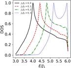
Finally, Figure 7 shows the density of states of the model. From this figure we observe that the density peaks undergo a shift to the right within the range $3\le \frac{E}{J_1}\le 6$ e.u. as we increase the influence of J₂. This results in a concentration in the population of excited magnons in higher energy bands, indicating the formation of an extra peak around $E/J_1=6$ e.u. at extreme values of $J_2=0.3J_1$.

4.2. Computational methods

This subsection is dedicated to discussing the computational methods used to obtain the graphs.We use the Python language for obtaining the graphs [³⁰] with the Matplotlib library [³¹]. The resolution of the graphs was set to 2000 × 2000 points, in order to deliver a good resolution in color maps without a large computational demand. The energy levels of the contour lines for the color map were set in the range of 2 to 6 e.u. (energy units) with 8 equally spaced divisions, totaling 9 contour lines, which is balanced enough to show the energy gradient without leaving the colormap overloaded with excessive contour lines. The colors used in the energy color map were generated with the "jet" color map, which is one of several colormaps avaliable in matplotlib library.

The three-dimensional graphs (Figure 3) were plotted in a similar manner, maintaining the same resolution (2000 × 2000) and the same energy range (2 to 6 e.u.). The two-dimensional projection of the 3D graph in the xy plane was positioned at $z=-2$, while the yz and xz projections were positioned at $x=-4$ and y = 4, respectively, in order to avoid obstruction of the projections (or part of them) by the three-dimensional surface.

The graphs of energy dispersion as a function of wave vector components and second neighbor interactions (Figure 4) were plotted with the same parameters used for the graphs in Figure 2, where the horizontal axis represents the x or y components of the wave vector, while the vertical axis represents the ratio of the intensity of interaction between the first and second neighbors.

The graph in Figure 5, which shows the energy value along a path connecting the high-symmetry points in the honeycomb lattice, was made by creating two lists of values for the x and y coordinates, respectively. The number of points in the lists was adjusted proportionally to the distance between the points at the ends of the segments delimited by two sites of high symmetry. Subsequently, the coordinates of each segment were concatenated into two lists to compose the x and y coordinates of the entire path. The graph in Figure 6 was generated by simply subtracting the curve for a given value of J₂ from a previous value, in other words, each curve corresponds to the variation that occurs in the energy under the effect of a change in the intensity of the interaction of second neighbors along the path connecting the high-symmetry points.

The distribution of the density of states for the energy values was created using a superposition of Lorentzian functions of the type

(25) $$DOS(E)=\frac{1}{\pi }\underset{\mathrm{\Gamma }\to 0}{\lim }{\displaystyle \sum _{i=1}^n{\displaystyle \sum _{j=1}^n\frac{{\mathrm{\Gamma }}^2}{{(E-E_{ij})}^2+{\mathrm{\Gamma }}^2}}},$$

where $\mathrm{\Gamma }$ is the Lorentzian band width, E_ij is the energy of a given point in the Brilouin zone (k-th pixel of the image), E is the energy value in the energy dispersion spectrum in the interval between the minimum and maximum values defined for the energy map graphs and n is the number of lines and collumns. For this graphs, $\mathrm{\Gamma }=0,25$ e.u., n=200 lines and wave vectors coordinates in the range of $-2\pi /a$ to $2\pi /a$, choice that avoids high computational costs and allows the visualization, without noise, of secondary peaks.

5. Conclusions

We investigated the free propagation of spin waves in a ferromagnet with honeycomb topology. It was observed that this topology does not favor the exchange interaction of second neighbors in the central region of the BZ, as happens with other geometries known in the literature, namely square and triangular. Another interesting aspect was the emergence of cone-like patterns of the dispersion relationship at points of high K symmetry, indicating that it is not a specific pattern for electronic analysis, but has its essence in the honeycomb topology itself. By adjusting the intensity J₂, we measure the coalescence effects in the BZ edge region, emphasizing the short-range character of the dominant exchange interactions in magnonic excitations with large wave vectors. As a direct result, we noticed the greatest energy variation at points M and K, the latter being more significant. Finally, we indicate the density of states (DOS) of the model, revealing the population of excited magnons in the spectral range $3\le E/J_1\le 6$ e.u. A sharp point is formed in the DOS pattern indicative of a Van Hove singularity, which moves to regions of higher energy due to the increase in J₂.

References

• ^[1] J.P. Jakubovics, Magnetism and magnetic materials (CRC Press, Boca Raton, 2023).
• ^[2] J.R. Sousa and C.A. Dartora, Revista Brasileira De Ensino De Física 43, e20210099 (2021).
• ^[3] A.P. Guimarães and I.S. Oliveira, Magnetismo e ressonância magnética em sólidos (Editora da Universidade de São Paulo, São Paulo, 2009)
• ^[4] F. Bloch, Zeitschrift Für Physik 61, 206 (1930).
• ^[5] H. Bethe, Zeitschrift Für Physik 71, 205 (1931).
• ^[6] T. Holstein and H. Primakoff, Physical Review 58, 1098 (1940).
• ^[7] J.H.E. Griffiths, Nature 158, 670 (1946).
• ^[8] C. Kittel, Physical Review 71, 270 (1947).
• ^[9] C. Herring and C. Kittel, Physical Review 81, 869 (1951).
• ^[10] F.J. Dyson, Physical Review 102, 1217 (1956).
• ^[11] C. Kittel, Physical Review 110, 1295 (1958).
• ^[12] P.A. Fleury, S.P.S. Porto, L.E. Cheesman and H.J. Guggenheim, Physical Review Letters 17, 84 (1966).
• ^[13] B. Hussain and M.G. Cottam, Journal of Physics: Condensed Matter 34, 445801 (2022).
• ^[14] R. Mondal and L. Rózsa, Physical Review B 106, 134422 (2022).
• ^[15] M. Golebiewski, R. Hertel, M. D'Aquino, V. Vasyuchka, M. Weiler, P. Pirro, M. Krawczyk, S. Fukami, H. Ohno and J. Llandro, ACS Applied Materials & Interfaces 16, 22177 (2024).
• ^[16] C. Ataca and S. Ciraci, Physical Review B 82, 165402 (2010).
• ^[17] K. Zberecki, Journal of Superconductivity and Novel Magnetism 25, 2533 (2012).
• ^[18] C. Gong, L. Li, Z. Li, H. Ji, A. Stern, Y. Xia, T. Cao, W. Bao, C. Wang, Y. Wang et al., Nature 546, 265 (2017).
• ^[19] W.F. Silva, C.G. Bezerra and R.N. Costa Filho, Solid State Communications 322, 114065 (2020).
• ^[20] T. Nakamura, Progress of Theoretical Physics 7, 539 (1952).
• ^[21] P.V.P. Madduri and S.N. Kaul, Journal of Magnetism and Magnetic Materials 418 143 (2016).
• ^[22] P.R. Wallace, Physical Review 71, 622 (1947).
• ^[23] K.S. Novoselov, A.K. Geim, S.V. Morozov, D. Jiang, Y. Zhang, S.V. Dubonos, I.V. Grigorieva and A.A. Firsov, Science 306, 666 (2004).
• ^[24] Y. Duan, C.D. Stinespring and B. Chorpening, ChemistryOpen 4, 642 (2015).
• ^[25] A.G. Vieira, R.M. Moraes, F.M. Vasconcelos and D.W. Maia, Revista Brasileira de Ensino de Física 45, e20230148 (2023)
• ^[26] F.R.V. Araújo, R.N.S. Magalhães, I.V. Sousa Jr., A.C.S. Nascimento and D.R. Costa, Revista Brasileira de Ensino de Física 44, e20220132 (2022).
• ^[27] I.N. Krivorotov, D.V. Berkov, N.L. Gorn, N.C. Emley, J.C. Sankey, D.C. Ralph and R.A. Buhrman, Physical Review B 76, 024418 (2007).
• ^[28] P.A. Grünberg, Reviews of Modern Physics 80, 1531 (2008).
• ^[29] M.S. Tavares, R.C.F. Pinto, E.V. Silva and A.V.N. Monroe, Solid State Communications 372, 115286 (2023).
• ^[30] Python, Python Docs, available in: https://www.python.org/doc/, accessed in: 07/09/2022.
  » https://www.python.org/doc/
• ^[31] J. Hunter, Computing in Science & Engineering 9, 90 (2007).

Publication Dates

• Publication in this collection
  07 Oct 2024
• Date of issue
  2024

History

• Received
  11 June 2024
• Reviewed
  07 Aug 2024
• Accepted
  30 Aug 2024