On approximate analytical solutions of transcendental equations

Abstract

In this paper, we provide a simple method to analytically solve general problems in science and engineering, which involve transcendetal functions. To validate the technique, we first compared our results to the exact solutions of two well-known problems, which are written in terms of transcendental equations: (1) circuit analysis of a resistor-diode association; (2) obtaining an analytical expression for the charge control in junctionless-nanowire FET devices. Next, to demonstrate the versatility of the method, we address the pendulum differential equation, to obtain an analytical expression for the period of the simple pendulum, considering any possible initial oscillation amplitude. None of these problems has a closed-form analytical solution. Alternatively, in all cases, simplified approximate analytical expressions were obtained, presenting low relative error when contrasted with the respective benchmark numerical results, thereby indicating that the approach can be considered quite accurate for most practical problems of interest.

Keywords
Transcendental equations; differential equations; analytical modeling; simple pendulum; nanoelectronic devices

1. Introduction

The need for analytical models in science and engineering has been intensified in the last few years because several large-scale practical problems do not allow the use computer-intensive numerical techniques. A typical example is integrated circuit design, which often involves the simultaneous simulation of several millions of transistors. The judicious approach is to employ low-complexity transistor models, simple enough to carry out this huge simulation task with a feasible computational effort. The trade-off is to assure that, albeit simplified, these models are still accurate enough to be a reliable tool in predicting the circuit performance.

It is the crucial to equip the students with tools to address these issues because, when building these analytical models, one often has to deal with mathematical problems involving transcendental functions, such as trigonometric, hyperbolic, exponential and logarithmic functions, and associated transcendental equations. In order to reach an analytical solution, it is usual to employ Taylor or Maclaurin series expansions of these elementary functions. However, such series expansions are only valid within strict range limits and often these limits do not fit a particular problem under study. In these cases, it is frequently necessary to use numerical routines to reach a satisfactory result. As an alternative, in this work, we provide a new development, which starts from the same Taylor series expansions but allow generalized solutions of transcendental equations. The method is simply called SAAMM (Simplified Approximate Analytical Mathematical Method) to translate the goal of obtaining simplified, yet accurate solutions for problems involving transcendental functions, while keeping the solutions fully analytical, without the need to resort to numerical techniques.

In a previous work, we briefly mentioned the use of SAAMM, when addressing the important technological issue of calculating the energy levels of finite quantum wells, a problem which does not have a closed-form analytical solution ^[1]. By applying the method ^[1], we obtained closed-form analytical expressions for every bound energy level, E_n, of finite quantum potential wells. Using the exact numerical solution as a reference, the model demonstrated quite good accuracy, and a very small relative error was achieved, of around 0.3%, for quantum well widths greater than 35 angstroms. These results indicate that our formulation is indeed a useful tool to help design nanoelectronic devices. The details of the method were to be provided elsewhere and are the focus of the present paper.

Thus here we detail the use of SAAMM. To exemplify and validate the technique, we compared our results to the exact solutions of two benchmark problems: (1) solving the transcendental equation arising from the analysis of a resistor-diode circuit association and (2) obtaining an analytical expression for the charge control in junctionless-nanowire FET devices. Next, to demonstrate the versatility of the method, we address the pendulum differential equation, to obtain an analytical expression for the period of the simple pendulum, considering any possible initial oscillation amplitude. None of these problems has a closed-form analytical solution. Alternatively, in our work simplified approximate analytical expressions were obtained. In all cases, when the analytical results are contrasted to the respective benchmark numerical solutions, the relative error indicates that the approach can be considered quite accurate for most practical problems of interest.

2. Simplified Approximate Analytical Mathematical Method

We call Simplified Approximate Analytical Mathematical Method (SAAMM) the technique in which we substitute the real variable,

(1) $$x=\theta +U,$$

in a real function, f(x), to alternatively write an approximate expression in terms of θ, the function f(θ). In Eq. (1), θ is a real variable, of very small value, and U is a real value defined by

(2) $$U=\frac{m}{j},$$

with j being a very large integer value, and

(3) $$m=\text{integer}\{jx\},$$

the closest integer value obtained from the product, jx.

3. Using SAAMM

SAAMM was originally conceived to solve polynomial and/or transcendental equations provided that an initial guess for the solution and the validity range of the approximations taken are properly established. In this work, we will systematically demonstrate the use of this tool to tackle equations of the type

(4) $$f(x)=0,$$

involving polynomial and/or transcendental terms and no exact analytical solution. To illustrate our procedure, one can conveniently split our approach into three steps. Next, we discuss each of the steps for implementing SAAMM.

3.1. First step

Goal: To determine the working range to find a rough initial guess, x₀, for the solution of interest. As usually happens in several techniques for solving transcendental equations, if needed, one can resort to a graphical method, aiming to determine the interval which contains the desired root, x_min ≤ x₀ ≤ x_max, called here the working range, from which we write

(5) $$x_0=(x_{\min }+x_{\max })/2,$$

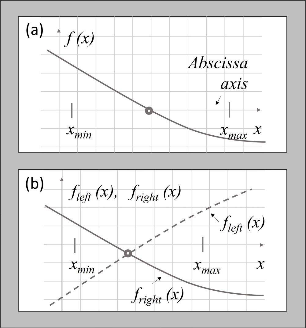
a crude approximation to the root of the equation to be solved, and the first step towards obtaining a more accurate result. To determine the working range, x_min and x_max can be selected on the basis of a graphical analysis. This graphical method allows for two distinct approaches for estimating the initial guess x₀. The first, illustrated in in Fig. (1-a), involves directly sketching the function f(x), and visually identifying its crossing point with the horizontal axis, corresponding to the root of the equation to be solved. Alternatively, the second approach, depicted in Fig. (1-b), leverages on the decomposition of f(x) into two functions, f_left(x) and f_right(x):

Figure 1
Schematic illustration of the graphical method: (a) function profile, f(x), and the search for an intersection point between the curve, f(x), with the x-axis, for an initial determination of an interval, x_min ≤ x₀ ≤ x_max; (b) function profile, f_left(x) e f_right(x), superimposed on the same scale, for an initial determination of an interval, x_min ≤ x₀ ≤ x_max, which contains a point of intersection between the curves, f_left(x) and f_right(x).

$$f(x)=f_{left}(x)-f_{right}(x)$$

Then, a sketch of the curves, f_left(x) and f_right(x), superimposed on the same axes, provides an initial estimate to the desired root of the equation, because the intersection point between them, where f_left(x) = f_right(x), corresponds to f(x) = 0, by the definition above. This decomposition offers additional freedom, allowing one to manipulate and analyze the components of f(x) separately, which can be advantageous when f(x) itself is complex or difficult to visualize directly. In either case, one can chose, almost arbitrarily, the values of x_min and x_max, provided that the Condition below is satisfied.

Condition 1The function, f(x), must be continuous and and preserve the sign of the derivative within the target interval, x_min ≤ x₀ ≤ x_max.

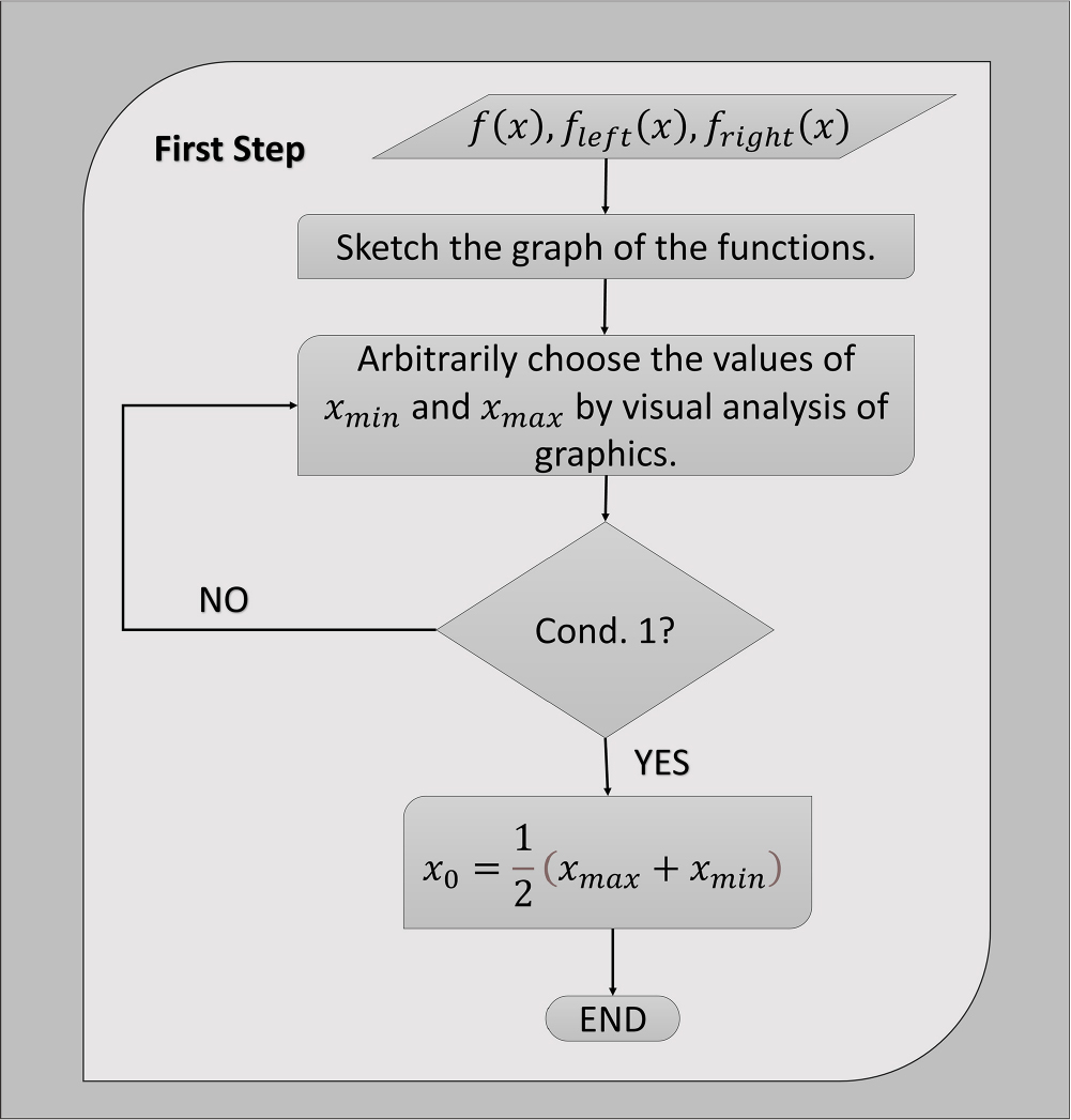
It is worth noting that, if the equation to be solved has more than one real roots, it is enough to find a working interval, x_mink ≤ x_0k ≤ x_maxk, for each of the k roots and repeat the procedure for each of them. Fig. (2), illustrates a summary of the processes involved in the first step of the method.

Figure 2
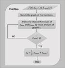
Summary of the processes composing the first step of this method, to obtain the initial guess, x₀.

3.2. Second step

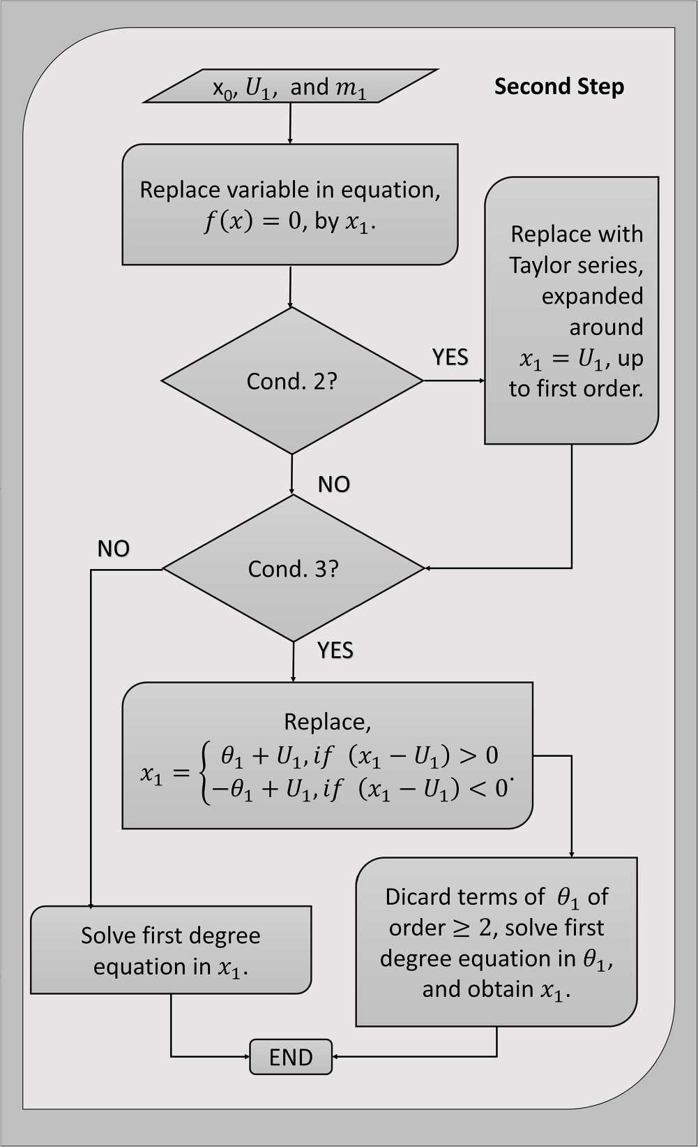
Goal: To determine a first approximation for the analytical root, x₁. For this, we proceed to solve, analytically, the equation f(x₁) = 0 (see Figure 3). If transcendental functions are present in the above equation, these functions should be replaced by the polynomial approximation resulting from its Taylor series expansion around the point x₁ = U₁. Usually, a first order expansion is enough (as it can be increased if desired) as long as the condition below is satisfied.

Figure 3
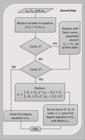
Flowchart of the sequence of operations involved in the third step of the method presented in this work for the analytical solution of polynomial or transcendental equations.

Condition 2 If the terms in x ₁ are only up to the first order, one has a first-degree equation, which can be easily solved to calculate x ₁ directly. On the other hand, if there are terms in x ₁ of order equal to or greater than two, we must replace x ₁ by

(6) $$x_1={\theta }_1+U_1,$$

resulting in an equation in terms of θ₁, in such way that f(θ₁) = 0, in which we must neglect all terms of θ₁ of order equal to or greater than two, to write a first-degree equation in θ₁. In doing so, we can obtain x₁ from θ₁, considering U₁ = m₁/j and m₁ = integer{jx₀}, with x₀, the initial guess, calculated in the first step, Eq. (5).

3.3. Third step

Goal: To determine an approximate analytical root of augmented precision, x₂. The third step consists of repeating the previous process, second step, and obtaining an approximate analytical solution of augmented precision,

$$x_2={\theta }_2+U_2,$$

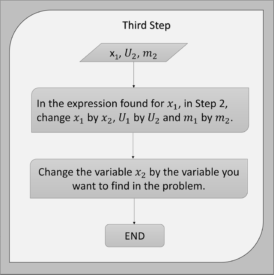
considering U₂ = m₂/j and m₂ = integer{jx₁}, with x₁ being the approximate value calculated in the second step, Eq. (6). Needless to say that the final result is the refined value for the variable x₂, which can be renamed as desired, considering the equation of interest. Fig. (4) depicts the flowchart describing the third step of the method.

Figure 4
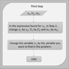
Flowchart of the sequence of operations involved in the third step of the method presented in this work for the analytical solution of polynomial or transcendental equations.

4. Some Additional Considerations

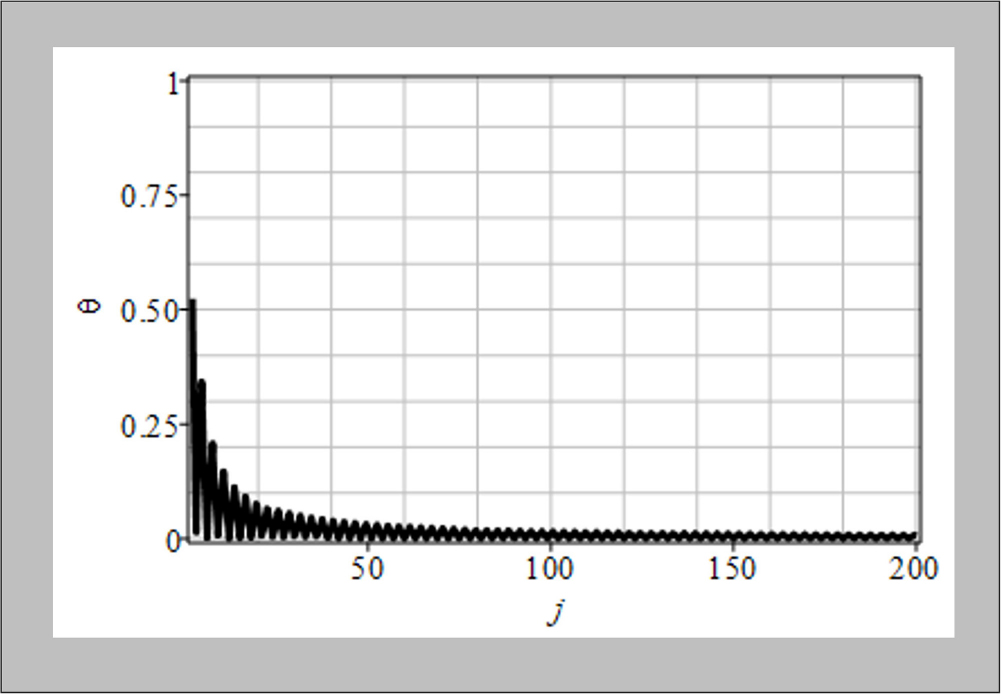
A feature of using SAAMM is that, the higher the value of j, the more accurate is the result obtained. This can be easily verified from a graphical analysis of the behavior of θ in function of j, when we consider, for instance, x = π/3, and

$$\theta =x-U,$$

in the graph of Fig. (5), because, as θ becomes progressively smaller, the value of j turns larger. This same behavior is expected whatever the value of x. Thus, our method, based on the Taylor series expansion of transcendental functions, becomes more and more precise, the smaller the value of θ, and therefore, the greater the value of j. A similar procedure should be performed for all roots of the equation, which are refered to by an index, k, to indicate to which interval the obtained result refers to. Finally, an analysis of the final result can be carried out to verify whether the results obtained reach the required degree of accuracy. If not, it is always possible to add more terms to the Taylor series expansion.

Figure 5
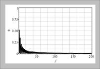
Graphical representation of the dependence of θ in terms of j, for x = π/3. The same behavior holds for any value of x.

5. Some Illustrative Applications

5.1. Current-voltage characteristics in a resistor-diode in-series association

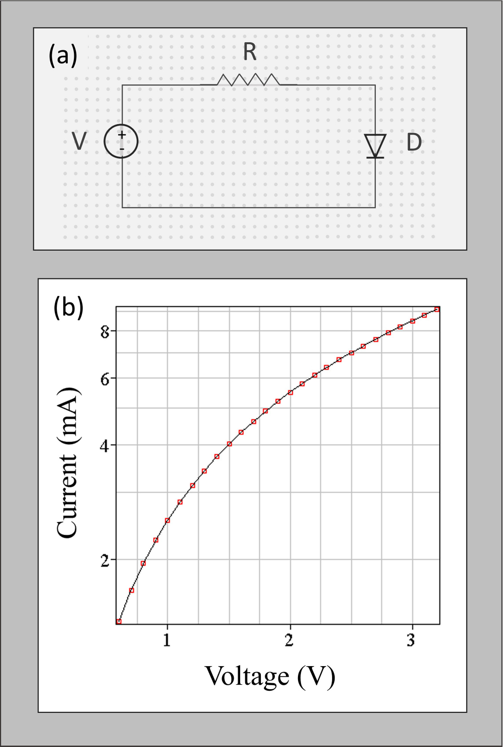
In this section we apply SAAMM to the problem of determining the current-voltage (I–V) relationship for the non-linear electronic circuit composed of an in-series association of a semiconductor diode, D, and a resistor, R, as depicted in Fig. (6-a). As well known, under a forward bias, the diode allows the current to flow, presenting only a small series resistance. On the other hand, under reverse bias, it prevents the current flow, allowing only a small reverse component I_s. The equation governing this specific resistor-diode series combination is given by:

Figure 6
(a) Resistor-diode in-series association. The following physical constants and circuit parameters were considered R = 330 Ω, I_s = 5 × 10⁻⁶ A, q = 1.602 × 10⁻¹⁹ C, T = 300 K, k_B = 1.38 × 10⁻²³ m²s⁻²kgK⁻¹. (b) Current-Voltage (I–V) relationship, provided by Eq. (14), by using SAAMM. The symbols represent the results provided by the analytical model, while the solid line represents the result obtained by using the platform Maplesoft.

(7) $$V-RI=\frac{k_{B}T}{q}\ln \left(\frac{I}{I_s}+1\right),$$

with, k_B, the Boltzmann constant, T, the absolute temperature, q, the elementary charge, and I_s, the saturation current. This simple relationship, very common in Electronics textbooks, does not have an exact analytical solution to express the current in terms of the bias voltage V , because Eq. (7) is a transcendental equation. Usually, to solve Eq. (7) and write the electric current as a function of the applied voltage, V , it is necessary to resort to numerical routines. However, by using SAAMM, this problem yields an interesting approximate analytical solution, which can be obtained on the basis of the flowcharts shown in Figs. (2)–(4), as it will be discussed below, in which we implement the three steps of the method. Note that Eq. (7) is written in such way that f_left(x) and f_right(x) are already naturally defined.

5.1.1. First step

The goal is to find the electric current variation as the bias voltage, V , sweeps the range 0.6 ≤ V ≤ 3.0 volts. The first step to apply the method is to determine the working interval I_min < I < I_max, and an initial guess, x₀., to extract the root, I, of the transcendental equation, Eq. (7) for each value of the applied voltage V. This task can be accomplished by inspection of a simple graphical sketch. Fig. (7) illustrates the technique used to find the working range from which we arbitrarily choose the interval defined by the current values, I_min = 10⁻¹² A < I < 5 × 10⁻² A = I_max. From these values of I_min and I_max, one can get the initial guess, starting from the Eq. (5), and writing

Figure 7
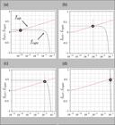
Technique used on the diode-resistor circuit problem, to find the current range, I, I_min < I < I_max, by means estimating approximate values of the root, I, while sweeping a voltage range from 0 < V < 3.0 volts. (a) 0.1 volts; (b) 0.3 volts; (c) 0.5 volts e (d) 3.0 volts.

(8) $$x_0=\frac{I_{min}+I_{max}}{2}$$

5.1.2. Second step

To maintain a uniform notation across the manuscript, the current variable, I, is changed to x₁, so that the equation to be solved is written as:

(9) $$V-R{x}_1=\frac{k_{B}T}{q}\ln \left(\frac{x_1}{I_s}+1\right).$$

As mentioned in the previous section, when the equation to be solved involves transcendental functions, one must first replace these terms with the polynomial approximations provided by the Taylor series expansion around the point, x₁ = U₁, until first order. In the case of Eq. (9), there is the logarithmic function, which needs to be approximated by its Taylor series expansion up to first order, around the point, x₁ = U₁, which results in:

(10) $$\ln \left(\frac{x_1}{I_s}+1\right)\approx \ln (F_1)+\frac{1}{I_s{F}_1}(x_1-U_1)$$

with F₁ = (U₁/I_s + 1). Replacing the polynomial approximation for the logarithm term into Eq. (9), the equation to be solved becomes:

(11) $$V-R{x}_1=\frac{k_{B}T}{q}[\ln (F_1)+\frac{1}{I_s{F}_1}(x_1-U_1)],$$

a first-degree equation, in x₁, which can be easily solved, taking U₁ = m₁j, m₁ = integer{jx₀}, with x₀ given by Eq. (8), where U₁ and m₁ are constants of the problem. Solving Eq. (11), one gets the following result for x₁:

(12) $$x_1=-\frac{(U_1+I_s)\left[c\mathrm{}\ln (F_1)-V\right]-c{U}_1}{R(U_1+I_s)+c}$$

with c = k_BT/q.

5.1.3. Third step

The third step consists of repeating the previous process, to obtain an approximate analytical solution of augmented precision, x₂, considering, U₂ = m₂j, m₂ = integer{jx₁}, with x₁ given by Eq. (12), the preliminary value of the analytical root, as calculated in the second step. In practice, this is equivalent to express the final result by an variable x₂, replacing x₁ by x₂, U₁ by U₂, and m₁ by m₂ in the previous step, so that we can write

(13) $$x_2=-\frac{(U_2+I_s)\left[c\mathrm{}\ln (F_2)-V\right]-c{U}_2}{R(U_2+I_s)+c}$$

with F₂ = (U₂/I_s + 1). Finally, by identifying the variable x, as the current I(V) we seek to calculate, one finds:

(14) $$I(V)=-\frac{(U_2+I_s)\left[c\mathrm{}\ln \left(F_2\right)-V\right]-c{U}_2}{R(U_2+I_s)+c}$$

Fig. (6-b) shows the I–V relationship, obtained from Eq. (14) by using SAAMM for the voltage range, 0.6 ≤ V ≤ 3.0 volts, in contrast to the numerical results provided by the Maplesoft software platform. The same computational tool was used to investigate the relative error concerning the approximate analytical results, which was below 0.0025%.

5.2. Cylindrical semiconductor nanowire as a voltage controlled gated-resistor

In this section, the SAAMM method is applied to a problem studied by us in ^[1], namely, the current-voltage (I–V) modeling of a cylindrical silicon semiconductor nanowire transistor of radius R₀. The device can be seen as a voltage-controlled resistor, often referred to as Junctionless Nanowire Field Effect Transistor – JLNWFET, widely considered a strong contender for the next generation of transistors. The devices of interest here have cylindrical symmetry and make use of three metallic contacts, two of them, the source and drain contacts, located at the ends of the semiconductor nanowire, while a third contact, involving the cylindrical surface of the nanowire, acts as a gate electrode.

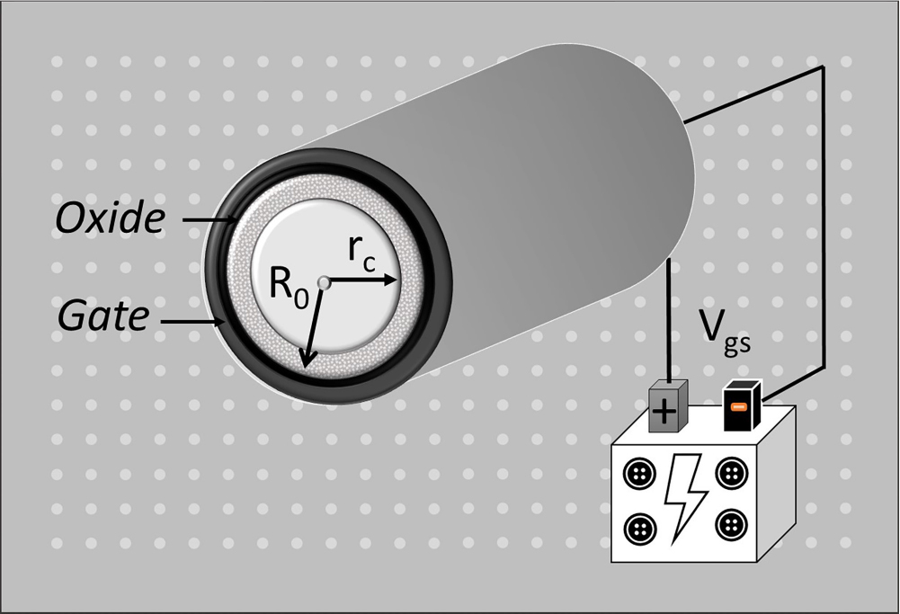
Also, as in any other MOS transistor, there is an oxide layer placed in between the gate contact and the semiconductor nanowire, as indicated in Fig. (8). The device is based on an active region of semiconductor material, with ionized doping density N_d uniformly distributed throughout the cylindrical, n-type semiconductor nanostructure, forming a conduction channel of radius r_c. Transistor action takes place because the channel radius and, consequently, the curret flow can be controlled when a gate-source voltage, V_gs, is applied to the gate contact. The electrostatic analysis of the device, by solving the Poisson equation, leads to a transcendental equation, Eq. (5) in [², ³], given by

Figure 8
Schematic representation of a cylindrical semiconductor nanowire resistor controlled by gate-source voltage, V_gs, showing the superficial gate electrode, an oxide layer, and the semiconductor nanowire, composed of two regions, as a function of the applied gate-source voltage: a depletion region, of thickness R₀ − r_c, and a conductive channel region, of radius, r_c.

(15) $$K_s\{R_0^2/2+r_c^2[\ln (r_c)-\ln (R_0)-1/2]\}=V_{gs}-V_{fb}+K_{ox}[R_0-r_c^2/R_0]$$

where ε_s and ε_ox are the dielectric permittivity for the semiconductor nanowire and oxide gate materials, respectively, w_ox is the oxide width, V_fb is the flat-band voltage, K_s = −qN_d/2ε_s and K_ox = qN_dw_ox/2ε_ox. The Eq. (15) is a transcendental equation expressing the so-called charge-control relation, which describes the radius of the conducting channel, the variable r_c, as a function of the gate voltage, V_gs, on the cylindrical semiconductor nanowire depicted in the Fig. (8). Knowledge of this relationship, r_c–V_gs, allows one to obtain both the current-voltage and the capacitance-voltage characteristics of the device. Applying SAAMM to this problem, by means of the three steps presented in the flowcharts shown in Figs. (2)–(4), yields an expression to relate the channel radius to the applied gate voltage, r_c(V_gs).

5.2.1. First step

As before, the first step is to determine the working interval and the initial guess, x₀. An analysis of the problem leads one to easily conclude that a consistent range for the channel radius, r_c, is to admit that the channel radius of the device can vary from r_{c min} = 0, up to a maximum value, corresponding to the physical radius of the nanowire, R₀. Then, r_{c max} = R₀ and 0 ≤ r_c ≤ R₀. From the values of r_{c min} and r_{c max}, we can write the initial guess, from the Eq. (5), as

(16) $$x_0=\frac{1}{2}(r_{c\max }+r_{c\min }).$$

5.2.2. Second step

In this step, to unify the notation used along the manuscript, we label the variable r_c as x₁, so that the equation to be solved is written as:

(17) $$K_s\{R_0^2/2+x_1^2[\ln (x_1)-\ln (R_0)-1/2]\}=V_{gs}-V_{fb}+K_{ox}[R_0-x_1^2/R_0].$$

As before, since there are terms of transcendental functions in the equation to be solved, it is necessary to first replace these terms with the polynomial approximations provided by the Taylor series, expanded around a point, x₁ = U₁, up to first order. In the case of Eq. (17), there is the logarithmic function, ln⁡(x₁), whose Taylor series expansion results in:

(18) $$\ln (x_1)\approx \log (U_1)+\frac{1}{U_1}(x_1-1).$$

Replacing this polynomial approximation into the logarithm term in Eq. (17), the equation to be solved becomes:

(19) $$K_s\{R_0^2/2+x_1^2[\log (U_1)+\frac{1}{U_1}(x_1-1)-\ln (R_0)-1/2]\}=V_{gs}-V_{fb}+K_{ox}[R_0-x_1^2/R_0],$$

a quadratic equation in x₁, with U₁ and m₁ being constants of the problem, given by U₁ = m₁/j, and m₁ = integer{jx₀}, with x₀ given by Eq. (16). Also, since the equation to be solved, f(x₁) = 0, is expressed as an equation with terms in x₁ equal to or greater than quadratic order, we must replace x₁, by, x₁ = θ₁ + U₁, and, in this new equation, neglect all terms of θ₁ of order equal to or greater than two. As a result, an approximate polynomial equation, of the first degree, in θ₁, is obtained. Finally, with the result for x₁, we can write, x₁ = θ₁ + U₁, which in this results in

(20) $$x_1=\frac{1}{A_1}\left(V_{gs}-B_1\right)+U_1$$

with

$$\begin{array}{l}{A}_1=\frac{2U_1}{R_0}\left[K_s\ln (U_1)R_0-K_s\ln (R_0)R_0+K_{ox}\right]\\ B_1=\frac{1}{2}{K}_s{R}_0^2+K_s{U}_1^2\ln (U_1)-K_s{U}_1^2\ln (R_0)+-\frac{1}{2}{K}_s{U}_1^2+V_{fb}-K_{ox}{R}_0+\frac{K_{ox}{U}_1^2}{R_0},\end{array}$$

constants of the considered problem.

5.2.3. Third step

The third step consists of repeating the previous process, to obtain an approximate analytical solution of augmented precision, x₂, considering U₂ = m₂/j, and m₂ = integer{jx₁}, with x₁ given by Eq. (20), the preliminary approximation for the analytical root, calculated in the second step. In practice, this is equivalent to express the final result by an variable x₂, recasting x₁ by x₂, U₁ by U₂, and m₁ by m₂ in the previous step, so that we can write

$$x_2=\frac{1}{A_2}\left(V_{gs}-B_2\right)+U_2\text{.}$$

Finally, we identify the variable x₂ as the variable to be calculated, in this case the conductor radius, r_c, to write

(21) $$r_c(V_{gs})=\frac{1}{A_2}\left(V_{gs}-B_2\right)+U_2,$$

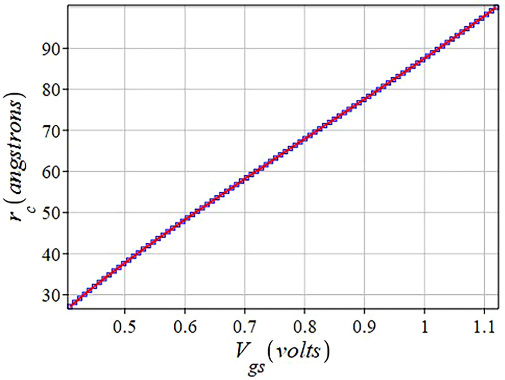
with A₁, A₂, B₁, B₂, U₁, U₂, m₁ and m₂, already described, as the constants of the problem solution. Fig. (9) show the plot r_c–V_gs, contrasting the analytical result obtained by Eq. (21), using SAAMM, with those provided by Maplesoft numerical platform. The relative error of the analytical results when compared to the Maplesoft solution is lower than 0.01%.

Figure 9
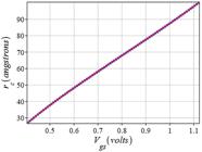
Conduction channel radius, r_c, as a function of the applied gate-source voltage, V_gs. For this problem the same values used in Ref. ^[1], were employed: a nanowire of radius R₀ = 100 Å, ionized donor doping concentration, N_d = 10¹⁹cm⁻³, and oxide layer thickness, w_ox = 20 Å. Also considered: k_d = 11.8, k_ox = 3.9, ε₀ = 8.85 × 10⁻¹²Fm⁻¹ e V_fb = 1.12 volts.

5.3. Finding the period of a simple pendulum

In this section, as yet another exemple of using SAAMM, to demonstrate the versatility of the method, we selected a different kind of problem. Specifically, we addressed the differential equation governing the problem of finding the period of a simple pendulum for the case of an arbitrary amplitude of the initial oscillation, α₀.

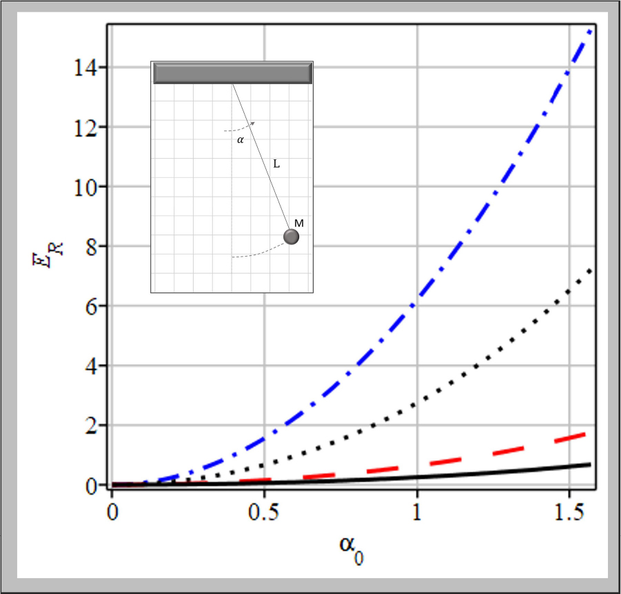
This simple pendulum is one of the most popular nonlinear systems covered in undergraduate and graduate textbooks, with numerous practical applications in physics and engineering because many natural phenomena are governed by a differential equation similar to the pendulum problem. Then, consider a simple pendulum like the one depicted in the top-left of Fig. (10), consisting of a body of mass, M, suspended by a long wire, of length L and of negligible mass, under the effect of the acceleration of gravity, g. In this system the body of mass M can be made to oscillate from an initial oscillation amplitude, α₀, which can be said to be in the range α_min < α₀ < α_max, with α_min = 0 and α_max = α₀. The differential equation representing the motion of a simple pendulum is then given by

Figure 10
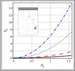
Comparison of the relative error for P₁, blue dot-dashed line (small oscillations model) and the relative error for P₂, black dot-line (SAAMM model, with original integration interval); red dashed line (SAAMM, integration using two segments); black solid line (SAAMM, integration using three segments). Top left: schematic representation of a simple pendulum, consisting of a body of mass, M, set to oscillate attached to a string of length, L, of negligible mass, under the effect of the acceleration of gravity, g. Parameters considered for this problem, L = 10 cm and g = 9.8 m/s². The benchmark to check the accuracy f the results takes the work by Nelson et al.^[12], as reference.

(22) $$\frac{d^2\alpha }{d{t}^2}=-\frac{g}{L}\sin \alpha ,$$

in which α is the angle of oscillation of the pendulum at a given time t. The initial conditions the problem are written as:

$$\alpha (t=0)={\alpha }_0\text{and}\frac{d\alpha }{dt}{|}_{t=0}=0.$$

The differential equation given by Eq. (22) does not have a straightforward solution, because of the term sin⁡(α). Only in particular cases, where small angles of oscillations are considered, it is possible to simplify the solution by taking sin⁡(α) ≈ α. In this case, the differential equation describing the pendulum motion can be approximated by the more familar linear differential equation, much easier to solve:

(23) $$\frac{d^2\alpha }{d{t}^2}=-\frac{g}{L}\alpha .$$

Eq. (23) yields an exact analytical solution in terms of elementary functions, α (t) = α₀ cos ⁡(ω₀t), with α₀≪1 and the motion angular frequency given by ${\omega }_0=\sqrt{g/L}$. From the angular frequency, one can write the period of oscillation in the case of small angles as P₀, related to the angular frequency by ω₀ = 2π/P₀, in such way that:

(24) $$P_0=2\pi \sqrt{L/g}.$$

But, as this result can only be used for small oscillation angles, to cover the entire range of possible initial oscillations, 0 < α₀ < π/2, another strategy is necessary. In fact, there are several studies in the literature on this topic [⁴, ⁵, ⁶, ⁷, ⁸, ⁹, ¹⁰, ¹¹]. In particular, Nelson et al.^[12] obtained an exact analytical solution for the problem, considering any initial value for α₀. They solved the full differential equation, describing the motion of the pendulum, in terms of elliptic Jacobi functions, in such way that the period of the pendulum oscillation can be written as:

(25) $$P_1=P_0{{\displaystyle \sum _{n=1}^{\infty }\left(\frac{(2n)!}{2^{2n}{(n!)}^2}\right)}}^2{\sin }^{2n}(\frac{{\alpha }_0}{2}).$$

This exact expression will be used as a benchmark for comparison against our analytical results.

Although the solution proposed by Nelson et al.^[12] is certainly fully analytical, it is not easy to handle and that is why in the literature one finds a variety of simplification schemes for this problem. Considering the relevance of the problem ^[13], we proceed to apply SAAMM to solve Eq. (22), thereby showing that we can obtain an approximate yet quite accurate analytical result. In what follows, we will demonstrate how to use SAAMM to find the period of the simple pendulum, for any initial oscillation amplitude, α₀. To do so, we employ an usual integration strategy, carrying out the change of variables u = dα/dt, so that Eq. (22) becomes

(26) $$\frac{du}{dt}=-\frac{g}{L}\sin \alpha .$$

Integrating Eq.(26), one obtains,

(27) $$u=\sqrt{\frac{2g}{L}\left[\cos (\alpha )-\cos \left({\alpha }_0\right)\right]}.$$

which, in turn, can be integrated again, keeping in mind that u = dα/dt, to arrive at the following result:

(28) $$\frac{d\alpha }{\sqrt{\frac{2g}{L}\left[\cos (\alpha )-\cos ({\alpha }_0)\right]}}=dt.$$

At this point we can apply SAAMM to find the period of the pendulum, which we will refer to as P₂. To find P₂ it suffices to consider a convenient integration interval in Eq. (28), more precisely a quarter of the period, P₂/4, which results in

(29) $$P_2=4\sqrt{\frac{L}{2g}}{\displaystyle {\int }_0^{\alpha 0}\frac{d\alpha }{\sqrt{[\cos (\alpha )-\cos ({\alpha }_0)]}}}.$$

The term, cos⁡(α) in Eq. (29), can be replaced by the approximate quadratic function, fcos, found in Eq. (B.1). For the algebraic manipulations to follow, consider the representation below:

(30) $$(\mathrm{\dots })=\frac{1}{\sqrt{\left[fcos-\cos ({\alpha }_0)\right]}}.$$

Using the representation shown in Eq. (30), the Eq. (29) can be written approximately as

(31) $$P_2=4\sqrt{\frac{L}{2g}}{\displaystyle {\int }_0^{\alpha 0}(\text{…})d\alpha .}$$

Knowing the result of the integral,

$${\displaystyle \int \frac{d\alpha }{\sqrt{[-a{\alpha }^2-b\alpha +d]}}=\frac{1}{\sqrt{a}}\arctan (\frac{\sqrt{a}(\alpha +\frac{b}{2a})}{\sqrt{-a{\alpha }^2-b\alpha +d}})=K(\alpha ),}$$

one can write an approximate analytic expression for the period of the pendulum, as

(32) $$P_2=4\sqrt{\frac{L}{2g}}\left[\frac{\pi }{2\sqrt{a}}-K\left({\alpha }_{\min }\right)\right],$$

with m = integer{j (α_min + α_max)/2}, S = cos⁡(U), T = sin⁡(U), U = m/j, a = S/2, b = T−SU, c = S−SU²/2 + TU and d = c−cos⁡(α₀). Taking the work of Nelson et al.^[12] as a benchmark for the value of the exact period, P₁, it is seen that, by inspection of Fig. (10), our approximate analytical result for the period, P₂, represented by the dot curve arising from the above equation, is more accurate than the usual small-oscillation framework, represented by the dot-dashed curve. Specifically, the conventional small-oscillation approximation results in a relative error that can reach up to 15.27%. In contrast, our initial approximation provides improved accuracy, yielding a relative error of, at most, 7.21%. Since this accuracy may be not enough for some applications, we carried out an additional step, by realizing that the integral in Eq. (31) can be conveniently split, since the approximate function of the cosine, fcos, Eq. (B.1), can be written as a piecewise function as follows

$$Fco{s}_l(\alpha )=\{\begin{array}{c}\hfill fco{s}_1(\alpha ),{\alpha }_1\le \alpha \le {\alpha }_2,\hfill \\ \hfill \mathrm{\dots }\hfill \\ \hfill fco{s}_i(\alpha ),{\alpha }_i\le \alpha \le {\alpha }_{i+1},\hfill \\ \hfill \mathrm{\dots }\hfill \\ \hfill fco{s}_l(\alpha ),{\alpha }_i\le \alpha \le {\alpha }_{l+1},\hfill \end{array}$$

with

$$fco{s}_i(\alpha )=-a_i^2{\alpha }^2-b_i\alpha +c_i,$$

in which i is an integer used as an index i = 1, 2, 3, …, l, while l represents the number of segments of an interval, and the number of subintervals of this interval: α_i = α₁ + (i−1)α₀/l. In this particular case, α₁ = α_min and α_{l + 1} = α_max. The parameters of the SAAMM method can be obtained as before, considering U_i,l = m_i,l/j and m_i,l = integer{jx_0i}, and the initial guess, x_0i, for each interval or subinterval, given by:

$$x_{0i}=\frac{(2i-1){\alpha }_0}{2l}.$$

For the case where the interval is split in two, then, l = 2, one can write:

$$Fco{s}_2(\alpha )=\{\begin{array}{c}\hfill -a_1^2{\alpha }^2-b_1\alpha +c_1,0\le \alpha \le {\alpha }_0/2,\hfill \\ \hfill -a_2^2{\alpha }^2-b_2\alpha +c_2,{\alpha }_0/2\le \alpha \le {\alpha }_0\hfill \end{array}$$

From this, it is possible to rewrite the integral as Eq. (31), in such way that

$${\displaystyle {\int }_0^{\alpha 0}\left(\cdots \right)}d\alpha ={\displaystyle {\int }_0^{\alpha 0/2}(\cdots )}1d\alpha +{\displaystyle {\int }_{\alpha 0/2}^{\alpha 0}(\cdots )}1d\alpha$$

with

$${(\mathrm{\dots })}_1=\frac{1}{\sqrt{\left[fco{s}_1-\cos ({\alpha }_0)\right]}},$$

$${(\mathrm{\dots })}_2=\frac{1}{\sqrt{\left[fco{s}_2-\cos ({\alpha }_0)\right]}}.$$

In this case, the period results as

$$P_2=4\sqrt{{\displaystyle \frac{L}{2g}}}[{\displaystyle \frac{\pi }{2\sqrt{a_2}}}+K_1\left({\displaystyle \frac{{\alpha }_{\max }}{2}}\right)+-K_1\left({\alpha }_{\min }\right)-K_2\left({\displaystyle \frac{{\alpha }_{\max }}{2}}\right)],$$

and the relative error drops significantly, as it can be seen in the dashed line curve in the Fig. (10), which reaches a maximum of 1.74%. Also, if the integration interval is split into three segments, the relative error does not exceed 0.68%, as it can be seen by the solid line curve, in Fig. (10). In this way, the technique allows increased accuracy for the analytical results if the number of segments is also increased.

6. Conclusions

The Simplified Approximate Analytical Method (SAAMM) introduced in this work was successfully demonstrated in several tasks, including to write approximations for transcendental functions, as well as to solve polynomial and/or transcendental equations in problems which, in principle, do not allow an analytical solution. To exemplify the use of the method, we discussed some important applications. Specifically, we applied SAAMM to a few canonical problems in electronic circuits analysis, nanoelectronics devices and fundamental physics.

From the basic electronics point of view, the first problem was to determine the current-voltage relationship, I–V, of a non-linear electronic circuit combination, composed of a semiconductor diode and a resistor, a problem which does not have a closed-form solution. Next. the second problem addressed was the application of SAAMM to the modeling of cylindrical junctionless semiconductor nanowire transistors (JL-NW-FETs), widely regarded as possible candidates for a future generation of transistors. Specifically, we provided approximate analytical expression for the radius of the conduction channel within the nanowire as a function of the applied gate voltage. When compared to the results provided by numerical tools, such as the Maplesoft platform, we achieved very low relative errors, showing that this methodology can be useful to determine the current-voltage and capacitance-voltage characteristics of these devices, which are relationships of fundamental importance for nanoelectronics.

From a basic physics point of view, SAAMM was also very successfully applied to the approximate solution of the differential equation governing the period of the simple pendulum, encompassing the case of any arbitrary initial oscillation amplitude. The proposed method provided a more accurate result than the one obtained by using the small oscillations model, which can yield a relative error of 15.27%, when α₀ = π/2, against the 7.21% provided by SAAMM. In addition, for the cases in which this relative error may still be considered too high, an additional strategy was used to provide greater accuracy to the results. The strategy was to write the simplified approximate cosine function as a convenient piecewise function. By adopting this strategy, it was found that the relative error drops significantly, to well below 2%.

In conclusion, the proposed method, SAAMM, offers significant computational advantages over traditional iterative numerical methods, such as the Newton-Raphson method. While iterative methods require multiple evaluations of the function and its derivative at each iteration, SAAMM obtains an approximate solution analytically, drastically reducing the need for numerical evaluations. This characteristic results in a smaller number of arithmetic operations and, consequently, lower computational cost, especially in problems with complex functions or that require high precision. Furthermore, the analytical nature of the solution obtained with SAAMM facilitates the sensitivity analysis of the solution with respect to the problem parameters, a task that can be computationally expensive in iterative numerical methods. In the Appendix we provide a series of useful steps and relationships, to solve several kinds of polynomial and transcendental equations.

Appendix

A. Solving Polynomial Equations

As it is well known, the solution of polynomial equations becomes increasingly difficult as the degree, n, of the polynomial equation grows. SAAMM is a very useful tool for obtaining simplified approximate analytical solutions for different types of problems, particularly for solving polynomial functions of the type,

(A.1) $$a_n{x}^n+a_{n-1}{x}^{n-1}+\mathrm{\dots }+a_i{x}^i+\mathrm{\dots }=0,$$

in which, a_i is the real coefficient pertaining the term xⁱ, with x a real variable and i and n interger numbers. To find the simplified approximate analytic roots of polynomial equations, it is enough to follow the three steps presented in the flowcharts of Figs. (2)–(4), as it will be discussed below.

A.1. First step

Make a preliminary graphical sketch of how many roots there are within the working interval, x_min ≤ x₀ ≤ x_max. Next, provide the initial guess, x₀, and verify the continuity of the function, f(x), within the selected interval, making sure that the sign of the derivative is unchanged within the interval. In this way, for each considered interval, the equation root exists and it is unique.

A.2. Second step

Recast the variable of interest for the problem as x₁, and write f(x₁) = 0. For the polynomial equation of degree, n, equal to or greater than two, replace x₁ by Eq. (6), in order to obtain an equation, in θ₁, given by:

(A.2) $${\alpha }_n{({\theta }_1+U_1)}^n+{\alpha }_{n-1}{({\theta }_1+U_1)}^{n-1}+\cdots +{\alpha }_i{({\theta }_1+U_1)}^i+\cdots +{\alpha }_1{({\theta }_1+U_1)}^n+{\alpha }_0=0$$

From the Eq. (A.2), and carrying out all the required mathematical operations, one arrives at an equation in θ₁, written as:

$$a^n{\theta }_1+\mathrm{\cdots }+a_i{\theta }_1^i+\mathrm{\cdots }=0,$$

In SAAMM, as j grows, θ₁ becomes progressively smaller, as it can be seen in the Fig. (5). Thus, by taking j as a very large value in our approximation, it is possible to neglect all terms of θ₁ of power equal to or greater than two, in order to obtain a simplified equation, of the first degree for θ₁, and finally write x₁ = θ₁ + U₁, for each of the considered intervals.

A.3. Third step

The third step consists of repeating the previous process, and obtaining an approximate analytical solution of augmented precision, x₂ = θ₂ + U₂, considering U₂ = m₂/j and m₂ = integer{jx₁}, with x₁, the approximate analytical root, calculated in the second step, Eq. (6). In practice, this is equivalent to recasting the previous result for x₁, taking x₁ as x₂, U₁ as U₂ and m₁ as m₂. The same procedure must be carried out for each working interval which contains a root of the equation.

B. Approximation for Transcendental Functions

In many scientific problems, the presence of some elementary functions in an equation, such as, sin(x), sinh(x), log(x), exp(x), etc., may prevent an analytical solution.Within the SAAMM framework, we provide approximate expressions for the various functions which may appear in transcendental equations.

B.1. Trigonometric functions

One can write an approximate function, fsinx, for the function sin⁡(x), using the polynomial terms given by the Taylor series of this function, expanded around x = U, up to a desired order, for example, first order, resulting in

$$fsinx=Sx+(T-SU),$$

with S = cos⁡(U), T = sin⁡(U). Similarly, using this procedure, we can obtain an approximate function for any trigonometric function. Following this same reasoning, the approximate function for the cosine results,

$$fcos=-Tx+(S+TU).$$

If greater precision is needed, more terms can be added to the Taylor series to further increase the accuracy of the results. For example, if additional terms are considered in the Taylor series expansion of the function cos⁡(x), a parabolic approximation, fcos, results in:

(B.1) $$fcos=-a{x}^2-bx+c$$

with a = S/2, b = T − SU, and c = S − SU²/2 + TU.

B.2. Hyperbolic functions

A similar procedure can be used to obtain approximate functions for the hyperbolic functions as well. Following this same script, the approximate functions for sinh⁡(x) and cosh⁡(x), result in

(B.2) $$\begin{array}{c}\hfill fsinh=Px+(R-PU)\hfill \\ \hfill fcosh=Rx+(P-RU)\hfill \end{array}\}$$

with R = sinh⁡(U) and P = cosh⁡(U).

B.3. Exponential functions

In the same way, one can express an approximation for the exponential function, e^x:

(B.3) $$fexp=e^U(x+1-U)$$

B.4. Logarithm functions

This method of simplification can also be used for the logarithmic function, to write

(B.4) $$flogx=\log (U)+\frac{1}{U}\left(x-1\right)$$

Data Availability

Simulation data can be made available upon request directly to the authors.

References

• ^[1] D.R. Celino, R. Ragi and M.A. Romero, J. Comput. Electron. 20, 2411 (2021).
• ^[2] R. Ragi, R.T. Nobrega, U.R. Duarte and M.A. Romero, IEEE Trans. Nanotechnol. 15, 627 (2016).
• ^[3] R. Ragi and M.A. Romero, IEEE Trans. Nanotechnol. 18, 762 (2019).
• ^[4] F.M.S. Lima and P. Arun, Am. J. Phys. 74, 892 (2006).
• ^[5] A. Beléndez, C. Pascual, D.I. Méndez, T. Beléndez and C. Neipp, Rev. Bras. Ens. Fis. 29, 645 (2007).
• ^[6] A. Beléndez, J. Francés, M. Ortuño, S. Gallego and J.G. Bernabeu, Eur. J. Phys. 31, L65 (2010).
• ^[7] M.I. Qureshi and K.A. Quraishi, Gen. Math. Notes 3, 50 (2011).
• ^[8] A. Beléndez, E. Arribas, A. Márquez, M. Ortuño and S. Gallego, Eur. J. Phys. 32, 1303 (2011).
• ^[9] J.P.J. Neto, Int. J. Appl. Math. 30, 259 (2017).
• ^[10] F.M.S. Lima, Rev. Bras. Ens. Fis. 41, e20180202 (2019).
• ^[11] S.S. Abdulkareem, A. Akgül, V.J. Jalal, B.M. Faraj and O.G. Abdulla, Therm. Sci. 24, S25 (2020).
• ^[12] R.A. Nelson and M.G. Olsson, Am. J. Phys. 54, 112 (1986).
• ^[13] T. Bensky, Longitude, Time, and Navigation (Independently published, 2018), 2 ed.

Edited by

• Editor-in-Chief:
  Marcello Ferreira https://orcid.org/0000-0003-4945-3169

Publication Dates

• Publication in this collection
  20 June 2025
• Date of issue
  2025

History

• Received
  07 Sept 2024
• Reviewed
  27 Mar 2025
• Accepted
  07 May 2025