Magnetotelluric method: theoretical deduction, analytical solutions and numerical modeling in a one-dimensional Earth
Abstract
The magnetotelluric (MT) method is a passive geophysical technique that uses natural variations in electromagnetic fields to investigate the Earth’s subsurface resistivity structure. This article has a didactic objective: to guide students of physics and geophysics, at any level, through the theoretical foundations and mathematical derivations underlying the 1D MT method. Starting from Maxwell’s curl equations in the frequency domain, we derive wave-like differential equations for the electric and magnetic field components in a conductive medium. These equations lead to analytical solutions that describe the attenuation and phase shift of electromagnetic waves as they propagate through layered Earth models. From these results, we deduce expressions for the MT impedance and phase. The step-by-step presentation is complemented by simple computational implementations in Python for 1D models, enabling readers to connect the theoretical concepts with practical applications. By presenting the methodology in a clear and structured way, this work aims to support students and educators in developing a deeper understanding of the magnetotelluric method and its role in subsurface exploration.
Keywords:
Geophysics; Geophysical Method; Magnetotelluric Method; Maxwell Equations; Forward Modeling
Resumo
O método magnetotelúrico (MT) é uma técnica geofísica passiva que utiliza variações naturais em campos eletromagnéticos para investigar a estrutura de resistividade do subsolo da Terra. Este artigo tem um objetivo didático: guiar estudantes de física e geofísica, em qualquer nível, através dos fundamentos teóricos e derivações matemáticas que fundamentam o método de MT unidimensional. Partindo das equações rotacionais de Maxwell no domínio da frequência, derivamos equações diferenciais ondulatórias para as componentes dos campos elétrico e magnético em um meio condutor. Essas equações levam a soluções analíticas que descrevem a atenuação e o deslocamento de fase das ondas eletromagnéticas à medida que se propagam através de modelos terrestres em camadas. A partir desses resultados, deduzimos expressões para a impedância e a fase da MT. A apresentação passo a passo é complementada por implementações computacionais simples em Python para modelos unidimensionais, permitindo que os leitores conectem os conceitos teóricos com aplicações práticas. Ao apresentar a metodologia de forma clara e estruturada, este trabalho visa apoiar estudantes e educadores no desenvolvimento de uma compreensão mais aprofundada do método magnetotelúrico e seu papel na exploração do subsolo.
Palavras-chave:
Geofísica; Método Geofísico; Método Magnetotelúrico; Equações de Maxwell; Modelagem Direta
1. Introduction
Geophysics is an applied science that investigates subsurface structures by analyzing the physical properties of rocks, using a variety of instrumental techniques known as geophysical methods. These methods are classified according to the main physical property they measure, such as potential field methods (e.g., gravity and magnetics), seismic methods, and electromagnetic methods. The magnetotelluric (MT) method is part of a group of electromagnetic techniques that measure natural variations in the Earth’s electromagnetic fields.
The MT method was independently introduced by Tikhonov [1] and Cagniard [2]. It is based on the simultaneous measurement of the horizontal components of the natural electric and magnetic field variations at the Earth’s surface to infer the subsurface geoelectric structure. Initially developed for one-dimensional models, where electrical resistivity varies solely with depth-the method has since undergone significant advancements, enabling its application to more complex two- and three-dimensional geological settings.
Although the MT problem is well established and has been extensively studied, this paper consolidates prior knowledge by presenting three different approaches to its resolution for 1D case. This paper provides a concise overview of the theoretical foundations and governing equations of the MT method. It also includes the derivation of analytical expressions for electromagnetic wave diffusion, leading to the formulation of apparent resistivity and phase equations. In addition, compute modeling equations are provides through simplified Python codes, based on theoretical formulations. All codes are made available for download, aiming to support students and researchers in understanding and applying the MT method.
2. Magnetotelluric Method
The MT method provides subsurface imaging with an intermediate resolution between reflection seismic and potential field methods [3]. Among geophysical techniques, MT stands out for its exceptional investigation depth, capable of probing from tens of meters to several hundred kilometers [4].
Eletromagnetic methods enable resource prospecting by measuring the effects of eletric current flowing in the surface. The MT method depends on naturally occurring varying electromagnetic fields present at the Earth’s surface. Understanding the sources of these electromagnetic signals is fundamental to interpreting MT data as they determine the frequency range and, consequently, the depth of investigation.
Electromagnetic signals used in MT span a wide range of frequencies, each associated with different physical processes as illustrated on Figure 1. High-frequency signals () are generated in the region between the Earth’s surface and the ionosphere, primarily due to lightning discharges, electromagnetic phenomena commonly referred to as sferics. These signals dominate the audio-frequency range and are useful for shallow investigations.
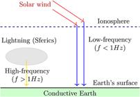
In contrast, low-frequency signals () originate from the interaction between charged particles in the solar wind and the Earth’s magnetosphere and ionosphere, producing ultra-low frequency (ULF) variations that enable deep subsurface exploration.
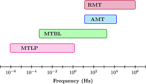
A key aspect of MT is that it allows geophysicists to investigate multiple death layers by analyzing signals in different frequency bands. The ability of electromagnetic waves to penetrate the Earth depends on their frequency: lower frequencies reach deeper regions, while higher frequencies are limited to near-surface layers. This phenomenon is described by the concept of skin depth, which will be explored in the next sections. Consequently, the MT method is commonly subdivided into four principal frequency bands, Figure 2, each associated with specific signal sources and depth ranges.
Each frequency band is selected depending on the target depth and geological context. Modern MT surveys often combine measurements from multiple bands to construct a comprehensive image of the subsurface across several depth scales.
Long-Period MT (MTLP): Covers ultra-low frequencies typically below 1 Hz, down to . These signals originate from global-scale interactions between the solar wind and the Earth’s magnetosphere and ionosphere. MTLP is particularly suited for crustal studies capturing both shallow and intermediate-depth structure.
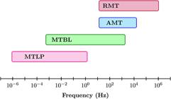
Subdivisions of the magnetotelluric method according to frequency range: MTLP (long-period), MTBL (broadband), AMT (audio), and RMT (radio).
Broadband MT (MTBL): spanning approximately from to , broadband MT is the most widely used range in crustal studies. Capturing both shallow and intermediate-depth structures.
Audio-Magnetotellurics (AMT): Operating in the range of roughly to , AMT is dominated by high-frequency electromagnetic signals caused by lightning discharges (sferics). This band is well-suited for resolving shallow subsurface features, such as sedimentary basins, aquifers, or near-surface faults.
Radio-Magnetotellurics (RMT): Extending from approximately to , RMT uses man-made radio transmitters as the main source of signal. It provides high-resolution imaging of very shallow structures, typically within the first tens of meters below the surface.
Although RMT operates in the frequency range from approximately to , using man-made radio transmitters as the primary source of signal, this article focuses specifically on natural-source methods, such as those driven by ionospheric and magnetospheric variations.
Unlike other MT subdivisions, which relies on naturally occurring electromagnetic fields, RMT introduces controlled artificial sources, which may require distinct mathematical formulations, especially in terms of boundary conditions and far-field approximations.
Similarly, methods like Controlled-Source Audio Magnetotellurics (CSAMT) also fall outside the scope of this work, as they depend on transmitter-receiver setups with designed signal characteristics. These techniques are valuable for high-resolution imaging of shallow subsurface layers, but their reliance on non-natural sources introduces different theoretical assumptions.
For these reasons, RMT and CSAMT are not addressed here, and the theoretical developments, derivations, and modeling presented in this article are exclusively based on the natural-source MT method.
2.1. Boundary conditions
Nabighian [5] affirms that the resultant field of electromagnetic problems is the sum of the primary and secondary fields. Each of the fields must satisfy Maxwell’s equations, or equations derived therefrom, plus appropriate conditions to be applied at boundaries between the homogeneous regions involved in the problem, e.g., at the air–earth interface.
Boundary conditions can be divided into two main categories: those derived from the normal components and those from the tangential components of the electromagnetic fields. Each category leads to specific constraints on the behavior of the fields , , , , and , as well as on the scalar potentials and , and the vector potentials and . The main boundary conditions are summarized schematically in Figure 3. For detailed information, check Griffiths [6] section 7.3.6.

2.2. Normal
The normal component of the magnetic field does not present discontinuity when passing from one medium to another. This is due to the absence of magnetic monopoles and follows directly from Maxwell’s equation (7).
2.3. Normal
The normal component of the electric displacement field is generally discontinuous across an interface due to the accumulation of surface charge density . This condition is expressed as as presented on Figure 4.

In MT method, it is common to assume the absence of free surface charge at the interfaces between geological layers, leading to the simplified boundary condition. However, this condition becomes particularly relevant in the presence of dielectric interfaces, such as the transition between air and soil, or between rock and a fluid with different electrical conductivity. In such cases, discontinuities in the normal component of the electric displacement field may arise due to surface charge accumulation.
2.4. Tangencial
The tangential condition for the electric field is expressed as . That is, the tangential electric field is continuous across an interface, provided there is no abrupt variation in potential or surface current sources.
2.5. Tangencial
The tangential condition for the magnetic field is given by , this means that the tangential component of the magnetic field is continuous across an interface, as long as there is no surface current density present.
In geophysical practice, particularly in the MT method, it is commonly assumed that the magnetic permeability is equal to that of free space, i.e., , since most geological materials are not strongly magnetic. This leads to and . Thus, in MT modeling, this boundary condition is often simplified to continuous.
However, this simplification may not hold in cases involving materials with significant magnetization, such as iron-rich rocks or models with strong contrasts in magnetic permeability .
2.6. Current density
The boundary condition for the current density vector is expressed as . That is, the normal component of the current density is continuous across an interface. Strictly speaking, this result is valid for direct currents. However, it is generally acceptable for Earth materials up to frequencies of approximately Hz where the displacement current can be neglected [5],
2.7. Scalar potentials
For static fields, the eletrical scalar potential and magnetic one can be matematically described by,
The scalar electric potential and the scalar magnetic potential must be continuous across an interface. This ensures that the work done in moving a small test charge or magnetic dipole across the boundary is path independent, where and .
In geophysical applications, this condition is relevant in low-frequency or static approximations, where fields are derived from scalar potentials rather than from time-varying vector fields.
2.8. Vector potentials
The Schekkunoff vector potentials are more complex consideration of fields that facilitate the boundary condition applications by separating the variables of the system in symmetry problems. There are two types of vector potentials: the magnetic and electric.
Chart 1 Types of sources for Schelkunoff vector potentials.| Magnetic Vector Potential | Electric Vector Potential |
|---|---|
|
Magnetic dipole perpendicular to a layered Earth Infinite cylinder in a uniform inducing magnetic field |
Electric dipole perpendicular to a layered Earth Cylinder in a uniform electric field |
|
Sphere in a uniform inducing magnetic field Horizontal magnetic dipole |
Sphere in a uniform electric field Horizontal electric dipole over a layered Earth |
Dipoles perpendicular to a layered Earth allow vertical stratification and 1D modeling; The cylindrical and spherical geometries are used to derive analytical solutions in 2D and 3D cases, serving as benchmarks for validating numerical codes. Also the horizontal dipoles better represent field conditions in near-surface geophysics, such as in magnetotelluric or controlled-source EM methods.
Understanding the physical origin of each potential and its associated source helps clarify why different potentials are preferred in different modeling contexts. This conceptual distinction also underlies many numerical implementations, such as finite-difference or finite-element schemes, which discretize these potentials rather than the fields directly.
3. Maxwell’s Equations
All electromagnetic phenomena are governed by empirical Maxwell’s equations. These are first-order linear differential equations that can be combined by the empirical constitutive relations with the aid of algebric manipulation, which reduce the number of basic vector functions from five to two [2]. Where Faraday’s Law is described by,
stating that a time-varying magnetic flux induces an opposing electric field. Ampère’s Law is formulated as:
describing how magnetic fields arise from electric currents and time-varying electric flux. Mathematically, Gauss’s Law takes the form:
that relates electric fields to the presence of electric charges. Gauss’s Law for magnetism is represented as:
which formalizes the nonexistence of magnetic monopoles.
Where is the electric field intensity vector (in V/m), is the magnetic flux density vector (in Wb/m² or T), is the electric displacement vector (in C/m²), is the magnetic field intensity vector (in A/m), is the electric charge density (in C/m³) and is the rotational operator:
4. Constitutive Relationships
Constitutive relationships or material equations describe the electrical behavior of materials under the influence of electromagnetic fields, supplementing Maxwell’s equations to determine unambiguously vectorial fields.
where is called dielectric permittivity and is a tensor attributed to the motion of electrons, nuclei, and polar molecules due to the application of an electric field and its tendency for electrical balance [5]. is defined as magnetic permeability, which describes a material’s facility to allow a magnetic field formation in its interior. is known as conductivity, characterizing the capacity of a material to transport an electrical charge when a potential difference exists.
The Equation (11) is known as Ohm’s Law. To simplify the electromagnetic problem, induced magnetization is neglected, and the magnetic permeability is assumed to be that of free space: .
5. Diffusion Equations in Frequency Domain
Considering the Eqs. (4) and (5) in the frequency domain, they can be respectively rewritten as:
being and . Applying curls in both Eqs.,
Using the vector identity,
we can rewrite Eqs. (14) and (15) as,
Knowing that there is no accumulation of electric charges, we have , and according to Gauss’s Law.
Replacing Ampere’s and Faraday’s Laws Eqs. (12) and (13) on Eqs. (19) and (20). To Eq. (19),
To Eq. (20),
By reordering the equations and replacing we obtain the Helmholtz equations:
Using the quasi-static approximation, where the displacement currents are negligible due their small magnitudes compared to conductivity currents , the wave term is neglected and . By this consideration, the diffusion equations are described by,
For a linearly polarized field or in a homogeneous medium without sources, the scalar Helmholtz equations are:
6. Skin Depth
Knowing that and that k is complex, it can be rewritten as , we have,
Creating the polynomial system,
Squaring both equations,
Developing Eqs. (37) and (38),
Adding the Eqs. (39) and (40),
Taking the square root,
Subtracting the Eq. (35) to (44),
where is the attenuation factor and is the phase factor. The units of are respectively, , and .
Nabighian [5] affirms that when conductive currents dominate over displacement currents, as is customary in electrical prospecting, and are identical real quantities defined by
The skin depth is the distance over which amplitude of EM field is reduced by a factor , in quasi-static approximation,
replacing and , we have:
has the dimension of meter, is the resistivity of the medium, and is the frequency.
7. Solution of the Wave Equations
In a uniform Earth, with homogeneous signal sources located far enough to be considered at infinity, the incident electromagnetic waves are assumed to propagate vertically, i.e., parallel to the . Thus, the solutions to the diffusion equation for the electric and magnetic fields can be written as:
where and are initial amplitudes. Substituting into Equations (54) to (55),
The Eqs. (57) and (59) highlights three important components of wave behavior in conductive media [1]: since is real, the gets smaller and gets bigger. It represents the attenuation, responsible for the exponential decay of the field with depth; the therm states that the wave varies sinusoidally with ; the term states that the wave varies sinusoidally with .
8. Impedance Tensor
The electromagnetic impedance tensor is defined as the ratio between the horizontal complex components of the electric fields and the magnetic fields, measured at the same location and for a given angular frequency . Mathematically, we have,
However, the notation in the equations (60) and (61) is not standard since the ratio of two vectors is not strictly defined. For a valid impedance estimation, the electric and magnetic fields must be orthogonal and originate from the same plane wave.
Consequently, the impedance is defined only for specific field components. In that case, the relationship becomes the full impedance tensor:
9. Cases of Impedance: TE and TM Modes
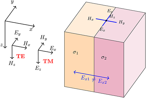
In the context of magnetotellurics, the propagation of electromagnetic plane waves in the Earth can be described by two fundamental modes, depending on the orientation of the electric and magnetic fields. The transversal electric (TE) and transversal magnetic (TM) modes, presented in Figure 5.
The TE mode occurs for the electric field -component, that is, , while the magnetic field has components in the and directions, that is, . The TM mode arises when the electric field has the and -component, that is, , while the magnetic field has components in the direction, that is, .
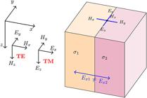
Two types of wave propagation in a two-dimensional Earth model. TE mode (left) and TM mode (right).
10. One-Dimensional Earth
In a 1D model, the conductivity depends only on the depth. The incidence of electromagnetic waves is assumed to be vertical (plane waves), and the fields decouple in the TE and TM modes. In the 1D model, the components of obey the following relationships, where .
10.1. Equations to TE mode
From Eq. (12) and considering the vectors and , then
Then,
According to Faraday’s law, Eq. (12) is described by:
and how electric field only depends from depth, , so we have
From Eq. (13) and considering a quasi-static condition (assumes that at low frequencies the displacement current term is negligible compared to the conduction current), where and how magnetic field only depends from depth, we obtain:
Differentiating Eq (67) with respect to , we obtain:
Substituting into the expression above:
This yields a second-order differential equation, in which the complex wave number is defined as . The equation becomes:
This is a homogeneous linear second-order differential equation with constant coefficients. The general form of such an equation is:
The general solution is:
Solving the characteristic equation:
Thus, the solution for the electric field is:
To determine , we use the relation:
Differentiating Eq. (76) with respect to :
Substituting into the expression for :
The magnetotelluric impedance is defined as:
Since electromagnetic waves attenuate with depth in a conductive medium, the exponentially increasing solution must be discarded to avoid unphysical divergence as . Therefore:
Substituting the definition of , we obtain:
The apparent resistivity is then given by:
Thus, the expression for the apparent resistivity becomes:
Finally, the phase of the impedance, which quantifies the phase shift between the electric and magnetic fields, is defined by:
10.2. Equations to TM mode
From Eq. (12) and considering the vectors and then,
Then,
how electric field only depends on depth, , so we have:
From Eq. (13) and considering a quasi-static condition where ,then , we get:
According to Ampere’s law, Eq. (13),
As the magnetic field only depends on depth, we have,
Differentiating Eq. (88) with respect to , we get
Replacing and reordering the equation,
Again, we have a differential equation with constant coefficients of the second order with . Then,
To find , we can use Eq. (88):
Differentiating Eq. (95) with respect to ,
The impedance is defined as:
Considering is nullified, then,
Thus, we have,
The apparent resistivity follows the same form:
The phase of the impedance is identical to Eq. (85).
11. Recurrence Formulas for Impedance in 1D Earth Models
A variety of equations have been developed to solve 1D magnetotelluric models. These equations primarily compute the transfer function (impedance) at the top of the N-th layer. The solution is obtained iteratively, starting from the bottom layer, which is assumed to be a homogeneous half-space. The solution is then recursively propagated upward through the overlying layers until it reaches the surface.
This article presents three of these equations. Additionally, all of them are accompanied by Python code, which is available on GitHub, to facilitate a better understanding of the underlying physical modeling. The program can be downloaded from link: here.
11.1. Wait recursion (1954)
Wait [7] criticizes the validity of Cagniard [2] analysis of the behavior of telluric currents, refining the conditions under which the concept of field impedance is valid. Wait [7] affirms that the harmonic components of the electric field and the magnetic field tangential to the ground are only proportional to one another if the fields are sufficiently slowly (not changing abruptly from one point to another) varying over the surface of the ground. The visualization of the medium, the distribution of physical properties and the model parameters is shown on Figure 6.
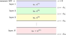
Wait results were extended to include the effects of a layered ground with both conductivity and susceptibility variations. Finally, the corresponding transient problem for a two-layer horizontally stratified earth is solved, and a general equation for N-layers could be derived.
We have two types of impedance , the intrinsic which is the impedance from an homogeneous medium which only depends from the properties of the layer and the entry that represents the impedance from the top of the -layer. Other properties from equations are: the conductivity , the permittivity , the subsurface propagation constant, here namely and the angular frequency , described by Eq. (103), from which we use frequency so,
The other one is the entry impedance
Wait’s recursion compute the impedance at the top of the N-th layer. The equation is solved iteratively, starting from the bottom layer, which is assumed to be a homogeneous half-space, and recursively propagating the solution upward through the overlying layers until the surface.
11.2. Constable recursion (1987)
Constable [8] introduced an alternative recursive formulation for calculating the MT impedance, in which the quantity , somewhat informally referred to as the “complex C value”, represents the layer-to-layer impedance response. This approach provides a natural and direct means of expressing MT data in terms of impedance. The recursion is defined as:
where is the complex wave number for layer , with denoting the electrical resistivity of layer (in ) and representing its thickness (in meters).
11.3. Grandis recursion (1999)
Grandis [9] proposed an alternative algorithm for one-dimensional magnetotelluric response calculation. Instead of using the classical recursive formula that directly relates the impedance at the surface of two successive layers, the proposed method employs a recursive formulation based on the electromagnetic fields at the top of two consecutive layers. This approach leads to a matrix multiplication scheme that offers improved numerical stability and flexibility in certain computational scenarios.
The surface impedance , representing the magnetotelluric response at the Earth’s surface, is calculated from the elements of the total transfer matrix , which encapsulates the cumulative effect of all subsurface layers. This total transfer matrix is obtained by sequentially multiplying the individual transfer matrices associated with each of the finite layers in the model:
where each relates the electromagnetic fields across the -th layer. The final expression for the surface impe-dance is given by:
where are the elements of the total transfer matrix , and is the intrinsic impedance of the -th layer, modeled as a homogeneous half-space extending to infinity.
The original implementation of the algorithm was developed in Fortran 77. For the purpose of study and analysis, it was translated into Python 3.8.
12. Sintetic Application
To demonstrate the application of the modeling codes and analyze their responses, we applied them to a synthetic model illustrated in Figure 7. The corresponding results are presented in Figure 8. All modeling approaches yielded identical response curves, reinforcing the consistency and reliability of the implemented methods.

Synthetic 1D model of physical properties (resistivity) used in magnetotelluric simulations.

13. Conclusions
The basic theory of the magnetotelluric (MT) method was presented, covering fundamental concepts such as signal sources, frequency range, and boundary conditions. The development of the method’s core equations began with Maxwell’s curl equations in the frequency domain and proceeded step by step, incorporating key concepts such as constitutive relations, diffusion equations, skin depth, and the specific characteristics of the impedance tensor.
The one-dimensional (1D) case we also discussed leading to analytical expressions for the impedance, where , as well as for the apparent resistivity and phase shift. Furthermore, three classical formulations for 1D modeling were presented: the recursive approaches of Wait, Constable, and Grandis. In support of teaching and learning, these methods were implemented in Python, providing practical tools to help students and educators bridge the gap between theoretical derivations and computational applications.
Data Availability
All the data supporting the results of this study were published in the article itself.
Referências
- [1] A.N. Tikhonov, Doklady 73, 295 (1950).
- [2] L. Cagniard, Geophysics 18, 605 (1953).
- [3] S. Constable, Geophysics 75, 75A67 (2010).
- [4] K. Vozoff, Geophysics 37, 98 (1972).
- [5] M.N. Nabighian (ed.), Electromagnetic methods in applied geophysics: Volume 1, Theory (Society of Exploration Geophysicists, Tulsa, 1988).
- [6] D.J. Griffiths, Eletrodinâmica (Pearson Addison-Wesley, São Paulo, 2011).
- [7] J.R. Wait, Geophysics 19, 281 (1954).
- [8] S.C. Constable, R.L. Parker and C.G. Constable, Geophysics 52, 289 (1987).
- [9] H. Grandis, Computers & Geosciences 25, 119 (1999).
Edited by
-
Editor-in-Chief:
Marcello Ferreirahttps://orcid.org/0000-0003-4945-3169