The Sommerfeld-Watson transformation in teaching condensed matter physics: analytical diagonalization of Fermi gas-like models

Abstract

This work presents the application of the lesser-known yet significant Sommerfeld-Watson transformation (SWT) for the analytical diagonalization of specific Hamiltonians in condensed matter physics. This powerful mathematical technique is particularly useful for simplifying summations over discrete quantum numbers by converting them into contour integrals in the complex plane. We focus on the Fermi gas and the non-interacting single-impurity Anderson model, both fundamental for describing important phenomena such as electronic conductance in metals, x-ray photoemission, and aspects of the Kondo problem. A comprehensive explanation of the SWT is provided, and its role in the diagonalization of these models is illustrated using modern notation for enhanced clarity. The analytical results obtained were validated against direct numerical diagonalization, showing excellent agreement. Additionally, we extended the method to a generalized version of the non-interacting single-impurity Anderson model, incorporating variable couplings and an arbitrary band dispersion, and provided two non-trivial examples. The procedure successfully achieved the analytical diagonalization of this more complex model, offering a generalized solution not previously reported in the literature. The detailed presentation, modern notation, and numerical validation of the SWT applied to key models in condensed matter physics constitute a valuable pedagogical resource, enriching the teaching of theoretical condensed matter physics.

Keywords
Sommerfeld-Watson transformation; analytical Diagonalization; Fermi gas-like models; condensed matter physics

1. Introduction

The Sommerfeld-Watson transformation (SWT) is a mathematical technique used to convert a series to a contour integral in the complex plane, simplifying its evaluation [¹, ²]. Such series naturally arise in problems involving discrete quantum numbers, for example, in scattering theory [³,⁴,⁵,⁶], where sums over poles or discrete quantum states are common. This technique is also applied in the analysis of amplitudes in high-energy physics [⁷, ⁸], in the study of many-particle scattering theory [⁹], and is frequently employed in quantum field theory, particularly in the analysis of spectral functions [¹⁰]. It can also be applied to electrostatic problems, where sums over discrete functions are common [¹¹,¹²,¹³,¹⁴]. Undoubtedly, it is a highly versatile method that enriches the analytical toolkit of theoretical physicists.

A lesser-known application of the SWT is its role in the analytical diagonalization of important and widely studied Hamiltonians in condensed matter physics, such as the Fermi gas Hamiltonian and the single-impurity Anderson model (SIAM) [¹⁵] in the non-interacting limit, where the Coulomb repulsion is neglected. Since the understanding of these models often relies on their diagonalization, this further demonstrates the utility of this transformation.

The Fermi gas model, for instance, describes the many-body behavior of non-interacting fermions. It is particularly relevant for studying metallic bands dominated by the superposition of s and p orbitals [¹⁶], where Coulomb interactions can be ignored. Despite its apparent simplicity, a Fermi gas under a localized scattering potential captures a variety of important physical phenomena, including electrical conductance in metals [¹⁶], x-ray emission and absorption [¹⁷,¹⁸,¹⁹,²⁰,²¹], and the x-ray photoemission [²²,²³,²⁴,²⁵,²⁶,²⁷].

The SIAM, on the other hand, describes a magnetic impurity coupled to a non-interacting Fermi gas [¹⁵]. It accounts for phenomena such as Kondo physics [²⁸,²⁹,³⁰] and the behavior of single-electron transistors [³¹], among others. In general, this model cannot be diagonalized exactly [¹⁶]. However, it can be solved in the non-interacting limit, which permits the analysis of fixed-point Hamiltonians within Renormalization Group theory [³²], playing a fundamental role in the Fermi-liquid description of the Kondo problem [²⁸,²⁹,³⁰].

The Fermi gas and the non-interacting SIAM have already been diagonalized using SWT-based methods (see Refs. [²⁶, ²⁸]). However, these works often omit relevant mathematical details or rely on outdated notations. For example, Refs. [²⁶, ²⁸, ²⁹] present only the final results, assuming the reader is already familiar with the diagonalization procedure. While it is possible to reconstruct the calculations, a more detailed derivation would significantly enhance comprehension.

In this paper, we aim to demonstrate the generalization of the diagonalization procedure based on the SWT, extending its application from simple models to a broader class of more complex quadratic Hamiltonians. To this end, we provide a detailed, self-contained presentation of the SWT, which is not always readily available in the literature, and highlight its role in the analytical diagonalization of two well-known examples: the Fermi gas under a localized scattering potential and the non-interacting SIAM. Moreover, for these examples, we compare the analytical solutions with numerical results obtained through brute-force diagonalization, finding excellent agreement between the two approaches.

We also consider a more general version of the non-interacting SIAM, in which no specific band dispersion is assumed and the couplings are allowed to vary. We present a unified analytical solution for this generalized non-interacting SIAM, from which the solutions for simpler cases can be recovered. To the best of our knowledge, this general analytical solution has not been previously derived. Additionally, we provide two non-trivial examples with numerical validation. Despite the increased mathematical complexity, we show that the same diagonalization procedure remains effective in this broader case.

We believe this detailed presentation of the Sommerfeld-Watson transformation will serve as a valuable pedagogical tool for analyzing and teaching a wide range of problems in condensed matter physics. In addition, the generalized solution presented here can be applied to study the properties of more complex and realistic Fermi gas-like systems.

This article is organized as follows: In Section 2, we outline the diagonalization procedure based on the SWT and present the general form of the Hamiltonian required for this approach. In Sections 3 and 4, we apply this procedure to two well-known examples: the Fermi gas and the non-interacting SIAM. Section 5 compares the results obtained in Sections 3 and 4 with numerical diagonalization. In Section 6, we introduce a generalized non-interacting SIAM and present its analytical diagonalization. Two non-trivial examples, supported by numerical validation, are presented. Finally, Section 7 summarizes our conclusions.

2. The Diagonalization Procedure

Here, we outline the key steps for analytically diagonalizing certain types of Hamiltonians using the Sommerfeld-Watson transformation. The following sections apply these general ideas explored to well-known examples. The diagonalization procedure applies to any quadratic fermionic Hamiltonian that can be expressed in the second quantization formalism [¹⁶, ³⁸] as

(1) $$\widehat{H}={\displaystyle \sum _k{\epsilon }_k}{\widehat{c}}_k^{†}{\widehat{c}}_k+{\displaystyle \sum _{k,q}\left(M_k{\overline{M}}_q+M_q^{*}{\overline{M}}_k^{*}\right)}{\widehat{c}}_k^{†}{\widehat{c}}_q.$$

${\widehat{c}}_k^{†}$ (${\widehat{c}}_k$) are the creation (annihilation) operators for fermions with energy ε_k, where k identifies the possible energy levels of the system, which resembles the Fermi gas. Note that the product of the independent terms M_k and ${\overline{M}}_q$ represents the couplings between the fermionic states (off-diagonal terms), and “*” denotes the complex conjugation. Although the requirement that the coupling takes the form $M_k{\overline{M}}_q$ may initially seem overly restrictive, it accommodates a broad class of models, including those of interest described by the Hamiltonians in Refs. [²⁴, ²⁶,²⁷,²⁸,²⁹,³⁰, ³³].

Here, we will focus on one-dimensional Hamiltonians, where k is a scalar. However, this procedure can also be adapted to higher-dimensional Hamiltonians with couplings $M_{\overrightarrow{k}}{\overline{M}}_{\overrightarrow{q}}$. While the summation and the resulting expressions may become more complicated in higher dimensions, it remains feasible. The simpler higher-dimensional case is when the energy depends only on $k=|\overrightarrow{k}|$ (spherical symmetry in d dimensions), converting the sums ${\Sigma }_{\overrightarrow{k}}$ into sums over k [¹⁶].

Similar steps can be adapted to diagonalize bosonic Hamiltonians with a form similar to equation (1); however, some sign differences may appear throughout the calculations presented here. In the following, we outline the procedure for diagonalizing the Hamiltonian in equation (1) for a large number of fermionic states, which can be interpreted as a Fermi gas-like model (diagonal terms) subject to a perturbation (off-diagonal terms).

2.1. First step: the Ansatz

A diagonal Hamiltonian in second quantization can be written as

(2) $$\widehat{H}={\displaystyle \sum _m{ϵ}_m}{\widehat{g}}_m^{†}{\widehat{g}}_m,$$

where {ϵ_m} are its eigenvalues and $\{{\widehat{g}}_m^{†}\}$ one-particle eigenoperators of the Hamiltonian, which creates a fermion with energy ϵ_m. Diagonalizing the Hamiltonian (1) means finding the sets of energies {ϵ_m} and single-particle operators $\{{\widehat{g}}_m^{†}\}$ such that it can be compressed in the above form. Since the initial set of operators forms a complete vector space, the operator ${\widehat{g}}_m^{†}$ can be written as a linear combination of the initial ones $\{{\widehat{c}}_k^{†}\}$ as

(3) $${\widehat{g}}_m^{†}={\displaystyle \sum _k{u}_{k,m}}{\widehat{c}}_k^{†}.$$

Here, u_k,m are the coefficients of the mentioned linear combination, which we aim to find in the diagonalization procedure¹.

2.2. Second step: computing the commutators

In this step, we compute the commutators $[H,{\widehat{c}}_k^{†}]$ and $[H,{\widehat{g}}_m^{†}]$ using equations (1), (2) and (3). This computation is crucial as it enables us to derive a system of coupled equations, whose solutions are the eigenvalues and eigenstates of the Hamiltonian, as will become clearer in the next step. After some manipulations following the calculations shown in Appendix A, we find

(4) $$[\widehat{H},{\widehat{c}}_k^{†}]=\left[{\epsilon }_k{\widehat{c}}_k^{†}+{\overline{M}}_k{\displaystyle \sum _q{M}_q}{\widehat{c}}_q^{†}+M_k^{*}{\displaystyle \sum _q{\overline{M}}_q^{*}}{\widehat{c}}_q^{†}\right],$$

and

(5) $$[\widehat{H},{\widehat{g}}_m^{†}]={ϵ}_m{\widehat{g}}_m^{†}.$$

In the next step, we use these commutation relations to derive equations that determine the eigenvalues and eigenoperators of the Hamiltonian (1).

2.3. Third step: the eigenenergies andeigenoperators equations

This step involves extensive manipulation of the above equations and more complex mathematical derivations, which we avoid at this point. All details are explicitly presented in Appendix B. Instead, we will summarize here the main steps, which consist of manipulating equations (3), (4), and (5), resulting in the expression

(6) $${\left|1-{\displaystyle \sum _k\frac{{\overline{M}}_k{M}_k}{{ϵ}_m-{\epsilon }_k}}\right|}^2={\displaystyle \sum _k\frac{|M_k{|}^2}{{ϵ}_m-{\epsilon }_k}}{\displaystyle \sum _k\frac{|{\overline{M}}_k{|}^2}{{ϵ}_m-{\epsilon }_k}}.$$

Equation (6) represents the eigenvalue equation, and its solutions, {ϵ_m}, correspond to the eigenvalues of the Hamiltonian. A similar coupled equation involving these summations can be used to determine the coefficients u_k,m (see Appendix B). This is precisely where the Sommerfeld-Watson transformation becomes highly useful, in the sense that it simplifies the sums,

(7) $$\begin{array}{c}S(ϵ)={\displaystyle \sum _k\frac{|M_k{|}^2}{ϵ-{\epsilon }_k}},\overline{S}(ϵ)={\displaystyle \sum _k\frac{|{\overline{M}}_k{|}^2}{ϵ-{\epsilon }_k}},\text{and}\\ \tilde{S}(ϵ)={\displaystyle \sum _k\frac{M_k{\overline{M}}_k}{ϵ-{\epsilon }_k}}.\end{array}$$

After this, the equation ${\left|1-\tilde{S}(ϵ)\right|}^2=S(ϵ)\tilde{S}(ϵ)$ can be solved and the eigenvalues of $\widehat{H}$ determined.

2.4. Last step: the Sommerfeld-Watsontransformation

To complete the diagonalization, we address the sums in equation (7). Here, we focus on Fermi gas-like systems with a large number of particles, where these sums take the general form of

(8) $$S={\displaystyle \sum _{n=-\infty }^{\infty }f}(n),$$

where f(n) is a function defined for discrete integers n.

The SWT replaces this summation with the evaluation of a complex integral through the following steps². First, let us consider the complex function F(z) = πf(z) cot⁡(πz), where z ∈ ℂ. F(z) has simple poles in the set of integer values {n} arising from the term cot⁡(πz). The function can also have other poles coming from f(z) denote by {z₀}, which, for simplicity, we consider z₀ ∉ ℤ. Therefore, employing the residue theorem [³⁴], we can define a contour integral in the complex plane:

(9) $$\begin{array}{l}\frac{1}{2i}{\displaystyle {\oint }_{C}f(z)\cot (\pi z)}dz\\ ={\displaystyle \sum _{n=-\infty }^{\infty }f}(n)+\pi {\displaystyle \sum _{\left\{z_0\right\}}\cot }(\pi z_0)\text{Res}(f(z),z=z_0),\end{array}$$

where the original sum we seek to evaluate in equation (8) appears among the residue terms. Here, the contour C is an arbitrary-closed contour in the complex plane that includes all integers, as shown in Fig. 1, and {z₀} denotes all poles of f(z) within C, and we use the simple pole residue formula [³⁴], that is,

Figure 1
A few examples of appropriate contours for evaluating the Sommerfeld-Watson transformation are shown. The blue lines (solid and dashed) represent examples of suitable closed contours, while the black “×” symbols indicate the integer poles and the red “×” symbols denote the poles of the function f(z). The latter poles do not necessarily need to be inside the contour.

(10) $$\begin{array}{l}\underset{z\to n}{\lim }f(z)\cot (\pi z)\cdot (z-n)\\ =\underset{z\to n}{\lim }f(z)\cos (\pi z)\frac{(z-n)}{\sin (\pi z)}=\frac{1}{\pi }f(n).\end{array}$$

Moreover, by rearranging the equation (9), we obtain

(11) $$\begin{array}{c}{\displaystyle \sum _{n=-\infty }^{\infty }f}(n)=\frac{1}{2i}{\displaystyle {\oint }_{C}f}(z)\cot (\pi z)dz\\ -\pi {\displaystyle \sum _{\left\{z_0\right\}}\cot }(\pi z_0)\text{Res}(f(z),z=z_0).\end{array}$$

To compute the integral on the right-hand side, we have to choose an appropriate contour C. The interpretation of equation (11) is straightforward: the first term on the right-hand side accounts for the contribution from the sum far away from the poles, while the second term captures the contributions around the poles.

As an simple example of the SWT applications, let us consider a small modification of the Bessel problem ${\sum }_{n\ge 1}{n}^{-2}=\frac{{\pi }^2}{6}$, given by

(12) $$S={\displaystyle \sum _{n=-\infty }^{\infty }\frac{1}{n^2+{\eta }^2}}\stackrel{\text{SWT}}{=}\frac{1}{2i}{\displaystyle {\oint }_C\frac{\cot (\pi z)}{z^2+{\eta }^2}}dz-\frac{\pi \cot (\pi i\eta )}{i\eta }.$$

Here, we used the SWT in equation (11) considering the poles z₀ ∈ {−iη, iη}.

We can now choose the circular integration path shown in Fig. 1 in the |z| → ∞ limit to eliminate the contribution of the first term on the right-hand side of equation (12)³. Using the identity $\cot (ix)=-i\times \frac{\cosh (x)}{\sinh (x)}$, it is straightforward to show that equation (12) simplifies to

(13) $${\displaystyle \sum _{n=-\infty }^{\infty }\frac{1}{n^2+{\eta }^2}}=\frac{\pi }{\eta }\frac{\cosh (\pi \eta )}{\sinh (\pi \eta )},$$

and finally prove that

(14) $$\begin{array}{ll}{\displaystyle \sum _{n=1}^{\infty }\frac{1}{n^2}}\hfill & ={\left[{\displaystyle \sum _{n=1}^{\infty }\frac{1}{n^2+{\eta }^2}}\right]}_{\eta =0}\hfill \\ \hfill & =\underset{\eta \to 0}{\lim }\left[-\frac{1}{2{\eta }^2}+\frac{\pi }{2\eta }\frac{\cosh (\pi \eta )}{\sinh (\pi \eta )}\right]=\frac{{\pi }^2}{6}.\hfill \end{array}$$

Small modifications to the presented transformation can be applied in other contexts. For example, by defining the function F(z) = πf(z)/sin⁡(πz), one can address alternating series. In addition, the choice of the complex contour C is arbitrary. A circular contour is especially appropriate for functions f(z) with fast decay (f(|z| ≫ 1) ∼ |z|⁻² or faster), such as the Bessel problem $S={\sum }_{n\ge 1}{n}^{-2}=\frac{{\pi }^2}{6}$, where the contribution vanishes as the radius R → ∞[³⁵].

Although there is no recipe for performing the SWT, the procedure typically begins by defining the function F(z) = πf(z) cot⁡(πz) (or F(z) = πf(z)/sin⁡(πz) for alternating sums). This formulation isolates the poles of sin⁡(πz) from those of f(z), facilitating the extraction of the sum S. The next steps involve selecting an appropriate closed complex contour, computing the residues of f(z), and deriving an expression for S. In the following sections, we present two examples to illustrate the application of this method in condensed matter physics.

3. Fermi Gas Under a Localized Scattering Potential

In this section, we diagonalize the Hamiltonian of a Fermi gas in the presence of a localized scattering potential. This model describes non-interacting fermions (a Fermi gas), such as electrons in a simple metal, subjected to a localized perturbation [³³], which could represent a frozen impurity, a localized external electric potential, or a charged particle near the Fermi gas. Since this perturbation is external to the Fermi gas, it acts as a scattering mechanism, altering the momentum of each fermion in the system [¹⁶]. A good example of such a mechanism is the ionization of deep-core atoms when a metal is struck by x-rays, leaving behind a localized positive charge that acts as a scattering potential for the conduction electrons [¹⁶,¹⁷,¹⁸,¹⁹, ²¹, ²²].

Despite its simplicity, this model has played a crucial role in the development of new ideas [³³] and in explaining fascinating phenomena in metals such as x-ray photoemission, leading to x-ray photoemission spectroscopy [³⁶], and x-ray absorption and emission, leading to x-ray absorption spectroscopy [³⁷]. The diagonalization of this Hamiltonian is the essential first step in understanding how the presence of a localized scattering potential perturbs the Fermi gas (or a simple metal) [¹⁶,¹⁷,¹⁸,¹⁹, ²¹,²²,²³,²⁴,²⁵,²⁶,²⁷], and consequently, the aforementioned phenomena.

3.1. The Hamiltonian

Let us begin with a simpler version: the spinless Hamiltonian $\widehat{H}$ in second quantization notation [¹⁶, ³⁸], which describes a spinless Fermi gas under a localized scattering potential of strength W (an external charged particle or electric field, for example). It is given by

(15) $$\widehat{H}={\displaystyle \sum _k{\epsilon }_k}{\widehat{a}}_k^{†}{\widehat{a}}_k+\frac{W}{2L}{\displaystyle \sum _{k,q}{\widehat{a}}_k^{†}}{\widehat{a}}_q,$$

where ${\widehat{a}}_k^{†}$ (${\widehat{a}}_k$) are the creation (annihilation) operators for fermions in the momentum state k, 2L is the number of states, ε_k is the energy dispersion relation, and W is the amplitude of the localized scattering potential.

In equation (15), the Hamiltonian is written in momentum space (k-space). The first term on the right-hand side corresponds to the effective kinetic energy of each fermion in the Fermi gas, while the second term accounts for the scattering due to the localized potential of strength |W|. It is important to note that “localized”, as used here, refers to real space. Since the Hamiltonian is expressed in momentum space, something localized in real space appears as a spread across all k values in momentum space, as represented by the second term on the right-hand side.

For simplicity, we will consider ε_k = Δ ⋅k, a linear dispersion relation, where Δ is the difference between two consecutive energy levels and k is an integer such that −L ≤ k ≤ + L. As already mentioned, our focus here is on one-dimensional systems, where k is a scalar.

The energy spectrum of a Fermi gas system is limited by a maximum energy value that depends on the characteristics of the model [¹⁶], called the bandwidth energy D. Then, for a large number of energy levels, we have Δ → 0, approaching a gapless band.

In our model, we consider the bandwidth energy of the fermionic levels as D = Δ ⋅ L. As a result, the fermionic density of states, which accounts for the proportion of the total number of energy levels that exist per unit of energy, mathematically described by

(16) $$\rho \equiv \frac{1}{2D}=\frac{1}{(2L\Delta )}.$$

These definitions will prove useful in future calculations.

3.2. Analytical diagonalization of the model

As mentioned in the previous section, the diagonal form of $\widehat{H}$ is described by equation (2), where the operator ${\widehat{g}}_m^{†}$ can be written as a linear combination of the initial band operators $\{{\widehat{a}}_k^{†}\}$ as

(17) $${\widehat{g}}_m^{†}={\displaystyle \sum _k{u}_{k,m}}{\widehat{a}}_k^{†}.$$

Our task now is to determine the eigenvalues {ϵ_m} and the “eigenvectors” coefficients {u_k,m}. Then, the second step of the procedure continues by computing $[\widehat{H},{\widehat{a}}_k^{†}]$ and $[\widehat{H},{\widehat{g}}_m^{†}]$. After some manipulations assisted by the result in Appendix A, we arrive at the following expressions:

(18) $$[\widehat{H},{\widehat{a}}_k^{†}]={\epsilon }_k{\widehat{a}}_k^{†}+\frac{W}{2L}{\displaystyle \sum _q{\widehat{a}}_q^{†}}$$

and $[\widehat{H},{\widehat{g}}_m^{†}]={ϵ}_m{\widehat{g}}_m^{†}$, as shown by equation (5).

By substituting ${\widehat{g}}_m^{†}$ on both sides of equation (5) using its expansion in terms of the operators $\{{\widehat{a}}_k^{†}\}$ defined in equation (17), and after some algebraic manipulations, we get

(19) $${\displaystyle \sum _k\left[{\epsilon }_k{u}_{k,m}+\frac{W}{2L}{\displaystyle \sum _q{u}_{q,m}}\right]}\mathrm{}{\widehat{a}}_k^{†}={\displaystyle \sum _k{ϵ}_m}{u}_{k,m}{\widehat{a}}_k^{†}.$$

As the operators ${\widehat{a}}_k^{†}$ are linearly independent, each term of the k-sum above must satisfy the equation independently, resulting in

(20) $$\left({ϵ}_m-{\epsilon }_k\right)u_{k,m}-\frac{W}{2L}{\displaystyle \sum _q{u}_{q,m}}=0.$$

Isolating the term u_k,m and summing over all possible k-states, we can write

(21) $${\displaystyle \sum _k{u}_{k,m}}=W\left(\frac{1}{2L}{\displaystyle \sum _k\frac{1}{\left({ϵ}_m-{\epsilon }_k\right)}}\right){\displaystyle \sum _q{u}_{q,m}}.$$

Considering ∑_k u_k,m ≠ 0, it is straightforward to show that we obtain the following condition

(22) $$1=W\left(\frac{1}{2L}{\displaystyle \sum _k\frac{1}{\left({ϵ}_m-{\epsilon }_k\right)}}\right).$$

This expression is the eigenvalue equation of the Fermi gas system, and its solution will provide the missing eigenenergies {ϵ_m}.

Keeping that in mind, we aim now to analyze the sum on the right-hand side of equation (22). For this reason, it is convenient to define a new variable S_m as

(23) $$S_m=\frac{1}{2L}{\displaystyle \sum _q\frac{1}{{ϵ}_m-{ϵ}_q}}.$$

The final step is to use the Sommerfeld-Watson transformation to find an explicit formula for S_m. But before proceeding, it is important to note that the scattering potential W in the Hamiltonian $\widehat{H}$ shifts each initial eigenvalue ε_m by a certain amount of energy. For reasons that will become clear in the following calculations, we define this energy shift as $\left(-\frac{{\delta }_m}{\pi }\right)\mathrm{\Delta }$, where δ_m is the phase shift and Δ is the difference between two consecutive energy levels near the Fermi energy. In principle, δ_m can take any value that adjusts the initial eigenvalue to match the eigenvalue ϵ_m in the presence of the scattering potential. In this situation, we can write the final energies as

(24) $${ϵ}_m={\epsilon }_m-\frac{{\delta }_m}{\pi }\mathrm{\Delta }.$$

Now, recalling that ε_k = Δ ⋅ k, and using equations (24) and (16), it is straightforward to show that the summation S_m given by the equation (23) can be rewritten as

(25) $$S_m=-\rho {\displaystyle \sum _q\frac{1}{q-m+\frac{{\delta }_m}{\pi }}}.$$

Following last step of the diagonalization procedure, discussed in section 2, we write the sum as S_m = ρ∑_n f(n) with f(z) = −(z − z₀)⁻¹, a function with a single simple pole at z₀ = m − δ_m/π. After the SWT defined by equation (11), the sum S_m in equation (25) transform into

(26) $$S_m=-\frac{1}{2i}{\displaystyle {\oint }_C\frac{dz\rho \text{cot}(\pi z)}{z-\left(m-\frac{{\delta }_m}{\pi }\right)}}+\pi \rho \text{cot}(\pi m-{\delta }_m).$$

The last term on the right-side of equation (26) can be simplified to cot⁡(πm − δ_m) = −cot⁡(δ_m). We now only need an expression for the complex integral. For this purpose, it is necessary to define a closed contour C in the domain of the function F(z) = f(z)cot(z). An appropriate complex contour for this problem is shown in Fig. 2 (left panel), once lim_{(Imz→±∞)} cot (Re(z) + i Im (z)) = ∓i. Taking the limit where the box size shown in Fig. 2 tends to infinity, we write

Figure 2
(Left panel) Integration path of (26), a square in the complex domain centered at the origin with size L. (Right panel) Auxiliary path to simplify the integral over C. In the upper and bottom boundaries of the integration path C, it is true that lim_{(Imz→±∞)} cot (Re(z) + i Im (z)) = ∓i, which results in the expression in equation (30). The integration contours shown here run in the counterclockwise direction.

(27) $$\frac{1}{2i}{\displaystyle {\oint }_{C}d}z\frac{\text{cot}(\pi z)}{z-\left(m-\frac{{\delta }_m}{\pi }\right)}=-\frac{1}{2}\underset{y\to +\infty }{\lim }{\displaystyle {\int }_{+\infty }^{-\infty }d}x\frac{1}{x+iy-z_0}+\frac{1}{2}\underset{y\to -\infty }{\lim }{\displaystyle {\int }_{-\infty }^{+\infty }d}x\frac{1}{x+iy-z_0}.$$

Using an auxiliary path, shown in the right panel of Fig. 2, for a function f(z) with poles only in the real axis, it is true that $\frac{1}{2i}{\oint }_{\pm }f(z)\mathit{d}z=0$. Moreover, the following statement holds

(28) $$\underset{y\to \pm \infty }{\lim }{\displaystyle {\int }_{+\infty }^{-\infty }d}x\frac{1}{x+iy-z_0}=-\underset{L\to \infty }{\lim }\underset{y\to 0^{\pm }}{\lim }{\displaystyle {\int }_{-L}^{+L}d}x\frac{1}{x+iy-z_0}.$$

Therefore, with the results in equations (27) and (28), we find that the total contribution from the closed path in Fig. 2 to S_m is simply

(29) $$𝒫{\int }_{-L\mathrm{\Delta }}^{+L\mathrm{\Delta }}d\epsilon \frac{\rho }{{\epsilon }_m-\epsilon },$$

where 𝒫 represents the Cauchy principal value of the integral. Then, the expression in equation (26) is rewritten as

(30) $$S_m=-\pi \rho \text{cot}({\delta }_m)+\rho 𝒫{\displaystyle {\int }_{-L\mathrm{\Delta }}^{+L\mathrm{\Delta }}\frac{d\epsilon }{{\epsilon }_m-\epsilon }}.$$

Finally, we find an explicit expression for S_m, and we can return to the diagonalization procedure.

From the identity W ⋅ S_m = 1 shown in equation (22), the direct substitution of S_m by its explicit expression shown in equation (30) leads to

(31) $$\begin{array}{lll}\cot ({\delta }_m)\hfill & =\hfill & \frac{1}{\pi }𝒫{\displaystyle {\int }_{-D}^{+D}\frac{1}{{\epsilon }_m-\epsilon }}d\epsilon -\frac{1}{\pi \rho W}+𝒪(\mathrm{\Delta })\hfill \\ \hfill & =\hfill & -\frac{1}{\pi \rho W}+\frac{1}{\pi }\ln \left(\frac{D+{\epsilon }_m}{D-{\epsilon }_m}\right).\hfill \end{array}$$

Our goal is to determine the new energy levels in the presence of the scattering potential. To achieve this, we need to compute the phase shift δ_m, which can be obtained from equation (31). From this expression, we can determine δ_m ≡ δ_m(ε_m, W) for each ε_m and fixed W, and consequently, find the eigenenergies using equation (24). To derive an explicit expression for the phase shift, we can rearrange equation (31) and show that the phase shift is given by

(32) $$\tan ({\delta }_m)=-\pi \rho W{\left(1-\rho W\ln \left(\frac{D+{\epsilon }_m}{D-{\epsilon }_m}\right)\right)}^{-1},$$

or, for the energy levels close to the Fermi energy, it can be approximated as

(33) $$\tan ({\delta }_m)\approx \tan ({\delta }_0)\equiv -\pi \rho W,$$

a constant that depends only on W, for |m| ≪ L. Here, we used the fact that $\ln \left(\frac{D+{\epsilon }_m}{D-{\epsilon }_m}\right)$ contributes on the order of 𝒪(m/L).

To complete the diagonalization of the Hamiltonian, we only have to find the coefficients u_k,m and, consequently, the eigenoperators $\{g_m^{†}\}$. We start by isolating the coefficient u_k,m in equation (20) and squaring both sides, and then applying the sum over k. This gives

(33a) $${\displaystyle \sum _k|u_{k,m}{|}^2}=\frac{W^2}{2L}\frac{1}{2L}{\displaystyle \sum _k\frac{1}{{\left({ϵ}_m-{\epsilon }_k\right)}^2}}{\left({\displaystyle \sum _q{u}_{q,m}}\right)}^2.$$

The normalization of the single particle state guarantees that ∑_k |u_k,m|² = 1 holds. Note that from equations (25) and (30), it is straightforward to show that

(34) $$-\frac{\mathrm{d}{S}_m}{\mathrm{d}{\mathrm{ϵ}}_m}=\frac{1}{2L}{\displaystyle \sum _k\frac{1}{{\left({ϵ}_m-{\epsilon }_k\right)}^2}}=\frac{1}{2L{\mathrm{\Delta }}^2}{\left|\frac{\pi }{\sin {\delta }_m}\right|}^2.$$

This leads to

(34a) $$1={\rho }^2{W}^2\left({\left|\frac{\pi }{\sin {\delta }_m}\right|}^2\right){\left({\displaystyle \sum _q{u}_{q,m}}\right)}^2,$$

or, after taking the square root,

(35) $${\displaystyle \sum _q{u}_{q,m}}=\pm \frac{\sin {\delta }_m}{\pi \rho W}.$$

Finally, substituting the equation (35) into the equation (20) we obtain the well-known form of the coefficients u_k,m as

(36) $$u_{k,m}=-\frac{\text{Δ}}{\left({ϵ}_m-{\epsilon }_k\right)}\frac{\sin {\delta }_m}{\pi },$$

and the energy eigenvalues ϵ_m from equations (24) and (32), completing the diagonalization procedure. The minus sign in equation (35) is chosen to ensure that ${lim}_{\delta \to 0}{u}_{k,m}={\delta }_{k,m}^K$, where ${\delta }_{k,m}^K$ represents the Kronecker delta [³⁸].

Equations (24), (32), and (36) can be used to derive the Anderson orthogonality catastrophe [²⁴, ³³], which states that the Fermi gas ground states before and after the introduction of a localized potential are orthogonal, even for small values of W. This catastrophe has profound consequences in condensed matter physics and is responsible for the power-law behavior observed in the x-ray photoemission, emission, and absorption spectra of metals (see Refs. [¹⁸, ²², ²⁶]).

4. The Non-Interacting Single Impurity Anderson Model

Another important model in condensed matter physics is the single-impurity Anderson model (SIAM) [¹⁵], which describes a magnetic impurity coupled to a non-interacting Fermi gas (or a metallic band). This model can explain the Kondo effect [³²], where an anomalous increase in the low-temperature resistivity of metals with a small concentration of magnetic impurities is observed, and it is extremely useful for understanding the behavior of quantum impurities coupled to a metallic wire [³⁹]. In particular, studies of the conductivity in such systems have led to the development of technological devices, such as the single-electron transistor [³¹].

In the second quantization, the SIAM can be described by the Hamiltonian

(37) $${\widehat{H}}_{\text{SIAM}}\equiv \left[{\epsilon }_d\left({\widehat{n}}_{d\uparrow }+{\widehat{n}}_{d\downarrow }\right)+U{\widehat{n}}_{d\uparrow }{\widehat{n}}_{d\downarrow }\right]+{\widehat{H}}_B+{\widehat{H}}_{\text{h}}.$$

The first term in brackets on the right-hand side is the contribution from the impurity, where ${\widehat{n}}_{d\sigma }={\widehat{d}}_{\sigma }^{†}{\widehat{d}}_{\sigma }$, and ${\widehat{d}}_{\sigma }^{†}$ (${\widehat{d}}_{\sigma }$) creates (annihilates) one electron in the impurity level with energy ε_d and spin σ = ↓, ↑. The Coulomb repulsion term U penalizes double occupancy. ${\widehat{H}}_B$ represents the Fermi gas, described by the Hamiltonian (15) with W = 0, and ${\widehat{H}}_{\mathrm{h}}$ is the hybridization and couples the impurity to the Fermi gas, allowing electron transfer between them.

Usually, it is a good approximation to consider that the impurity couples only to the neighboring metallic atoms. Then, in momentum space, the coupling is constant for all k values, and the hybridization term becomes:

(38) $${\widehat{H}}_{\text{h}}\equiv \frac{V}{\sqrt{2L}}{\displaystyle \sum _{k\sigma }\left({\widehat{a}}_{k\sigma }^{†}{\widehat{d}}_{\sigma }+{\widehat{d}}_{\sigma }^{†}{\widehat{a}}_{k\sigma }\right)},$$

where $\{{\widehat{a}}_{k\sigma }^{†}\}$ are the same fermionic creation operators defined in Section III, and V quantifies the strength of the impurity-Fermi gas coupling.

Despite the seemingly simple form of the SIAM defined in equation (37), the Coulomb interaction U makes the model non-quadratic, which cannot be diagonalized easily. To address the interacting case (U ≠ 0), more sophisticated approaches, such as the Bethe Ansatz [⁴⁰] or numerical methods like the Numerical Renormalization Group (NRG) [²⁵, ³⁹], the Real Space Numerical Renormalization Group (eNRG) [²⁶, ²⁹], and the Density Matrix Renormalization Group (DMRG) [³², ⁴¹,⁴²,⁴³], are required. However, these methods lie beyond the scope of this paper. Here, we will focus on analytically diagonalizing the simpler non-interacting SIAM (NI-SIAM), defined by setting U = 0. For this case, each spin component σ is completely independent of the others, and we can consider spinless fermions.

4.1. The NI-SIAM Hamiltonian

It is beneficial to introduce a small modification to the NI-SIAM to also account for the presence of a localized scattering potential W. In this case, the Hamiltonian can be written as

(39) $$\widehat{H}={\epsilon }_d{\widehat{d}}^{†}\widehat{d}+\frac{V}{\sqrt{2L}}{\displaystyle \sum _k\left({\widehat{d}}^{†}{\widehat{a}}_k+\text{H}.c.\right)}+{\displaystyle \sum _k{\epsilon }_k}{\widehat{a}}_k^{†}{\widehat{a}}_k+\frac{W}{2L}{\displaystyle \sum _{k,q}{\widehat{a}}_k^{†}}{\widehat{a}}_q,$$

which is also known as Newns-Anderson model [⁴⁴].

In summary, equation (39) is a Fermi gas-like model that describes a non-interacting impurity (first term) coupled to a Fermi gas (third term) under a localized scattering potential (fourth term), where the coupling is proportional to V and enables fermions to transfer between them (second term). This adjustment of the model allows the Hamiltonian to easily recover the pure NI-SIAM case by setting W = 0 (in the absence of a scattering potential), while also enabling its application to more general scenarios, such as the low-temperature Fermi liquid description of the Kondo effect [²¹, ²⁸,²⁹,³⁰]. Additionally, it allows one to recover the Fermi gas studied in Section 3 by setting V = 0, decoupling the impurity from the Fermi gas.

4.2. Analytical diagonalization of the NI-SIAM

Here, we aim to diagonalize the Hamiltonian (39). Similar to what was done in the Fermi gas problem, we can diagonalize this Hamiltonian if it is expressed in the form $\widehat{H}={\sum }_m{ϵ}_m{\widehat{g}}_m^{†}{\widehat{g}}_m$, where the operator ${\widehat{g}}_m^{†}$ is now

(40) $${\widehat{g}}_m^{†}={\displaystyle \sum _k{u}_{k,m}}{\widehat{a}}_k^{†}+u_{d,m}{\widehat{d}}^{†},$$

which is a linear combination of not only the Fermi gas operators $\{{\widehat{a}}_k^{†}\}$, but also the impurity operator ${\widehat{d}}^{†}$.

Following the diagonalization procedure described in Section II, we need to compute the commutators of $\widehat{H}$ with ${\widehat{g}}_m^{†}$, ${\widehat{a}}_k^{†}$ and ${\widehat{d}}^{†}$. Using the result from Appendix A to simplify the calculations, after some manipulations, we arrive at the following expressions:

(41) $$[\widehat{H},{\widehat{a}}_k^{†}]=\left[\frac{V}{\sqrt{2L}}{\widehat{d}}^{†}+{\epsilon }_k{\widehat{a}}_k^{†}+\frac{W}{2L}{\displaystyle \sum _q{\widehat{a}}_q^{†}}\right],$$

(42) $$[\widehat{H},{\widehat{d}}^{†}]=\left[{\epsilon }_d{\widehat{d}}^{†}+\frac{V}{\sqrt{2L}}{\displaystyle \sum _q{\widehat{a}}_q^{†}}\right],$$

and $[\widehat{H},{\widehat{g}}_m^{†}]={ϵ}_m{\widehat{g}}_m^{†}$, as shown by equation (5).

Using the equation (5) and substituting the operator ${\widehat{g}}_m^{†}$ expanded as the linear combination defined in (40), we arrive at

(43) $$\begin{array}{l}{\displaystyle \sum _k{ϵ}_m}{u}_{k,m}{\widehat{a}}_k^{†}+{ϵ}_m{u}_{d,m}{\widehat{d}}^{†}\\ ={\displaystyle \sum _k\left[{\epsilon }_k{u}_{k,m}+\frac{W}{2L}{\displaystyle \sum _q{u}_{q,m}}+\frac{V}{\sqrt{2L}}{u}_{d,m}\right]}{\widehat{a}}_k^{†}\\ +\left[{\epsilon }_d{u}_{d,m}+\frac{V}{\sqrt{2L}}{\displaystyle \sum _q{u}_{q,m}}\right]{\widehat{d}}^{†}.\end{array}$$

To derive the above expression, we used the results from equations (41) and (42).

Since each operator ${\widehat{a}}_k^{†}$ and ${\widehat{d}}^{†}$ in equation (43) are linearly independent, we can split the mentioned equation into two equalities as follows

(44) $$\left({ϵ}_m-{\epsilon }_k\right)u_{k,m}-\frac{W}{2L}{\displaystyle \sum _q{u}_{q,m}}=\frac{V}{\sqrt{2L}}{u}_{d,m},$$

and

(45) $$\left({ϵ}_m-{\epsilon }_d\right)u_{d,m}=\frac{V}{\sqrt{2L}}{\displaystyle \sum _q{u}_{q,m}}.$$

Similarly as the manipulations performed to diagonalize the Fermi gas, to solve the system of equations defined by (44) and (45), we can first isolate the term u_k,m in (44) and apply a sum over all possible values of k, resulting in

(46) $$\left[\text{}1-\frac{W}{2L}{\displaystyle \sum _k\frac{1}{{ϵ}_m-{\epsilon }_k}}\text{}\right]\text{}{\displaystyle \sum _q{u}_{q,m}}=\frac{V}{\sqrt{2L}}{\displaystyle \sum _k\frac{1}{{ϵ}_m-{\epsilon }_k}}{u}_{d,m}.$$

Isolating the term ∑_q u_q,m in equation (45) and substituting it into the equation (46) to find the following relation:

(47) $$({ϵ}_m-{\epsilon }_d)\left[1-\frac{W}{2L}{\displaystyle \sum _k\frac{1}{{ϵ}_m-{\epsilon }_k}}\right]=\frac{|V{|}^2}{2L}{\displaystyle \sum _k\frac{1}{{ϵ}_m-{\epsilon }_k}}.$$

Equation (47) defines an implicit equation for the eigenenergies {ϵ_m} of the NI-SIAM. Once again, we encounter the eigenvalue equation for the problem at hand. The next step is to solve this equation.

Keeping that in mind, we already know that the sum $S_m={\displaystyle \frac{1}{2L}}{\sum }_k{\displaystyle \frac{1}{{ϵ}_m-{\epsilon }_k}}$ can be computed by equation (30). Using this information in equation (47), the eigenvalues {ϵ_m} can implicitly be found through the expression

(48) $${ϵ}_m={\epsilon }_m-\frac{{\delta }_m}{\pi }\text{Δ}={\epsilon }_d+\frac{S_m|V{|}^2}{1-W{S}_m},$$

while S_m depending only on δ_m and the energy ε_m (that is, S_m = S_m(δ_m, ε_m)). More specifically, there are two equalities in the above expression:

(49) $${\epsilon }_m-\frac{{\delta }_m}{\pi }\text{Δ}={\epsilon }_d+\frac{S_m|V{|}^2}{1-W{S}_m},$$

which implicitly allows us to find the value of δ_m and ${ϵ}_m={\epsilon }_m-\frac{{\delta }_m}{\pi }\mathrm{\Delta }$, where we can find the eigenenergies {ϵ_m}.

Considering $|{\epsilon }_m-{\epsilon }_d|\gg \frac{|{\delta }_m|}{\pi }\mathrm{\Delta }$, after some mathematical manipulations, it is straightforward to show that the phase shift for the metallic levels can be obtained by

(50) $$\tan {\delta }_m\approx \tan {\delta }_m^{(0)}{\left(1+\frac{\tan {\delta }_m^{(0)}}{\pi }\ln \left(\frac{D+{\epsilon }_l}{D-{\epsilon }_l}\right)\right)}^{-1},$$

where

(51) $$\tan {\delta }_m^{(0)}=-\left[\pi \rho W+\frac{\pi \rho V^2}{{\epsilon }_m-{\epsilon }_d}\right].$$

To complete the diagonalization procedure, we now need to determine the coefficients u_k,m and u_d,m. The basis transformation must satisfy the normalization condition, ∑_k|u_k,m|² + |u_d,m|² = 1. To apply this condition, it is convenient to first express u_k,m in terms of u_d,m. One possible approach is to first isolate the term ∑_qu_q,m in equation (46) resulting in

(52) $${\displaystyle \sum _q{u}_{q,m}}=\frac{V}{\sqrt{2L}}{\left[1-\frac{W}{2L}{\displaystyle \sum _k\frac{1}{{ϵ}_m-{\epsilon }_k}}\right]}^{-1}\cdot {\displaystyle \sum _k\frac{1}{{ϵ}_m-{\epsilon }_k}}{u}_{d,m}.$$

Substituting the above relation into equation (44) and performing some algebraic manipulations, while keeping in mind the definition of S_m, we can rewrite the equation in the following form:

(53) $$u_{k,m}=\left[\frac{V}{\sqrt{2L}}\frac{1}{{ϵ}_m-{\epsilon }_k}\right]\frac{1}{1-W{S}_m}{u}_{d,m}.$$

Finally, after expressing the coefficients u_k,m in terms of u_d,m as shown in equation (53), we can square it and apply the summation over all possible {k}, resulting in the following expression

(54) $${\displaystyle \sum _k|u_{k,m}{|}^2}=\left[{\displaystyle |V{|}^2}\frac{1}{2L}{\displaystyle \sum _k\frac{1}{{({ϵ}_m-{\epsilon }_k)}^2}}\right]\cdot \frac{1}{{(1-W{S}_m)}^2}{\displaystyle |u_{d,m}{|}^2}.$$

The last step to conclude the Hamiltonian’s diagonalization is to substitute the above expression into the normalization condition ∑_k|u_k,m|² + |u_d,m|² = 1, leading to

(55) $$\left[\frac{1}{2L{\text{Δ}}^2}{\left|\frac{\pi }{\sin {\delta }_m}\right|}^2\frac{|V{|}^2}{{(1-W{S}_m)}^2}+1\right]{\displaystyle |u_{d,m}{|}^2}=1.$$

Here, we used the result shown in equation (34).

From equation (55), we find the coefficients u_d,m, and consequently, we obtain u_k,m using the equation (53). Additionally, we can compute the eigenenergies ϵ_m by equation (47) and an expression for the phase shift δ_m using equation (50), which concludes the procedure. However, let us notice that 2LΔ = 2D = 1/ρ, and taking Δ → 0, we can find that $\frac{\rho {|V|}^2}{\mathrm{\Delta }{(1-W{S}_m)}^2}{\left|\frac{\pi }{\sin {\delta }_m}\right|}^2\gg 1$ for any finite V. Therefore, we can write

(56) $${\displaystyle \left|u_{d,m}\right|\approx }{\left[\frac{1}{\sqrt{2L}\text{Δ}}\left|\frac{\pi }{\sin {\delta }_m}\right|\frac{\left|V\right|}{(1-W{S}_m)}\right]}^{-1},$$

and a more friendly look form for the coefficients u_k,m as

(57) $$u_{k,m}\approx -\frac{\text{Δ}}{\left({ϵ}_m-{\epsilon }_k\right)}\frac{\sin {\delta }_m}{\pi },$$

which is the same expression obtained for the Fermi gas.

The pure NI-SIAM and the Fermi gas in the presence of a localized scattering potential are limiting cases of the model we diagonalized here. These limits can be easily recovered from the solutions by setting W = 0 or V = 0, respectively. For example, by setting V = 0, the impurity becomes decoupled from the Fermi gas, and equation (50) reduces to equation (32), which corresponds to the Fermi gas case.

For the pure non-interacting SIAM (W = 0), the equation (50) simplifies to

(58) $$\tan {\delta }_m\approx \frac{\text{Γ}}{{\epsilon }_d-{\epsilon }_m}{\left(1+\frac{\text{Γ}}{\pi ({\epsilon }_d-{\epsilon }_k)}\ln \left(\frac{D+{\epsilon }_m}{D-{\epsilon }_m}\right)\right)}^{-1},$$

where Γ = πρ|V|² is called hybridization function and quantifies how strongly the impurity is coupled to the Fermi gas (metallic band).

4.3. Interpretation of the analyticaldiagonalization

To illustrate the insights provided by the analytical diagonalization, let us focus on the eigenvalues and eigenvector coefficients obtained directly from equations (36) and (24), both of which depend on the phase shift defined in equation (50). First, note that the coefficients satisfy $\max (u_{k,m})=\frac{\sin ({\delta }_m)}{{\delta }_m}\ge \frac{2}{\pi }$, which is always maximal along the diagonal (k = m) and decays with the inverse of the energy difference. The rate of this decay depends on the value of δ_m. This behavior indicates that, even in the presence of a strong perturbation in the Fermi gas, the primary contribution to the final states still comes from the unperturbed Fermi gas states. This conclusion is further supported by equation (24) and the fact that $|{\delta }_m|<\frac{\pi }{2}$, which shows that the energy levels shift only slightly, even when |W| or |V| are large.

From the phase shift, we can observe that the localized scattering potential tends to mix (or scatter) the unperturbed Fermi gas states across the entire energy spectrum. In contrast, the impurity effect is concentrated around the impurity energy, being maximal near ε_d and decaying as the energy moves away from this value, with the decay rate controlled by Γ. As a result, the impurity predominantly mixes with the Fermi gas levels in the vicinity of ε_d.

In the x-ray photoemission [²²], after an x-ray ejects a deep core-level electron, the initially unperturbed Fermi gas is suddenly forced to evolve under the influence of the scattering potential. Since the maximum values of the coefficients are on the diagonal, the system is most likely to remain in its initial configuration. The resulting photoemission spectrum consists of a sharp peak at the ground state energy, followed by a power-law decay. This decay, determined solely by the phase shift, reflects the small particle-hole excitations arising from the non-diagonal coefficients.

In the Kondo effect [³⁰], on the other hand, a singlet state is formed between the conduction electrons and the impurity at low temperatures. Since the impurity strongly influences the levels around its energy (controlled by Γ), the conduction electrons become strongly coupled to the impurity. It is necessary to supply enough energy to access the delocalized states to enable electron transport across the system, explaining qualitatively the increase in resistivity at low temperatures.

5. Analytical vs. Numerical Results

To verify the accuracy of the analytical procedure, let us now compare the analytical results for the phase-shift {δ_m} and the coefficients {u_k,m} obtained via the SWT with the numerical results calculated through brute-force diagonalization of the discussed Hamiltonians. This numerical procedure consists of numerically constructing the matrix representation of the reference Hamiltonian and using numerical tools to diagonalize it.

5.1. The brute-force numerical diagonalization

Keeping that in mind, we first need to compute each matrix element to construct the single-particle matrix representation of the Hamiltonian (39). From equations (41) and (42), it is straightforward to show that these elements can be obtained by

(59) $${(\widehat{H})}_{d,d}=\{\widehat{d},[\widehat{H},{\widehat{d}}^{†}]\}={\epsilon }_d,$$

(60) $${(\widehat{H})}_{d,k}=\{\widehat{d},[\widehat{H},{\widehat{a}}_k^{†}]\}=\frac{V}{\sqrt{2L}},$$

and

(61) $${(\widehat{H})}_{k,k^{\prime }}=\{{\widehat{a}}_k,[\widehat{H},{\widehat{a}}_{k^{\prime }}^{†}]\}={\epsilon }_k{\delta }_{k,k^{\prime }}^K+\frac{W}{2L}.$$

Here, we used the anticommutation for fermionic operators, and ${\delta }_{k,k^{\prime }}^K$ denotes the Kronecker delta.

Using the above elements, the matrix representation of the Hamiltonian can be written as

(62) $${\widehat{H}}_M\equiv \left(\begin{array}{cccccc}\left({\epsilon }_d\right)& \left(\frac{V}{\sqrt{2L}}\right)& \cdots & \left(\frac{V}{\sqrt{2L}}\right)& \cdots & \left(\frac{V}{\sqrt{2L}}\right)\\ \left(\frac{V}{\sqrt{2L}}\right)& \left(-D+\frac{W}{2L}\right)& \cdots & \left(\frac{W}{2L}\right)& \cdots & \left(\frac{W}{2L}\right)\\ ⋮& ⋮& \ddots & ⋮& \ddots & ⋮\\ \left(\frac{V}{\sqrt{2L}}\right)& \left(\frac{W}{2L}\right)& \cdots & \left({\epsilon }_k+\frac{W}{2L}\right)& \cdots & \left(\frac{W}{2L}\right)\\ ⋮& ⋮& \ddots & ⋮& \ddots & ⋮\\ \left(\frac{V}{\sqrt{2L}}\right)& \left(\frac{W}{2L}\right)& \cdots & \left(\frac{W}{2L}\right)& \cdots & \left(D+\frac{W}{2L}\right)\end{array}\right)\text{}.$$

We chose to represent the impurity degree of freedom and its coupling with the Fermi gas in the matrix’s first column (line). The energies −D ≤ ε_k ≤ D represent the Fermi gas levels.

We only need to employ a numerical diagonalization method to compute the eigenvalues and eigenvectors of the matrix ${\widehat{H}}_M$ (62)⁴. One can recover the Fermi gas or the pure NI-SIAM models by simply setting either V = 0 or W = 0, respectively. As previously mentioned, we consider a linear dispersion relation ε_k = Δk (|k| ≤ L) for the Fermi gas and fixed 2L = 5000. For simplicity, the bandwidth is set to D = 1, and all energies are expressed in units of D. In this case, the density of states is simply ρ = 1/2. The remaining free parameters are ε_d, V, and W, which will be discussed in the following subsections.

Numerically, the phase shift can be determined through â reverse engineeringâ if the initial and final eigenenergies are known (see equation (24)), using the expression

(63) $$\frac{\delta ({\epsilon }_k)}{\pi }\equiv \frac{{\epsilon }_k-{ϵ}_k}{\text{Δ}}.$$

We use this expression to find numerically the phase shift. The energy ϵ_k can be identified in the numerical results by the corresponding final state with the highest projection onto the initial state corresponding to the energy level ε_k.

In addition, the coefficients u_k,m = u_[εk,εm] can be obtained from the eigenvector matrix. From this point onward in this section, we set ε_k = ε to simplify the notation, which is more appropriate for dealing with large L, as the energy spectrum tend to form a continuum (Δ → 0).

5.2. Fermi gas under a localized scatteringpotential (V = 0)

Usually, in calculations using the analytical solution presented here, the phase shift of the entire Fermi gas is approximated by the phase shift near the Fermi energy (δ₀). In this subsection, we verify the validity of the constant phase shift approximation defined in equation (33) by comparing it with the phase shift obtained from the expression (63), based on numerical results, and with the analytical phase shift given by equation (32). Additionally, we compare the diagonal coefficients u_{[ε, ε]} obtained analytically from equation (36), using the phase shift in equations (32) or (33), with those obtained through brute-force diagonalization.

In Fig. 3, the left panel displays the phase shift values. The solid line represents those calculated using equation (32) (analytical phase shift), the circular dots correspond to the numerical results obtained from expression (63), and the dashed line shows the phase shift values computed from equation (33) (constant phase shift approximation) for various ρW values (black for –0.1, red for –0.2, and blue for –0.5). In the right panel, we present the values of the diagonal coefficients for the same set of parameters: the solid line represents those computed using equation (36) with the more precise phase shift, the dashed line shows values computed assuming a constant phase shift, and the circular dots represent the numerical values obtained through direct diagonalization.

Figure 3
The left panel shows δ(ε) computed for different values of ρW (black: –0.1, red: –0.2, and blue: –0.5), while the right panel displays the corresponding diagonal coefficients, where ρ = 1/2D, and D is used as the energy unit. The solid lines represent the analytical results, the dashed lines indicate the analytical results within the constant phase shift approximation, and the circular dots correspond to the values obtained from direct numerical diagonalization.

As expected from equation (32), the scattering potential affects (or perturbs) all energy levels. This behavior can be clearly observed in both the phase shift and the corresponding diagonal coefficients plots. The magnitude of |δ| indicates how strongly a given level is perturbed by the potential: the larger |δ| is, the smaller the corresponding diagonal coefficient becomes.

We observe in Fig. 3 a strong agreement between the expression derived from equation (36) using the precise phase shift (given by equation (32)) and the numerical results across all energies. This agreement is expected since the only assumption in the analytical calculations is the large size limit (L → ∞). On the other hand, the numerical diagonalization provides exact results for a finite Hamiltonian. Therefore, for a sufficiently large system size (here 2L = 5000), the results should indeed be in close agreement.

Notably, even at low energies, the constant phase shift approximation fails to accurately reproduce the numerical results. Only for ρ|W| ≤ 0.1 does the constant phase shift approximation hold well up to high energies (|ε| ≤ 0.25D). The deviations from the dashed line (constant phase shift approximation) become more significant when ρ|W| ≥ 0.2. In these cases, assuming a constant phase shift is a poor approximation, and one must pay close attention to these details when working with such problems. Nevertheless, when considering long-time scales or low-energy regimes, where only the levels near the Fermi energy are relevant, the constant phase shift approximation remains a reasonable simplification.

Additionally, as ρW increases, distortion of the phase shift near the bottom of the band becomes evident in Fig. 3. The origin of this distortion comes from the presence of the pole ${\left(1-\rho W\ln \left(\frac{D+\epsilon }{D-\epsilon }\right)\right)}^{-1}$ of equation (32), localized at the energy

(64) $$\overline{\epsilon }=D\cdot \text{tanh}\left(\frac{1}{2\rho W}\right).$$

For small values of ρ|W|, the singularity position of the tan⁡δ(ε) is $|\overline{\epsilon }|\approx D$ (at one of the edges of the band), but for bigger values of ρ|W| the singularity approaches the Fermi energy, as shown by the blue curve in Fig. 3. Physically, this means that fermions in this energy region strongly feel the presence of the scattering potential and $|\delta (\overline{\epsilon })|\to \pi /2$.

We used negative values for the scattering potential to compare with the analytical results. However, it can be easily observed that changing the sign of W only mirrors the results with respect to both the x- and y-axes. This symmetry arises from the invariance under the transformations δ → −δ, W → −W and ε → −ε, which can be verified by equation (32).

5.3. Non-interacting SIAM (W = 0)

Now, let us discuss the disturbances in the Fermi gas caused by the presence of the impurity, and compare the analytical results (from equations (58) and (36)) with those obtained through brute force diagonalization. Fig. 4 shows the results for the phase shift δ(ε) (left panels) and the diagonal coefficients (right panels) for two different values of V: V = 0.125D (top panels) and V = 0.500D (bottom panels). The calculations are performed for ε_d = −0.75D (blue curves), ε_d = −0.25D (red curves), and ε_d = + 0.25D (black curves).

Figure 4
(Left panels) Phase shifts for different values of ε_d (values indicated by the colors in the plot legends, in units of D) and two values of V: 0.125D (top panels) and 0.500D (bottom panels). (Right panels) Diagonal coefficients for the same parameters shown on the left panel. Circular dots represent the numerical results, while dashed lines correspond to the analytical expressions. The phase shift is stronger near the impurity level, and its decay rate depends on Γ = πρV² (or equivalently, on V).

Once again, the analytical results (from equations (58) and (36)) worked extremely well, except for very near the singularities, where small discrepancies can be noticed. These discrepancies originate from the finite size of the Hamiltonian, which is suppressed as 2L increases.

Another interesting observation is that the phase shift approaches ±π/2 near the impurity level, and its decay rate is influenced by V (or Γ). As expected for impurity-metal systems, the band fermionic levels near the impurity energy are strongly perturbed by the presence of the impurity, since the impurity level hybridizes with these states. For V = 0.125D (top panels), or Γ = πρV² = 0.0245D, the results are similar for any value of ε_d: a sharp peak appears near ε_d, where the phase shift of the nearby electronic states tends to $\pm \frac{\pi }{2}$, followed by a rapid decay as the energy moves away from ε_d. This sharp peak results from the pole near the impurity energy ${\left[{\epsilon }_d-\epsilon +\frac{1}{\pi }\mathrm{\Gamma }\ln \left(\frac{D+\epsilon }{D-\epsilon }\right)\right]}^{-1}$ in equation (58).

If Γ is small, the energy level of the singularity,

(65) $$\overline{\epsilon }\approx {\epsilon }_d+\frac{\text{Γ}}{\pi }\ln \left(\frac{D+{\epsilon }_d}{D-{\epsilon }_d}\right),$$

is close to the impurity energy level ($\overline{\epsilon }\approx {\epsilon }_d$). However, for larger values of Γ, the peak position is significantly shifted, as shown in Fig. 4 (bottom panels) for V = 0.500D (or Γ = 0.393D). Additionally, the decay becomes slower, indicating that hybridization effects extend farther from the impurity energy level. The same discussion regarding the phase shift also applies directly to the diagonal single-particle projections, which exhibit a similar behavior, but instead of a singularity, the diagonal projections show a minimum at the corresponding point.

Although there are other excellent methods capable of solving these Fermi gas-like models analytically, such as the differential equation for the single particle wave function or the Green’s function expansion, usually taught in the standard textbooks [¹⁶], these approaches are typically accurate only in the low-energy limit (|ε_k| ≪ D). The method we presented here, on the other hand, is essentially exact for these models in the large particle number limit.

6. A More General Result for the NI-SIAM

Until this point, we have mainly discussed the analytical diagonalization of each problem separately. Nevertheless, note that all results from the examples discussed in this work (see equations (32), (50), and (58)) can be simplified into a unified analytical solution for the phase shift and coefficients expressed as

(66) $$\tan {\delta }_m=\tan {\delta }_m^{(0)}{\left(1+\frac{\tan {\delta }_m^{(0)}}{\pi }\ln \left(\frac{D+{\epsilon }_m}{D-{\epsilon }_m}\right)\right)}^{-1}$$

and

(67) $$u_{k,m}=-\frac{\text{Δ}}{\left({\epsilon }_m-{\epsilon }_k-\frac{{\delta }_m}{\pi }\text{Δ}\right)}\frac{\sin {\delta }_m}{\pi }.$$

Here, the differences in the Hamiltonians lie solely in the general phase shift, particularly in the term $\tan {\delta }_m^{(0)}$. In fact, the term $\tan {\delta }_m^{(0)}$ can be summarized in this unified solution as

(68) $$\begin{array}{llll}\tan {\delta }_m^{(0)}\hfill & =\hfill & -\pi \rho W,\hfill & (\text{Scattering}\text{potential});\hfill \\ \tan {\delta }_m^{(0)}\hfill & =\hfill & \frac{\text{Γ}}{{\epsilon }_d-{\epsilon }_m},\hfill & (\text{Impurity});\hfill \\ \tan {\delta }_m^{(0)}\hfill & =\hfill & -\pi \rho W+\frac{\text{Γ}}{{\epsilon }_d-{\epsilon }_m},\hfill & (\text{Impurity}\text{plus}\text{scattering}\text{potential});\hfill \end{array}$$

which quantifies the strength of the disturbances experienced by the Fermi gas due to the presence of the impurity and/or an external scattering potential.

6.1. Generalized NI-SIAM

Motivated by this simplified solution, we introduce here a more generic NI-SIAM Hamiltonian that considers an impurity coupled to a Fermi gas, which can be written as

(69) $$\begin{array}{ll}\widehat{H}=\hfill & {\epsilon }_d{\widehat{d}}^{†}\widehat{d}+{\displaystyle \sum _k{\epsilon }_k}{\widehat{a}}_k^{†}{\widehat{a}}_k+\frac{V}{\sqrt{2L}}\left({\widehat{d}}^{†}{\displaystyle \sum _k{\alpha }_k}{\widehat{a}}_k+\text{H}.c.\right)\hfill \\ \hfill & +\frac{W}{2L}{\displaystyle \sum _k{\alpha }_k^{*}}{\widehat{a}}_k^{†}{\displaystyle \sum _q{\alpha }_q}{\widehat{a}}_q.\hfill \end{array}$$

Here, the new parameter α_k is a function of k that determines the coupling strength for each corresponding unperturbed energy level ε_k.

Equation (69) generalizes the Hamiltonian studied in Section IV, allowing the couplings in the system to vary with the energy levels. This extension makes it possible to investigate more general Fermi gas-like problems, such as cases where the impurity exhibits non-local coupling with the Fermi gas, more complex impurity-band couplings, or to explore the effects of a non-localized scattering potential. It can also be applied in renormalization group calculations for Fermi gas-like models, where the Fermi gas spectrum is discretized logarithmically. The transformation α_k → 1 in equation (69) allows us to recover previously discussed Hamiltonians.

Additionally, we consider here the energy dispersion ε_k as generic, without assuming a specific dispersion relation for the Fermi gas, and the density of states can be computed in general as:

(70) $$\rho (\epsilon )=\frac{1}{2L}{\left[\frac{d\epsilon }{dk}\right]}^{-1}.$$

This definition may seem slightly different from the usual one, but the inclusion of the term $\frac{1}{2L}$ ensures that the density of states remains independent of the system size. Here, ρ(ε) is required to be an analytical function of ε with no poles.

The general density of states in equation (70) allows for the exploration of more general and realistic non-interacting bands, such as effective mass bands ${\epsilon }_k=\frac{{\mathrm{\hslash }}^2{k}^2}{2m^{*}}$ (where m* is the effective mass), tight-binding bands ε_k = −D cos⁡(πk/L), Dirac bands ε_k = ℏv_fk (where v_f is the Fermi velocity), among others [¹⁶, ⁴⁵].

Finally, the last generalization concerns the dimensionality of $\overrightarrow{k}$-space. As previously mentioned, our focus here is on 1D systems. However, the diagonalization method can be easily extended to higher dimensions that exhibit spherical symmetry in d dimensions. In this case, the energy depends only on $k=|\overrightarrow{k}|$, and the summations ${\Sigma }_{\overrightarrow{k}}$ transform into sums ∑_k 𝒢_k over k, where 𝒢_k accounts for the total number of $\overrightarrow{k}$ points with magnitude k. These contributions are encapsulated in the density of states for d dimensions, requiring only the replacement (2L) → (2L)^d and the computation of the corresponding density of states $\rho ({\epsilon }_{|\overrightarrow{k}|})$ using equation (70).

6.2. Analytical diagonalization of the generalized NI-SIAM

Diagonalizing the generic Hamiltonian (69) is more challenging than the simpler examples of the Fermi gas (Section II) and the NI-SIAM (Section III). Despite the increased difficulty, however, Appendix C shows that the same procedure employed in these simpler examples can be used to diagonalize this more complex model, considering a more general density of states given by equation (70). For this reason, we will avoid extensive calculations here and proceed directly to the analytical result. Appendix C shows that the general NI-SIAM phase shift can be written as

(71) $$\tan {\delta }_m=\tan {\delta }_m^{(0)}\left(1+\frac{\tan {\delta }_m^{(0)}}{\pi }\frac{1}{\rho ({\epsilon }_m)|{\alpha }_m{|}^2}𝒫\right.\cdot {\left.{\displaystyle {\int }_{-D}^{+D}d\epsilon }\frac{\rho (\epsilon )|{\alpha }_{\epsilon }{|}^2}{{\epsilon }_m-\epsilon }\right)}^{-1},$$

where

(72) $$\tan {\delta }_m^{(0)}=-\pi {\displaystyle |{\alpha }_m{|}^2}\rho ({\epsilon }_m)W+\frac{\text{Γ}({\epsilon }_m)}{{\epsilon }_d-{\epsilon }_m},$$

with the generalized hybridization function

(73) $$\text{Γ}(\epsilon )=\pi |{\alpha }_{\epsilon }{|}^2\rho (\epsilon )V^2.$$

Once the phase shift is obtained, the energies can be computed simply by

(74) $${ϵ}_m={\epsilon }_{\left(m-{\delta }_m/\pi \right)},$$

here ε_k is the initial energy dispersion expression (a given function of k), but evaluated in the point k = m − δ_m/π. As also demonstrated in Appendix C, the coefficients can be approximated using equation (67), with Δ → Δ_k,m, where

(75) $${\text{Δ}}_{k,m}=\frac{1}{2L\rho ({\epsilon }_m)}\frac{\left|{\alpha }_k\right|}{\left|{\alpha }_m\right|}.$$

This completes the diagonalization procedure for this more general Hamiltonian. One can easily verify that, by considering ε_k = Δ ⋅ k and α_ε = α_k = 1, the above equations simplify the already-present familiar form of equations (66) and (67).

The general phase shift in equation (71) is qualitatively similar to that shown in equation (66). However, it now depends on both the density of states around the energy of interest and the strength function α(ε), which can either amplify or attenuate the effects of the perturbations V and W. For example, even if V is strong, if the product |α(ε ∼ ε_d)^|2ρ(ε ∼ ε_d) = 0, the Fermi gas will not experience any disturbance around the impurity level.

More interpretations of the analytical phase shift will depends on the system we chose to study. In the following, we present some non-trivial examples where this general solution can be applied to impurity problems, considering W = 0 to simplify the analysis.

6.2.1. An effective mass band coupled to an impurity via finite-range hybridization

In the problems discussed previously, we considered a localized (in real space) coupling between the impurity and the Fermi gas. Here, let us consider a finite-range hybridization, controlled by the parameter η. Mathematically, this coupling can be written as:

(76) $$V(x)=V_0{e}^{-{\left(\frac{\pi x}{2\eta }\right)}^2}\to \tilde{V}(k)=V{e}^{-{\left(\eta k/L\right)}^2},$$

where, on the left, V(x) represents the real-space potential, and on the right, $\tilde{V}(k)$ represents its counterpart in momentum space. As expected, a sharp peak (η ≪ 1) in real space results in a long-range distribution in momentum space, and vice versa.

Therefore, using the discussed potential and considering the Fermi gas as an effective mass band, we can describe this problem by the Hamiltonian (69) with: W=0, ${\epsilon }_k=D{\left(\frac{k}{L}\right)}^2$ (where $D=\frac{{\mathrm{\hslash }}^2{\pi }^2}{2m^{*}}$) and α_k = e⁻(ηk/L)². Under the transformation

(77) $$\begin{array}{l}{\widehat{b}}_{+,k}^{†}=\frac{1}{\sqrt{2}}\left({\widehat{a}}_k^{†}+{\widehat{a}}_{-k}^{†}\right)\\ {\widehat{b}}_{-,k}^{†}=\frac{1}{\sqrt{2}}\left({\widehat{a}}_k^{†}-{\widehat{a}}_{-k}^{†}\right),\end{array}$$

we can write this model as

(78) $$\widehat{H}=\left[{\epsilon }_d{\widehat{d}}^{†}\widehat{d}+{\displaystyle \sum _{k>0}{\epsilon }_k}{\widehat{b}}_{+,k}^{†}{\widehat{b}}_{+,k}+\frac{V}{\sqrt{L}}\left({\widehat{d}}^{†}{\displaystyle \sum _{k>0}{e}^{-{\left(\eta k/L\right)}^2}}{\widehat{b}}_{+,k}+\text{H}.c.\right)\right]+{\displaystyle \sum _{k>0}{\epsilon }_k}{\widehat{b}}_{-,k}^{†}{\widehat{b}}_{-,k}.$$

Here, the impurity is only coupled to half of the band operators: $\{{\widehat{b}}_{+,k}^{†}\}$. The other energy levels, represented by the operators $\{{\widehat{b}}_{-,k}^{†}\}$, remain unperturbed.

Now, we can use equation (71) to write our analytical phase shift for this problem as:

(79) $$\tan {\delta }_m=\frac{\pi e^{-2{\eta }^2\left(\frac{{\epsilon }_m}{D}\right)}{V}^2}{2D}{\left(\frac{{\epsilon }_m}{D}\right)}^{-\frac{1}{2}}\cdot {\left({\epsilon }_d-{\epsilon }_m+\frac{V^2}{2\sqrt{D}}𝒫{\displaystyle {\int }_{0^{+}}^{D}d\epsilon }\frac{e^{-2{\eta }^2(\epsilon /D)}}{({\epsilon }_m-\epsilon )\sqrt{\epsilon }}\right)}^{-1},$$

where we also used the dispersion ${\epsilon }_k=D{\left(\frac{k}{L}\right)}^2$ and equation (70) (with 2L → L) to derive the expression above, obtaining $\rho (\epsilon >0)=\frac{1}{2D}{(\epsilon /D)}^{-1/2}$. Once we found the phase-shift, we can compute the energies using equation (74) and the coefficients using equation (67).

To verify our analytical solution in equation (79), once again we compare it with the brute-force diagonalization of the finite matrix representation of the Hamiltonian. For clarity, we fixed ε_d = 0.25D, V = 0.125D, and L = 2500, since we have already shown results for the NI-SIAM with a linear dispersion (ε_k = Δk) using these parameters (see the black curves in the top panels of Fig. 4). Figure 5 shows the results for an effective mass band (ε_k = D(k/L)²) coupled to an impurity via finite-range hybridization for different values of η: black curves represent η = 10⁻⁴ (localized), blue curves represent η = 10⁰ (medium range), and red curves represent η = 10¹ (spread).

Figure 5
The left panel shows |δ(ε)/π| computed for different values of η (black: 10⁻⁴, blue: 1, and red: 10), while the right panel displays the corresponding diagonal coefficients. The solid lines represent the analytical results, and the circular dots correspond to the values obtained from direct numerical diagonalization.

The results for both the phase shift and the coefficients agree very well, although we observe a small kink around ε = 0.05D, which probably arises from the numerical integration of the integral in equation (79), since the integrand is not well-behaved. We also notice that for the localized case (black curves, η ≪ 1), the results for ε ≫ 0 are similar to those obtained for the linear dispersion (black curves in the top panel of Fig. 4), where the impurity perturbs the band locally (around ε_d), as we have already discussed.

However, differently from the linear dispersion, the effective mass band has a more complex density of states, $\rho (\epsilon >0)=\frac{1}{2D}{(\epsilon /D)}^{-1/2}$, which presents a Van Hove singularity [⁴⁶] at zero energy (ρ(0⁺) → ∞). Physically, this means that even small perturbations are strongly amplified around zero energy due to the high density of states. As a consequence, even a small perturbation is sufficient to produce a phase shift of ±π/2, characterizing a strong scattering regime⁵.

As the range of the impurity-band coupling in real space increases (controlled by η), we observe that the singularity around the impurity energy becomes sharper (blue curves) and eventually disappears (red curves). This effect is straightforward to understand: a long-range coupling in real space translates into a short-range distribution in momentum space, which tends to decouple the impurity level from the high-energy states of the band. If the potential in momentum space becomes sufficiently short-ranged, the impurity is effectively decoupled from the band, and no peak appears around the impurity energy. The effect of the Van Hove singularity, however, remains present.

6.2.2. Semi-circular hybridization

In the Dynamical Mean Field Theory (DMFT) [⁴⁷] procedure for solving the Hubbard model, each site of the lattice can be mapped onto an “impurity” coupled to a remaining non-interacting bath (or band), effectively transforming the Hubbard model into several SIAMs. Impurity solvers can then be used to compute the systemâ s properties. In one particular case, the “impurity” couples to the remaining bath through a semi-circular hybridization function, expressed as

(80) $$\text{Γ}(\epsilon )={\text{Γ}}_0\sqrt{1-{\left(\frac{\epsilon }{D}\right)}^2},$$

which shows that the impurity couples significantly only to low energy levels.

Solving the Hubbard model is beyond the scope of this work, but we can borrow some features from this example. Here, we consider a non-interacting impurity with ε_d = 0⁶ and the linear dispersion ε_k = D(k/L) (the density of states is then given by ρ = 1/2D). By comparing the equations (80) and (73) for a fixed Γ₀ = πρV², it is required that ${|{\alpha }_{\epsilon }|}^2=\sqrt{1-{\left(\frac{\epsilon }{D}\right)}^2}$. Using these concepts, the resulting phase shift is

(81) $$\begin{array}{ll}\tan {\delta }_m=\hfill & -{\text{Γ}}_0\sqrt{1-{\left(\frac{{\epsilon }_m}{D}\right)}^2}\hfill \\ \hfill & \cdot {\left({\epsilon }_m-\frac{{\text{Γ}}_0}{\pi }𝒫{\displaystyle {\int }_{-D}^{+D}d\epsilon }\frac{\sqrt{1-{\left(\frac{\epsilon }{D}\right)}^2}}{({\epsilon }_m-\epsilon )}\right)}^{-1}.\hfill \end{array}$$

From δ(ε_m) in equation (81), we observe that, qualitatively, the semi-circular hybridization behaves similarly to the constant hybridization, reaching a maximum around the impurity level (ε_d = 0) and decaying away from it. However, the δ(ε_m) decay for |ε| > 0 is faster in the semi-circular case, approaching zero at the band edges even for strong Γ₀, as a consequence of the weak coupling of the impurity to the high-energy levels.

This behavior is confirmed in Fig. 6, where the black curves show the phase shift as function of the energy for V = 0.125D (left panel) and V = 0.5D (right panel), compared with the constant hybridization case represented by the blue solid line.

Figure 6
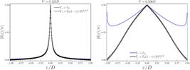
|δ(ε)/π| as function of the energy computed for V = 0.125D (left panel) and V = 0.500D (right panel). The black curves represent the numerical (circular dots) and analytical (solid line) results for the phase shift (equation (81)), while the blue solid line shows the phase shift obtained for a constant hybridization (equation (58)). The numerical data were obtained by brute-force diagonalization of the matrix representation of the model with 2L = 5000, Γ₀ = πρV² and ε_d = 0.

We also notice that the analytical results (black line) remain in an excellent agreement with the numerical data (circular dots). Small differences appear near the band edges, likely due to the instabilities of the numerical integration and/or finite sizes effects. These two examples of the NI-SIAM with non-trivial couplings and/or dispersions offer a general overview of the types of problems that the general solution presented here can address.

7. Conclusions

In this work, we provided a detailed and self-contained presentation of the application of the Sommerfeld-Watson transformation in the diagonalization procedure of two fundamental and significant Hamiltonians in condensed matter physics: the Fermi gas and the non-interacting single-impurity Anderson model (NI-SIAM). We also compared the analytical results with those obtained from brute-force numerical diagonalization of these models for different parameters, revealing excellent agreement between them.

Furthermore, we considered a more general NI-SIAM, in which no specific dispersion relation was assumed for the band energies, and the couplings in the Hamiltonian were allowed to vary depending on the band levels they couple to (controlled by the function α(ε)). Despite the increased mathematical complexity, we demonstrated that the same procedure used for the Fermi gas and the simpler NI-SIAM can successfully diagonalize this more general model. To the best of our knowledge, no previous work has derived the expression we obtained for this extended case.

In addition, we presented two non-trivial examples where our analytical solution can be applied: (i) an impurity coupled to a band through a semi-circular hybridization, and (ii) an effective mass band coupled to an impurity via finite-range hybridization. In both cases, the analytical results were compared with those obtained through numerical diagonalization, and the agreement between them was excellent.

Nevertheless, although the generalized NI-SIAM solution presented here can be applied to many different impurity-band systems, or to Fermi gases in the presence of non-trivial scattering potentials, it has its limitations.

The main one is that, while the generalized NI-SIAM Hamiltonian is flexible enough to include either a generic scattering potential or a generic hybridization individually, problems where both are represented by complex functions simultaneously may fall beyond the scope of the generalized solution presented here. The presented solution allows for only a single function α(ε) to controls the coupling amplitudes as a function of energy. Additionally, there are quadratic problems that cannot be diagonalized using this SWT-based procedure in its current form, or at least would require adaptations of the method presented here.

It is important to mention that the diagonalization procedure detailed in this work goes beyond the general NI-SIAM considered here. Future studies may apply this SWT-based method presented here to diagonalize different types of quadratic models.

In condensed matter physics, most problems begin by either diagonalizing a Hamiltonian or applying approximate methods, such as perturbation theory, to determine its eigenenergies and eigenvectors. Future research involving the diagonalization of impurity-band systems, or a band (or Fermi gas) in the presence of a scattering potential, may find this work a valuable reference. Such studies can benefit from the generalized NI-SIAM analytical solutions presented here, as well as from the detailed explanation of this non-perturbative diagonalization method.

Condensed matter physics professors can also rely on this work to explore the physics of these Fermi gas-like models in their classes, or to compare the solutions presented here (which are essentially exact in the large number of particles limit) with other methods, such as the Green’s function perturbative expansion, a common tool used to study these same problems within the scattering theory formalism. This makes the present work a valuable pedagogical tool for teaching the properties of these models.

Lastly, we want to emphasize that, despite their simplicity, these simple models discussed here have historically driven the discovery of important new phenomena, as previously discussed. Although analytical calculations rarely lead to entirely new physics these days, complex Hamiltonians can often be reduced to cases similar to those considered here, where analytical solutions are possible. Such simplifications, combined with the analytical diagonalization described here (or others analytical methods), can offer valuable insights into the underlying mechanisms governing more complex phenomena.

Acknowledgments

The authors would like to thank Prof. Dr. L. N. Oliveira for introducing and explaining this method to us for the first time. The authors would also like to acknowledge Prof. Dr. L. N. Oliveira for his supervision and all the knowledge he shared with us. G. Diniz acknowledges a PhD scholarship from the Brazilian agency Coordenação de Aperfeiçoamento de Pessoal de Nível Superior (CAPES – grant No. 88887.495890/2020-00). F. D. Picoli acknowledges PhD and internship fellowships from Fundação de Amparo à Pesquisa do Estado de São Paulo (FAPESP – grants 2022/09312-4 and 2024/05637-1). M. P. Lenzarini acknowledges funding from CAPES (Grant No. 88887.941429/2024-00).

Appendix A.

Finding the Commutators

Here, we aim to compute a general commutator that can be used to derive the main commutators presented in the text. In our notation, $[\widehat{A},\widehat{B}]$ denotes the commutator, while $\{\widehat{A},\widehat{B}\}$ represents the anti-commutator. Since we are dealing with fermionic operators ${\widehat{c}}_k^{†}$, they obey the relation $\{{\widehat{c}}_q,{\widehat{c}}_k^{†}\}={\delta }_{q,k}^K$, where ${\delta }_{q,k}^K$ is the Kronecker delta. This general commutator can be obtained following the above calculation:

(A1) $$\begin{array}{ll}\hfill & \left[{\displaystyle \sum _{q,q^{\prime }}{M}_{q,q^{\prime }}}{\widehat{c}}_q^{†}{\widehat{c}}_{q^{\prime }},{\widehat{c}}_k^{†}\right]\hfill \\ \hfill & ={\displaystyle \sum _{q,q^{\prime }}{M}_{q,q^{\prime }}}\left[{\widehat{c}}_q^{†}{\widehat{c}}_{q^{\prime }},{\widehat{c}}_k^{†}\right],\hfill \\ \hfill & ={\displaystyle \sum _{q,q^{\prime }}{M}_{q,q^{\prime }}}\left({\widehat{c}}_q^{†}{\widehat{c}}_{q^{\prime }}{\widehat{c}}_k^{†}-{\widehat{c}}_k^{†}{\widehat{c}}_q^{†}{\widehat{c}}_{q^{\prime }}\right),\hfill \\ \hfill & ={\displaystyle \sum _{q,q^{\prime }}{M}_{q,q^{\prime }}}\left({\widehat{c}}_q^{†}\left({\delta }_{k,q^{\prime }}^K-{\widehat{c}}_k^{†}{\widehat{c}}_{q^{\prime }}\right)-{\widehat{c}}_k^{†}{\widehat{c}}_q^{†}{\widehat{c}}_{q^{\prime }}\right),\hfill \\ \hfill & ={\displaystyle \sum _{q,q^{\prime }}{M}_{q,q^{\prime }}}\left({\widehat{c}}_q^{†}{\delta }_{k,q^{\prime }}^K-{\widehat{c}}_q^{†}{\widehat{c}}_k^{†}{\widehat{c}}_{q^{\prime }}-{\widehat{c}}_k^{†}{\widehat{c}}_q^{†}{\widehat{c}}_{q^{\prime }}\right),\hfill \\ \hfill & ={\displaystyle \sum _{q,q^{\prime }}{M}_{q,q^{\prime }}}\left({\widehat{c}}_q^{†}{\delta }_{k,q^{\prime }}^K-\left\{{\widehat{c}}_q^{†},{\widehat{c}}_k^{†}\right\}{\widehat{c}}_{q^{\prime }}\right),\hfill \\ \hfill & ={\displaystyle \sum _q{M}_{q,k}}{\widehat{c}}_q^{†}.\hfill \end{array}$$

This result, shown in equation (Appendix A) can be used to easily derive all commutators used in this work, one needs only to choose the coefficient M_q,q’ accordingly.

Appendix B.

Finding the Eigenvalue and Eigenoperators

Using the equality defined in equation (5) by substituting ${\widehat{g}}_m^{†}$ with the linear combination defined in equation (3) and after some algebraic manipulation, we find

(B1) $${\displaystyle \sum _k\left[{\epsilon }_k{u}_{k,m}+M_k{\displaystyle \sum _q{\overline{M}}_q}{u}_{q,m}+{\overline{M}}_k^{*}{\displaystyle \sum _q{M}_q^{*}}{u}_{q,m}\right]}{\widehat{c}}_k^{†}={\displaystyle \sum _k{ϵ}_m}{u}_{k,m}{\widehat{c}}_k^{†}.$$

As the operators ${\widehat{c}}_k^{†}$ are linearly independent, each term of the k-sum above has to satisfy the above equation independently,

(B2) $$u_{k,m}=\frac{M_k}{\left({ϵ}_m-{\epsilon }_k\right)}{\displaystyle \sum _q{\overline{M}}_q}{u}_{q,m}+\frac{{\overline{M}}_k^{*}}{\left({ϵ}_m-{\epsilon }_k\right)}{\displaystyle \sum _q{M}_q^{*}}{u}_{q,m}.$$

After multiplying both sides of equation (B2) by ${\overline{M}}_k$ summing over all k states, we find

(B3) $$\left[1-{\displaystyle \sum _k\frac{{\overline{M}}_k{M}_k}{{ϵ}_m-{\epsilon }_k}}\right]{\displaystyle \sum _q{\overline{M}}_q}{u}_{q,m}={\displaystyle \sum _k\frac{|{\overline{M}}_k{|}^2}{{ϵ}_m-{\epsilon }_k}}{\displaystyle \sum _k{M}_q^{*}}{u}_{q,m},$$

and now multiplying both sides of equation (B2) by $M_k^{*}$ summing over all k states, we find

(B4) $$\left[1-{\displaystyle \sum _k\frac{{\overline{M}}_k^{*}{M}_k^{*}}{{ϵ}_m-{\epsilon }_k}}\right]{\displaystyle \sum _q{M}_q^{*}}{u}_{q,m}={\displaystyle \sum _k\frac{|M_k{|}^2}{{ϵ}_m-{\epsilon }_k}}{\displaystyle \sum _k{\overline{M}}_q}{u}_{q,m}.$$

Considering that the terms $|{\sum }_q{M}_q^{*}{u}_{q,m}|$ and $|{\sum }_q{\overline{M}}_q{u}_{q,m}|$ are nonzero, the system of equations defined in equations (B3) and (B4) leads to

(B5) $${\left|1-{\displaystyle \sum _k\frac{{\overline{M}}_k{M}_k}{{ϵ}_m-{\epsilon }_k}}\right|}^2={\displaystyle \sum _k\frac{|M_k{|}^2}{{ϵ}_m-{\epsilon }_k}}{\displaystyle \sum _k\frac{|{\overline{M}}_k{|}^2}{{ϵ}_m-{\epsilon }_k}}.$$

The equation defined in equation (B5) represents the eigenvalue equation, and the set of values {ϵ_m} that satisfy this equation are the eigenvalues of the Hamiltonian. This is precisely where the Sommerfeld-Watson transformation becomes highly useful, as it allows us to find functions that simplify the summations

(B6) $$\begin{array}{c}S(ϵ)={\displaystyle \sum _k\frac{|M_k{|}^2}{ϵ-{\epsilon }_k}},\overline{S}(ϵ)={\displaystyle \sum _k\frac{|{\overline{M}}_k{|}^2}{ϵ-{\epsilon }_k}},\text{and}\\ \tilde{S}(ϵ)={\displaystyle \sum _k\frac{M_k{\overline{M}}_k}{ϵ-{\epsilon }_k}},\end{array}$$

and the solutions to the equation ${\left|1-\tilde{S}(ϵ)\right|}^2=S(ϵ)\tilde{S}(ϵ)$ give us the eigenvalues of $\widehat{H}$.

Manipulating equation (B2) and imposing the normalization condition ∑_k|u_k,m|² = 1, it is straightforward to show that

(B7) $$\begin{array}{ll}1=\hfill & -\frac{\text{d}S(ϵ)}{}{\left|{\displaystyle \sum _q{\overline{M}}_q}{u}_{q,m}\right|}^2-\frac{\text{d}\overline{S}(ϵ)}{\text{d}ϵ}{\left|{\displaystyle \sum _q{M}_q^{*}}{u}_{q,m}\right|}^2\hfill \\ \hfill & -2\text{Re}\left(\frac{\text{d}\tilde{S}(ϵ)}{\text{d}ϵ}{\displaystyle \sum _q{M}_q}{u}_{q,m}{\displaystyle \sum _q{\overline{M}}_q}{u}_{q,m}\right).\hfill \end{array}$$

Finding these summations over k enables us to determine the terms ${\sum }_q{\overline{M}}_q{u}_{q,m}$ and ${\sum }_q{M}_q^{*}{u}_{q,m}$, which in turn allows us to calculate u_q,m, thereby completing the diagonalization procedure.

Appendix C.

A more general solution

We can write the Hamiltonian in equation (69) compactly as

(C1) $$\widehat{H}={\displaystyle \sum _{\kappa }{\epsilon }_{\kappa }}{\widehat{c}}_{\kappa }^{†}{\widehat{c}}_{\kappa }+{\displaystyle \sum _{\kappa ,\xi }\left(M_{\kappa }{\overline{M}}_{\xi }+M_{\xi }^{*}{\overline{M}}_{\kappa }^{*}\right)}{\widehat{c}}_{\kappa }^{†}{\widehat{c}}_{\xi }.$$

Here, the index κ runs over the impurity level d and band levels k, the index ξ runs over d and band levels q, and the coupling can be expressed as

(C2) $$\begin{array}{ll}{M}_{\kappa }\hfill & =\sqrt{\frac{W}{4L}}(1-{\delta }_{\kappa ,d}^K){\alpha }_k^{*}\text{and}{\overline{M}}_{\xi }\hfill \\ \hfill & =\frac{V}{\sqrt{W/2}}{\delta }_{\xi ,d}^K+\sqrt{\frac{W}{4L}}(1-{\delta }_{\xi ,d}^K){\alpha }_q,\hfill \end{array}$$

where ${\delta }_{\kappa ,\xi }^K$ stands for the Kronecker’s delta.

C.1. The general phase shift

The compact Hamiltonian in equation (C1) allows us to directly use all equations deduced in the previous appendix, particularly the eigenvalue equation in (6). Using the couplings defined by equation (C2) leads to:

(C3) $$\begin{array}{lll}S(ϵ)\hfill & =\hfill & {\displaystyle \sum _k\frac{|M_k{|}^2}{ϵ-{\epsilon }_k}}=\frac{W}{4L}{\displaystyle \sum _k\frac{|{\alpha }_k{|}^2}{ϵ-{\epsilon }_k}},\hfill \\ \overline{S}(ϵ)\hfill & =\hfill & {\displaystyle \sum _k\frac{|{\overline{M}}_k{|}^2}{ϵ-{\epsilon }_k}}=\frac{2V^2/W}{ϵ-{\epsilon }_d}+S(ϵ),\hfill \\ \tilde{S}(ϵ)\hfill & =\hfill & {\displaystyle \sum _k\frac{M_k{\overline{M}}_k}{ϵ-{\epsilon }_k}}=S(ϵ)\hfill \end{array}$$

and

(C4) $${\left|1-\frac{W}{4L}{\displaystyle \sum _k\frac{|{\alpha }_k{|}^2}{ϵ-{\epsilon }_k}}\right|}^2=\left[\frac{2V^2/W}{ϵ-{\epsilon }_d}+\frac{W}{4L}{\displaystyle \sum _k\frac{|{\alpha }_k{|}^2}{ϵ-{\epsilon }_k}}\right]\frac{W}{4L}{\displaystyle \sum _k\frac{|{\alpha }_k{|}^2}{ϵ-{\epsilon }_k}}.$$

A more convenient notation is obtained by substituting |α_k|² by w_k.

We observe that the term $S_0(ϵ)=\frac{1}{2L}{\sum }_k\frac{w_k}{ϵ-{\epsilon }_k}$ appears repeatedly in the equations above. Thus, our solution relies on evaluating this summation. To proceed after this point, some assumptions are necessary. First, we will assume that w_k can be expressed as a continuous function w(k) and it does not have poles. The Sommerfeld-Watson transformation then allowed us to express the summation as

(C5) $$S_0(ϵ)=\frac{1}{2L}{\displaystyle \sum _k\frac{w_k}{ϵ-{\epsilon }_k}}=\frac{1}{2i}{\displaystyle \oint \frac{dz}{2L}}\frac{w(z)\cot (\pi z)}{ϵ-{\epsilon }_z}$$

(C6) $$-\frac{\pi }{2L}{\displaystyle \sum _{p}w(z_p(ϵ))}\cot (\pi z_p(ϵ))\text{Res}{\left(\frac{1}{ϵ-{\epsilon }_z}\right)}_{z=z_p},$$

or

(C7) $$\begin{array}{ll}{S}_0(ϵ)=\hfill & \frac{1}{2i}{\displaystyle \oint \frac{dz}{2L}}\frac{w(z)\cot (\pi z)}{ϵ-{\epsilon }_z}\hfill \\ \hfill & -\frac{\pi }{2L}{\displaystyle \sum _{p}w}(z_p(ϵ))\cot (\pi z_p(ϵ))\text{Res}{\left(\text{}\frac{1}{ϵ-{\epsilon }_z}\text{}\right)}_{z=z_p}\text{}\text{}.\hfill \end{array}$$

Here, z_p(ϵ) represents the poles of (ϵ − ε_z)⁻¹, that is ε_zp = ϵ. Let us recall that the variable z is a continuous complex extension of the discrete variable k, which labels the band level ε_k.

For simplicity, let us consider a non-degenerate pole, that is, a single value of z_p. This step can also be applied to a degenerate spectrum. However, in most cases, a degenerate spectrum is lifted in the presence of a perturbation. In the rare situations where the degeneracy remains relevant even in the presence of the perturbation, it is necessary to adapt this step to account for this effect, usually by defining an additional degeneracy function to incorporate it.

After the above considerations, by using the same complex counter defined in Fig. 2 and the density of states defined in equation (70) with no poles near the energy ϵ, it is straightforward to show that

(C8) $$\begin{array}{ll}{S}_0(ϵ)=\hfill & 𝒫{\displaystyle {\int }_{-D}^{+D}d\epsilon }\frac{\rho (\epsilon )w_{\epsilon }}{ϵ-\epsilon }-\pi \rho (ϵ)w(ϵ)\cot (\pi z(ϵ))\hfill \\ \hfill & \cdot \text{Res}{\left(\frac{1}{2L\rho (ϵ)}\frac{1}{ϵ-{\epsilon }_z}\right)}_{{\epsilon }_z=ϵ}.\hfill \end{array}$$

A general energy dispersion can be expressed as ε_z = ε(0) + γ ⋅ z^β, where γ and β are constants. Then, from equation (70), the density of states is given by $\rho ({\epsilon }_z)=\frac{1}{2L}{\left(\gamma \beta z^{\beta -1}\right)}^{-1}$. With this in mind, let us compute the following limit

(C9) $$\begin{array}{ll}\underset{z\to z(ϵ)}{\lim }\frac{1}{2L\rho ({\epsilon }_z)}\frac{z-z(ϵ)}{{\epsilon }_z-ϵ}\hfill & =\underset{z\to z(ϵ)}{\lim }\frac{1}{2L\rho ({\epsilon }_z)}\frac{z-z(ϵ)}{\gamma \cdot z^{\beta }-ϵ}\hfill \\ \hfill & =\underset{z\to z(ϵ)}{\lim }\frac{1}{2L\rho ({\epsilon }_z)}{\left(\gamma \beta k^{\beta -1}\right)}^{-1}\hfill \\ \hfill & =1.\hfill \end{array}$$

Clearly, the pole is simple around the energy ϵ, and the residue can be computed by the above expression, resulting in

(C10) $$\text{Res}{\left(\frac{1}{2L\rho (ϵ)}\frac{1}{ϵ-{\epsilon }_z}\right)}_{{\epsilon }_z=ϵ}=-1,$$

and

(C11) $$S_0(ϵ)=𝒫{\displaystyle {\int }_{-D}^{+D}d\epsilon }\frac{\rho (\epsilon )w_{\epsilon }}{ϵ-\epsilon }+\pi \rho (ϵ)w(ϵ)\cot (\pi z(ϵ)).$$

Finally, once the pole ϵ−ε_k results in a z(ϵ) near z = k, we can write z(ϵ) = k − δ(ϵ)/π, and our expression for the summation becomes:

(C12) $$S_0(ϵ)=𝒫{\displaystyle {\int }_{-D}^{+D}d\epsilon }\frac{\rho (\epsilon )w_{\epsilon }}{ϵ-\epsilon }-\pi \rho (ϵ)w(ϵ)\cot (\delta (ϵ)).$$

Now, let us split the function S₀(ϵ) = 𝒮(ϵ) + ρ(ϵ)w(ϵ)ℐ(ϵ) by defining

(C13) $$ℐ(ϵ)=\frac{1}{\rho (ϵ)w(ϵ)}𝒫{\displaystyle {\int }_{-D}^{+D}d\epsilon }\frac{\rho (\epsilon )w_{\epsilon }}{ϵ-\epsilon },$$

and

(C14) $$𝒮(ϵ)=\pi \rho (ϵ)w(ϵ)\cot (\pi z(ϵ)).$$

Now, returning to equation (C4), we can write

(C15) $$\begin{array}{l}1-W\left(𝒮(ϵ)+\rho (ϵ)w(ϵ)ℐ(ϵ)\right)\\ =\frac{V^2}{ϵ-{\epsilon }_d}\left(𝒮(ϵ)+\rho (ϵ)w(ϵ)ℐ(ϵ)\right),\end{array}$$

resulting in the expression

(C16) $$𝒮(ϵ)\left(\frac{V^2}{ϵ-{\epsilon }_d}+W\right)=1-\rho (ϵ)w(ϵ)\left(\frac{V^2}{ϵ-{\epsilon }_d}+W\right)ℐ(ϵ).$$

Finally, once the pole ϵ−ε_k results in a z(ϵ) near z = k, we can write z(ϵ) = k − δ(ϵ)/π, and our expression for the phase shift becomes

(C17) $$\tan \delta (ϵ)=\tan {\delta }^{(0)}(ϵ){\left(1+\frac{\tan {\delta }^{(0)}(ϵ)}{\pi }ℐ(ϵ)\right)}^{-1}.$$

where

(C18) $$\tan {\delta }^{(0)}(ϵ)=-\pi w(ϵ)\rho (ϵ)W-\frac{\text{Γ}(ϵ)}{ϵ-{\epsilon }_d}.$$

Here, the hybridization function is defined as Γ(ϵ) = πw(ϵ)ρ(ϵ)V².

C.2. The general coefficients

As shown in Appendix B, the coefficients can be determined using the auxiliary equation (B7). As observed in equation (C.1), all the key summations can be obtained by computing S₀. Consequently, to extract information from equation (B7), we first need to compute its derivative in the following expression

(C19) $$-\frac{1}{2L}\frac{\text{d}{S}_0(ϵ)}{\text{d}ϵ}=\frac{{\pi }^2{\rho }^2(ϵ)w(ϵ)}{{\sin }^2(\delta (ϵ))}+\frac{\pi }{2L}\cot (\delta (ϵ))\frac{\text{d}}{\text{d}ϵ}\left(\rho (ϵ)w(ϵ)\right)\text{}\text{}-\frac{1}{2L}\frac{\text{d}}{\text{d}ϵ}\left(𝒫{\displaystyle {\int }_{-D}^{+D}dϵ}\frac{\rho (\epsilon )w_{\epsilon }}{ϵ-\epsilon }\right).$$

Here, the fraction 1/2L was inserted to show how much larger the first term on the left side of the above equation is compared to the other terms. As a result, we can drop these lesser contributions, resulting in

(C20) $$-\frac{1}{2L}\frac{\text{d}{S}_0(ϵ)}{\text{d}ϵ}={\pi }^2{\rho }^2(ϵ){\sin }^{-2}(\delta (ϵ))w(ϵ)+𝒪\left({(2L)}^{-1}\right).$$

For simplicity, let us define $x_1={\sum }_q{\overline{M}}_q{u}_{q,m}$ and $x_2={\sum }_q{M}_q^{*}{u}_{q,m}$, transforming the system of equations formed by equations (B4) and (B7) into

(C21) $$\left[1-S(ϵ)\right]x_2=S(ϵ)x_1,$$

and

(C22) $$1=-\frac{\text{d}S(ϵ)}{\text{d}ϵ}{x}_1^2+\left[\frac{2V^2/W}{{(ϵ-{\epsilon }_d)}^2}-\frac{\text{d}S(ϵ)}{\text{d}ϵ}ϵ\right]x_2^2-2\frac{\text{d}S(ϵ)}{\text{d}ϵ}{x}_1{x}_2,$$

respectively. After grouping the common terms $\frac{\text{d}S}{\text{d}ϵ}$ of the above equation, we obtain

(C23) $$1=-\frac{\text{d}S(ϵ)}{\text{d}ϵ}{\left(x_1+x_2\right)}^2+\left[\frac{2V^2/W}{{(ϵ-{\epsilon }_d)}^2}\right]x_2^2.$$

Now, we only need a relation between x₁ and x₂ to finally find them.

Keeping that in mind, isolating x₂ from equation (C21) and substituting into equation (C23) results in the following expression

(C24) $$1=\left[-\frac{dS(ϵ)}{dϵ}+\frac{2V^2/W}{{(ϵ-{\epsilon }_d)}^2}{S}^2(ϵ)\right]{(x_1+x_2)}^2.$$

Now, by substituting $S(ϵ)=\frac{W}{2}{S}_0$ and using the result found in equation (C20), it is straightforward to show that

(C25) $$1={\left[\sqrt{\frac{2LW}{2}}\frac{\pi \rho (ϵ)}{\sin (\delta (ϵ))}\sqrt{w(ϵ)}\right]}^2\cdot \left(1+𝒪\left({(2L)}^{-2}\right)\right){(x_1+x_2)}^2,$$

and consequently the expression

(C26) $$(x_1+x_2)\approx {\left[\sqrt{\frac{2LW}{2}}\frac{\pi \rho (ϵ)}{\sin (\delta (ϵ))}\sqrt{w(ϵ)}\right]}^{-1}.$$

A combination of equation (B2) with the general couplings defined in equation (C2) results in the following expression

(C27) $$u_{k,m}=\sqrt{\frac{Ww({\epsilon }_k)}{4L}}\frac{{(x_1+x_2)}_{ϵ={ϵ}_m}}{\left({ϵ}_m-{\epsilon }_k\right)},$$

which depends exactly on the quantity x₁ + x₂ already found.

Continuing the calculations, the general coefficients can be obtained by substituting equation (C26) into equation (C27), resulting in

(C28) $$u_{k,m}\approx -\frac{1}{2L}\frac{\sqrt{w({\epsilon }_k)}}{\sqrt{w({ϵ}_m)}}\frac{\sin (\delta ({ϵ}_m))}{\pi \rho ({ϵ}_m)}\frac{1}{{ϵ}_m-{\epsilon }_k}.$$

Finally, by defining the quantity

(C29) $${\text{Δ}}_{k,m}=\frac{1}{2L\rho ({\epsilon }_m)}\sqrt{\frac{w({\epsilon }_k)}{w({\epsilon }_m)}},$$

the expression for the coefficients can be written in the familiar form as

(C30) $$u_{k,m}\approx -\frac{\sin ({\delta }_m)}{\pi }\frac{{\text{Δ}}_{k,m}}{{ϵ}_m-{\epsilon }_k}.$$

Completing the diagonalization procedure for this more general Hamiltonian.

Data Availability

All data generated in this work, numerical diagonalization codes in the Julia language, and Python codes used for the plots are available at: https://doi.org/10.7910/DVN/R12Y7X.

References

• ^[1] A. Sommerfeld, Partial differential equations in physics (Academic Press, London, 1949).
• ^[2] J. Mathews and R.L. Walker, Mathematical Methods of Physics (Benjamin, Menlo Park, 1970).
• ^[3] M.L. Rumerman, The Journal of the Acoustical Society of America 91, 2502 (1992).
• ^[4] M.M. Islam, Nuclear Physics B 104, 511 (1976).
• ^[5] M.K. Li and W.C. Chew, IEEE Antennas and Wireless Propagation Letters 3, 75 (2004).
• ^[6] W. Drechsler, Il Nuovo Cimento A 61, 1 (1969).
• ^[7] P. Goddard and A.R. White, Nuovo Cimento A 1, 645 (1971).
• ^[8] N.N. Khuri, Physical Review Letters 10, 420 (1963).
• ^[9] J.B. Hartle, Physical Review 134, B612 (1964).
• ^[10] J.S. Frederiksen, Communications in Mathematical Physics 43, 1 (1975).
• ^[11] J. Pumplin, American Journal of Physics 37, 737 (1969).
• ^[12] C.A. Valagiannopoulos, Progress In Electromagnetics Research 75, 137 (2007).
• ^[13] C.A. Valagiannopoulos, Progress In Electromagnetics Research 71, 277 (2007).
• ^[14] S. Sen and M. Kuzuoglu, Progress In Electromagnetics Research 84, 55 (2008).
• ^[15] P.W. Anderson, Physical Review 124, 41 (1961).
• ^[16] G.D. Mahan, Many-Particle Physics, Physics of Solids and Liquids (Springer, New York, 2010).
• ^[17] G.D. Mahan, Physical Review 163, 612 (1967).
• ^[18] P. Nozières and C.T. De Dominicis, Physical Review 178, 1097 (1969).
• ^[19] M. Combescot and P. Nozières, Journal De Physique 32, 913 (1971).
• ^[20] L.N. Oliveira and J.W. Wilkins, Physical Review B 24, 4863 (1981).
• ^[21] L.N. Oliveira and J.W. Wilkins, Physical Review B 32, 696 (1985).
• ^[22] S. Doniach and M. Sunjic, Journal of Physics C 3, 285 (1970).
• ^[23] K. Ohtaka and Y. Tanabe, Reviews of Modern Physics 62, 929 (1990).
• ^[24] G. Diniz, Sticking coefficient for atoms impinging on a metallic surfaces, and the x-ray photoemission by metals Doctoral Thesis, University of São Paulo, São Carlos (2024).
• ^[25] V.L. Libero and L.N. Oliveira, Physical Review B 42, 3167 (1990).
• ^[26] F.D. Picoli, G. Diniz, M.P. Lenzarini, I. D’Amico and L.N. Oliveira, arXiv:2502.11317 (2025).
• ^[27] G. Diniz, F.D. Picoli, L.N. Oliveira and I. D’Amico, arXiv:2502.11313 (2025).
• ^[28] W.C. Oliveira and L.N. Oliveira, Physical Review B 49, 11986 (1994).
• ^[29] A.L. Ferrari and L.N. Oliveira, Physical Review B 106, 075129 (2022).
• ^[30] P. Nozières, Journal of Low Temperature Physics 17, 31 (1974).
• ^[31] M.A. Kastner, Reviews of Modern Physics 64, 849 (1992).
• ^[32] K.G. Wilson, Reviews of Modern Physics 47, 773 (1975).
• ^[33] P.W. Anderson, Physical Review Letters 18, 1049 (1967).
• ^[34] E. Butkov, Mathematical Physics (Addison-Wesley, Reading, 1973).
• ^[35] M.G. Rozman, Summation of series: Sommerfeld-Watson transformation, available in: https://www.ph ys.uconn.edu/~rozman/Courses/P2400_16S/downloa ds/sommerfeld-watson.pdf, accessed on 24/06/2025.
  » https://www.ph ys.uconn.edu/~rozman/Courses/P2400_16S/downloa ds/sommerfeld-watson.pdf
• ^[36] G. Greczynski and L. Hultman, Progress in Materials Science 107, 100591 (2020).
• ^[37] C.T. Chantler, G. Bunker, P. D’Angelo and S. Diaz Moreno, Nature Reviews Methods Primers 4, 89 (2024).
• ^[38] J.J. Sakurai and Jim Napolitano, Modern quantum mechanics (Cambridge University Press, Cambridge, 2020), 3 ed.
• ^[39] G. Diniz, G.S. Diniz, G.B. Martins and E. Vernek, Physical Review B 101, 125115 (2020).
• ^[40] P. Schlottmann, Zeitschrift für Physik B Condensed Matter 51, 223 (1983).
• ^[41] R. Bulla, T.A. Costi and T. Pruschke, Reviews of Modern Physics 80, 395 (2008).
• ^[42] S.R. White and A.E. Feiguin, Physical Review Letters 93, 076401 (2004).
• ^[43] S.R. White, Physical Review Letters 69, 2863 (1992).
• ^[44] D.M. Newns, Physical Review 178, 1123 (1969).
• ^[45] N.W. Ashcroft and N.D. Mermin, Solid State Physics (Holt, Rinehart and Winston, Michigan, 1976).
• ^[46] L. Van Hove, Physical Review 89, 1189 (1953).
• ^[47] A. Gerges, G. Kotliar, W. Krauth and M.J. Rozenberg, Reviews of Modern Physics 68, 13 (1996).

• 1
  For mostly problems, it is possible, without loss of generality, to simplify the procedure by assuming that the coefficients {u_k,m} are real numbers.
• 2
  It is assumed that the reader is already familiar with complex analysis; if not, it is recommended to first consult Mathematical Physics by Eugene Butkov.
• 3
  The fraction $\frac{\cot (\pi z)}{z^2+{\eta }^2}$ goes to zero at all points of the contour in the |z| → ∞ limit.
• 4
  We used the Julia programming language to diagonalize the matrix representation of the Hamiltonian. However, this straightforward diagonalization can be carried out in any programming language.
• 5
  Note the singularity around zero energy in equation (79). Moreover, the same analysis applied to the phase shift can be directly translated to the coefficients, as previously discussed.
• 6
  In the simplest case of the Hubbard model, all sites have the same energy. Therefore, by translational symmetry, the impurity energy must be fixed at zero.

Edited by

• Editor-in-Chief:
  Marcello Ferreira https://orcid.org/0000-0003-4945-3169

Publication Dates

• Publication in this collection
  01 Aug 2025
• Date of issue
  2025

History

• Received
  28 Mar 2025
• Reviewed
  23 May 2025
• Accepted
  13 June 2025