
 ARIMA modeling for predicting hair coat temperature in dairy cows under heat stress1
ABSTRACT
Hair coat temperature is an effective indicator for monitoring heat stress in dairy cows, particularly in tropical regions, as it directly reflects environmental conditions and animal adaptation. Autoregressive Integrated Moving Average models with transfer functions enable dynamic assessment of the relationship between environmental variables and physiological responses. This study evaluated the influence of the temperature-humidity index and ambient temperature on hair coat temperature, as well as its temporal response to heat stress, considering differences related to age and parity. Hair coat temperature was measured at the head, back, udder, and cannon bone of 19 Holstein cows housed in a free-stall system, twice daily over 229 days. The model was fitted to the input series to predict the output series (hair coat temperature). Seasonal conditions significantly affected hair coat temperature, and cross-correlation analysis indicated a rapid thermal response to heat stress with short-term persistence, generally between 24 and 48 hours. Ambient temperature showed a significant causal relationship with hair coat temperature, and the transfer function model demonstrated good predictive performance (Root Mean Square Error = 1.08 °C). Younger cows and those with lower parity were more thermally vulnerable, whereas adult, multiparous cows showed greater thermal stability. Predictive modeling proved to be a promising tool for studying the thermal dynamics of Holstein cows. However, the results are limited to this breed and the local climatic conditions and should not be extrapolated to other production contexts.
Key words:
transfer function; seasons; cross-correlation; lagged response; free stall
HIGHLIGHTS:
ARIMA models accurately predict hair coat temperature in Holstein cows under intense heat stress conditions.
Seasonal factors, such as ambient temperature and the temperature-humidity index, influence bovine coat temperature.
Younger and primiparous cows are more susceptible to heat stress than multiparous cows.
RESUMO
A temperatura do pelame é um indicador eficiente para o monitoramento do estresse térmico em vacas leiteiras, especialmente em regiões tropicais, pois reflete diretamente as condições climáticas e a adaptação dos animais. Modelos de média móvel integrada autorregressiva (ARIMA) com funções de transferência permitem avaliar, de forma dinâmica, a relação entre variáveis ambientais e respostas fisiológicas. Este estudo avaliou a influência do índice de temperatura e umidade e da temperatura ambiente sobre a temperatura do pelame, bem como sua resposta temporal ao estresse térmico, considerando diferenças relacionadas à idade e à paridade. A temperatura do pelame foi mensurada na cabeça, dorso, úbere e canela de 19 vacas da raça Holandesa, mantidas em sistema de baias livres, duas vezes ao dia, durante 229 dias. O modelo foi ajustado às séries de entrada para prever a série de saída (temperatura do pelame). As condições sazonais influenciaram significativamente a temperatura do pelame, e a análise de correlação cruzada indicou uma resposta térmica rápida ao estresse, com persistência de curto prazo, geralmente entre 24 e 48 horas. A temperatura ambiente apresentou relação causal significativa com a temperatura do pelame, e o modelo de função de transferência demonstrou bom desempenho preditivo (Erro Quadrático Médio = 1,08 °C). Vacas mais jovens e com menor paridade mostraram maior vulnerabilidade térmica, enquanto vacas adultas e multíparas apresentaram maior estabilidade. A modelagem preditiva mostrou-se uma ferramenta promissora para o estudo da dinâmica térmica de vacas Holandesas. Contudo, os resultados são restritos a essa raça e às condições climáticas locais, não devendo ser extrapolados para outros contextos produtivos.
Palavras-chave:
função de transferência; estações; correlação cruzada; resposta de atraso; baia livre
INTRODUCTION
Heat stress in dairy cows is one of the major challenges faced by producers in tropical and subtropical regions, such as South America (Almeida et al., 2010). Environmental conditions exceeding the thermo-neutral zone (5.0-25.0 °C), within which animals maintain normal physiological function, negatively affect dairy production (Daltro et al., 2020), leading to reductions in milk yield of up to 30%, particularly in Holstein cows (Liu et al., 2019).
The capacity of dairy cows to dissipate excess heat is limited, especially in breeds of European origin, such as Holsteins, due to low evaporative efficiency and high metabolic heat production (Li et al., 2021). As a result, heat stress is associated with increased body temperature and respiratory rate, along with reduced feed intake, ultimately causing substantial economic losses in dairy farming (Pacheco et al., 2020). Global annual losses attributable to heat stress in the dairy sector are estimated to exceed US$1.5 billion (Liu et al., 2019).
Among the indicators commonly used to monitor heat stress in dairy cows, coat temperature (CT) stands out for its sensitivity in reflecting the animal’s thermal balance and for the ease of assessment using noninvasive techniques such as infrared thermography (Pacheco et al., 2020; Shu et al., 2021). CT directly represents surface thermal conditions and the efficiency of heat dissipation, and has been shown to be more consistent than other physiological indicators under varying environmental conditions (Almeida et al., 2010).
Physiological responses of Holstein cows to heat stress are not instantaneous and may require 24-48 hours to stabilize following exposure (Li et al., 2021). These responses tend to be more pronounced in primiparous and secundiparous cows, which have additional energy demands for growth. This highlights the importance of evaluating the effects of age and parity on heat stress responses. Such dynamics emphasize the need to model the relationships between climatic variables, such as ambient temperature (TA) and the temperature-humidity index (THI), and CT, considering delayed or lagged responses (Dado-Senn et al., 2020; Li et al., 2021).
Holstein cows were selected for this study because they represent the predominant genotype in intensive dairy production systems and are widely used as a reference model in heat stress research. Their high milk yield is associated with elevated metabolic activity, resulting in greater endogenous heat production and increased sensitivity to adverse environmental conditions. Previous studies have shown that Holstein cows respond to heat stress with increases in body and surface temperatures and respiratory rate, accompanied by declines in productive performance (Liu et al., 2019; Becker et al., 2020). Importantly, these responses occur dynamically and with measurable time lags, reinforcing the suitability of time-series-based approaches for evaluating heat stress in this breed (Li et al., 2021). The use of Holstein cows therefore enhances the biological coherence of the findings and avoids inappropriate extrapolation to breeds with different adaptive and thermoregulatory capacities.
The objective of this study was to evaluate the influence of seasonal climatic conditions, represented by THI and TA, on CT in Holstein dairy cows, with emphasis on lagged responses and system dynamics under heat stress. The underlying hypothesis was that Autoregressive Integrated Moving Average (ARIMA) modeling with transfer functions represents an efficient, reliable approach for predicting lagged physiological responses with high accuracy. In addition, this study explored the application of ARIMA-based methods, including cross-correlation analysis and transfer function modeling, to predict CT and support more effective heat stress management in Holstein cows housed in free-stall confinement systems.
MATERIAL AND METHODS
All experimental procedures were approved by the Animal Use Ethics Committee (CEUA) at Instituto Federal de Educação, Ciência e Tecnologia do Sul de Minas (IFSULDEMINAS), Muzambinho campus, under protocol No. 3963040523 (MG, Brazil).
Data were collected from 19 Holstein cows with a mean of 45 ± 12.5 days in milk and a minimum daily milk yield of 15 ± 2.3 kg. Animals were housed in a free-stall facility measuring 54 m in length, 14 m in width, and 6 m in height, with capacity for up to 60 cows. Individual stalls measured 2.8 m in length and 1.3 m in width. The facility was equipped with natural daylight and artificial lighting at night, as well as a mixed ventilation system combining natural airflow with fans and air sprayers. These cooling devices were automatically activated when ambient temperature exceeded 23.0 °C and operated from 10 to 16 hours. The cows were fed a diet based on corn silage and a concentrate containing 25% crude protein, and received pre-filtered, chlorinated water ad libitum. The facility belongs to the Dairy Cattle Sector of the IFSULDEMINAS School Farm, Muzambinho campus (21° 20′ 28″ S, 46° 32′ 04″ W; and altitude of 1,034 m).
The cows were mechanically milked twice daily, in the morning and afternoon, using a fishbone-type milking parlor equipped with a Gea® low-line double-six system. During each milking session, temperatures of the head, back, cannon bone, and udder were measured using a portable digital thermometer (TI-550, Instrutherm) with valid calibration (No. 143482R/23, Instrutherm Calibration Laboratory). Coat temperature was calculated according to Eq. 1 (Almeida et al., 2010):
Where:
CT - coat temperature, in ºC;
HT - head temperature, in ºC;
DT - dorsal temperature, in ºC;
ST - shin temperature, in ºC; and,
UT - udder temperature, in ºC.
Temperature measurements were obtained during morning (7:00-8:00 hours) and afternoon (17:00-18:00 hours) milking sessions over 229 consecutive days, from August 2023 to March 2024, encompassing winter, spring, and summer seasons. In total, 34,808 records were collected, considering two daily milking sessions and four anatomical regions per cow. During milking, air sprayers were turned off to avoid interference with temperature measurements. Cows presenting clinical conditions were temporarily removed for treatment, and only clinically healthy animals were included in the dataset. Recorded variables included coat temperature, age, and parity. Mean coat temperature was 33.3 ± 1.4 °C, ranging from 27.3 to 35.7 °C. Mean parity was 2 ± 1.3 calvings (range: 1-6), and mean age was 4.5 ± 1.8 years (range: 2-9 years).
Meteorological data, including ambient temperature (°C) and relative air humidity (%), were recorded at 10-minute intervals using a calibrated datalogger (HT-900, Instrutherm; calibration No. 143488/23). The sensor was mounted on a tripod at a height of 1.20 m above ground level and operated continuously throughout the study. The temperature-humidity index was calculated using Eq. 2 (Liu et al., 2019):
Where:
THI - temperature-humidity index;
TA - ambient temperature, in ºC; and,
RH - relative air humidity, in %.
CT was defined as the output time series (OTS). The input time series (ITS) consisted of temperature-humidity index and ambient temperature. Each input was further subdivided into three series: maximum THI (THI_Max), average THI (THI_Med), minimum THI (THI_Min), maximum TA (TA_Max; ºC), average TA (TA_Med; ºC), and minimum TA (TA_Min; ºC).
ARIMA modeling is a time-series forecasting approach that combines autoregressive and moving average components to accommodate non-stationary data. In this study, autoregressive integrated moving average modeling with a transfer function was applied following methodological frameworks described by Li et al. (2021) and Khikmah et al. (2023), which guided parameter identification and model development.
ARIMA models are defined by the parameters (p, d, q), where p represents the autoregressive (AR) order, d indicates the number of differencing operations required to achieve stationarity, and q corresponds to the order of the moving average (MA) terms (Eq. 3).
Where:
ϕp(B) - AR process described by ϕp(B) = (1 - ϕ1B1 - ϕ2B2 - … - ϕpBp);
θq(B) - MA process described by θq(B) = (1 + θ1B1 + θ2B2 + … - θqBq); and,
et - it is the residual error.
The TF was used to make predictions of the OTS (Yt), defined based on the values of the ITS (Xt) (Eq. 4). Before its application, it was necessary to remove the pattern from the ITS (white noise). The same equation was then transferred and applied to the OTS (Eqs. 5 and 6).
Where:
Yt - output time series;
ωs(B) - numerator polynomial of the transfer function, defined as ωs(B) = ω0 - ω1B1 - ω2B2 - … - ωsBs;
δr(B) - denominator polynomial of the transfer function, defined as δr(B) = δ0 + δ1B1 + δ2B2 + … - δrBr;
B - backshift (lag) operator;
Xt-b - input time series with delay;
b - delay parameter indicating the initial lag at which the input series affects the output series;
θq(B) - moving average polynomial of order q associated with the noise component;
ϕp(B) - autoregressive polynomial of order p associated with the noise component;
at - random error term (white noise);
αt - pre-whitened input time series (ITS);
ϕx(B) - autoregressive polynomial used in the pre-whitening of the input time series;
θx(B) - moving average polynomial used in the pre-whitening of the input time series;
Xt - input time series;
βt - pre-whitened output time series (OTS);
ϕy(B) - autoregressive polynomial used in the pre-whitening of the output time series; and,
θy(B) - moving average polynomial used in the pre-whitening of the output time series.
The cross-correlation function (CCF) was used to evaluate the presence of correlations between αt and βt (post-whitening of the series) (Eqs.7 and 8). After this evaluation, the impulse response was calculated (Eq. 9) (Box et al., 2015) to determine the orders (r, s, b), which were subsequently used to construct the transfer function model (Eq. 4).
Where:
rxy (k) - cross-correlation coefficient between the time series X and Y at lag k;
k - lag of the cross-correlation function, with k=0,±1,±2,…;
- estimated cross-correlation coefficient between the time series X and Y;
cxy (k) - cross-covariance between the time series X and Y at lag k;
Sx - standard deviation of the time series X;
Sy - standard deviation of the time series Y;
n - sample size (number of observations);
t - time index;
Xt - value of the input time series X at time t;
X - mean of the input time series X;
Yt+k - value of the output time series Y at time t+k;
Y - mean of the output time series Y;
vk - impulse response at lag k;
rαβ (k) - cross-correlation function between the pre-whitened input series αt and the pre-whitened output series βt;
Sα - standard deviation of the pre-whitened output time series; and,
Sβ - standard deviation of the pre-whitened input time series.
In the ARIMA model based on the transfer function (TF), the orders (r, s, b) define the relationship between the ITS (Xt) and the OTS (Yt). In this context: r represents the number of lags of Xt that affect Yt; s indicates the number of lags of Yt; and b is the initial lag at which Xt begins to influence Yt. These orders will be determined through the analysis of the cross-correlation function (CCF) after the pre-whitening (PW) of the Xt and Yt series.
Within the transfer function (TF)-based ARIMA model, the parameters (r, s, b) define the relationship between the ITS (Xt) and the OTS (Yt). Parameter r represents the number of lags of the input series influencing the Xt, s indicates the number of lags of the Yt, and b represents the initial lag at which the Xt begins to influence the Yt. These parameters were determined through cross-correlation function analysis after pre-whitening of the Xt and Yt series.
After model fitting, residuals were evaluated to verify whether they could be classified as white noise, indicating an adequate model fit. Model adequacy was assessed by examining the residual autocorrelation function (ACF). The absence of significant autocorrelations indicated a satisfactory fit. The Ljung-Box test was also applied as an additional validation method, with higher p-values indicating improved model adequacy (Box et al., 2015).
All statistical procedures followed the methodologies described by Box et al. (2015), Montgomery et al. (2015), and Li et al. (2021). Analyses were performed using R software (version 3.6.3; https://www.r-project.org), employing the packages tidyverse, lubridate, forecast, tseries, lmtest, metrics, ggplot, and stats, etc. Preprocessed data were imported in .csv format and converted for analysis in R.
Stationarity of the input and output time series was evaluated using the Augmented Dickey-Fuller test (adf.test function, tseries package) and the Kwiatkowski-Phillips-Schmidt-Shin test (kpss.test function, tseries package). These tests were used to identify unit roots and assess trend stationarity, ensuring that the time series met ARIMA modeling assumptions. When necessary, non-stationary series were transformed into stationary series using first-order differencing.
The Granger causality test (grangertest function, lmtest package) was used to evaluate predictive relationships between input and output time series. Prior to testing, all series were rendered stationary. Lag orders ranging from 1 to 10 days were evaluated. Statistical significance was defined at the 5% level (p ≤ 0.05), following the assumptions of linearity and temporal precedence inherent to Granger causality analysis.
ACF and partial ACF (PACF) functions were computed using the Acf function (forecast package) to support preliminary identification of ARIMA models. Several ARIMA models were fitted to predict the OTS using the ITS, employing the ARIMA function (forecast package). Different combinations of (p, d, q) parameters were tested, and the model with the lowest Akaike Information Criterion (AIC) was selected as the most parsimonious representation of the data (Khikmah et al., 2023).
The series were pre-whitened (PW) to generate white noise, a procedure adopted to avoid spurious correlations and to ensure the independence of residuals prior to cross-correlation analysis, and the CCF between the PW series was computed using the CCF function (stats package). The parameters (r, s, b) were determined based on the pattern observed in the PW-CCF, and the transfer function (TF) model was subsequently fitted. Model validation was performed through residual analysis using ACF and PACF, confirming the absence of residual autocorrelation in both ITS and OTS.
Forecasts of the OTS were generated using the TF model, and transfer function polynomials were subsequently validated. Additional predictions were produced according to age groups (1-3 and 4-9 years) and parity groups (1-2 and 3-6 calvings). The experimental period was stratified by season, and seasonal effects on input and output variables were incorporated into predictive analyses. All graphical outputs, including forecasts, were generated using the ggplot function from the ggplot package.
RESULTS AND DISCUSSION
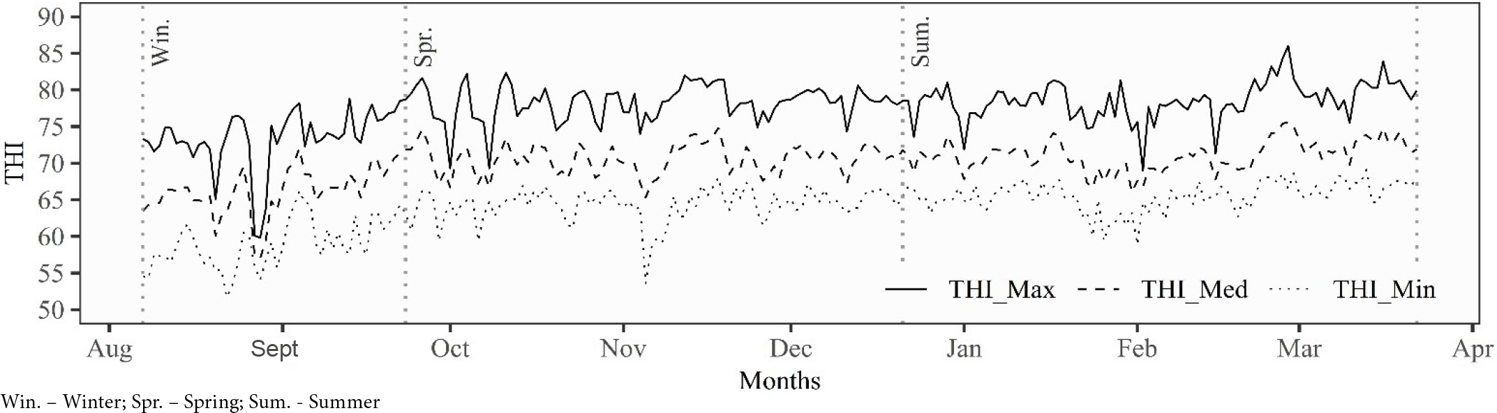
THI_Max ranged from 86.0 to 59.8, with a mean of 78.0 ± 3.5; THI_Med ranged from 75.6 to 57.0, with a mean of 70.2 ± 3.0; and THI_Min ranged from 69.1 to 51.7, with a mean of 64.7 ± 3.4 (Figure 1). A THI above 72 is considered the threshold for heat stress in Holstein cows (Becker et al., 2020; Shu et al., 2021).
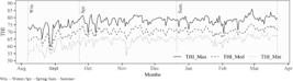
Temperature-humidity index (THI) values of the input time series, including maximum (THI_Max), mean (THI_Med), and minimum (THI_Min) values recorded during the sampling period
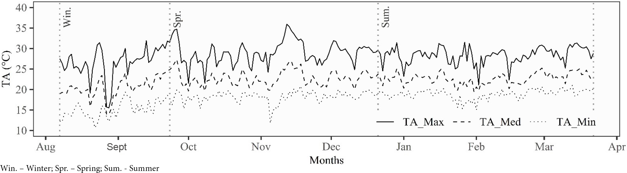
Regarding TA variation, TA_Max ranged from 35.9 to 15.5 °C, with a mean of 25.5 ± 2.8 °C; TA_Med ranged from 27.3 to 13.9 °C, with a mean of 22.3 ± 2.0 °C; and TA_Min ranged from 21.0 to 10.7 °C, with a mean of 18.4 ± 2.0 °C (Figure 2).
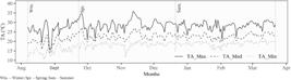
Ambient temperature (TA) values of the input time series, including maximum (TA_Max), mean (TA_Med), and minimum (TA_Min) values recorded during the sampling period
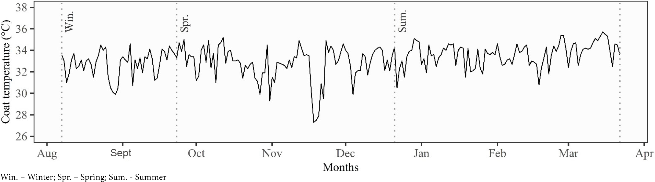
For the OTS, CT ranged from 35.7 to 27.3 °C, with a mean of 33.3 ± 1.4 °C (Figure 3).
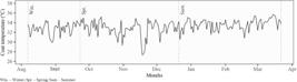
The ITS revealed a strong influence of environmental conditions on CT, with fluctuations reflecting seasonal climatic variation. CT exhibited behavior closely associated with TA, with significant increases during periods of elevated temperatures. During winter, CT remained relatively stable and substantially lower than during spring and summer, with a mean of 33.2 °C and values ranging from 32.6 to 33.8 °C.
During spring, CT showed a gradual increase, following variations in THI and, more prominently, TA, with a mean of 34.7 °C and maximum values approaching 35.6 °C. In summer, CT reached its highest levels under more severe environmental conditions, with a mean of 36.1 °C and values ranging from 35.5 to 36.9 °C. Throughout the evaluated period, CT demonstrated strong dependence on TA, with peak TA values closely aligned with maximum CT levels. Although THI also influenced CT, its association was less direct than that observed for TA. The amplitude of CT variation remained consistently lower than that of TA, which suggests a thermal buffering effect provided by the cows’ coat (Olias, 2022).
The relationship between CT and seasonal climatic variation remains insufficiently documented in the literature. Costa et al. (2023) evaluated the effects of heat stress and seasonal variation on physiological and productive responses in Holstein cows and reported that seasonal changes directly influence physiological parameters such as body temperature, CT, and milk production. Similarly, Pinheiro et al. (2005) demonstrated the physiological adaptation of dairy cows to TA variation, highlighting the correlation between TA and CT across different seasons. These findings suggest that seasonal climatic variation can be used to predict CT (OTS), supporting management strategies aimed at mitigating heat stress through the application of ARIMA models based on TF.
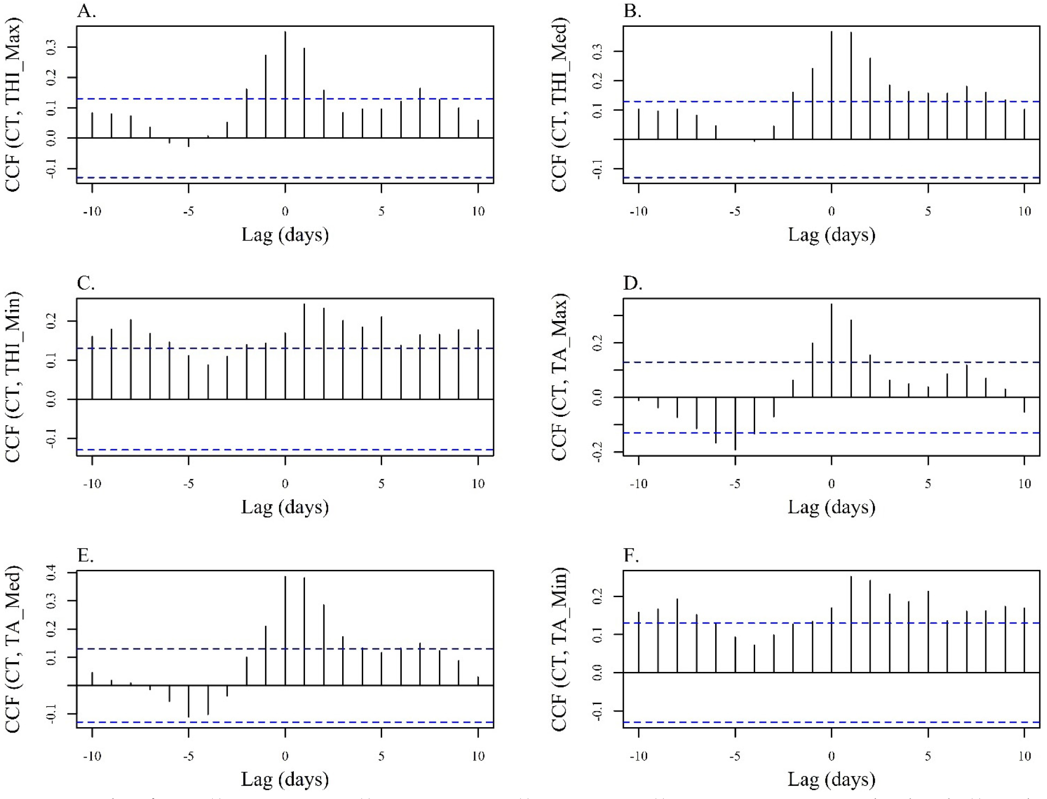
Figures 4A-F present the CCF between CT (OTS) and environmental variables (ITS). All ITS showed significant cross-correlations with CT, indicating predictive potential for estimating lagged coat temperature responses. The strength of these associations was quantified using cross-correlation coefficients, with statistically significant values exceeding confidence limits (p ≤ 0.05), as indicated by the dotted lines in the CCF plots. Lags exceeding the statistical significance thresholds were considered highly relevant (Box et al., 2015; Montgomery et al., 2015). Lagged CT responses were evident within the positive lag range (lags 1-10), with high correlation at lag 0 for all variables. The identified lag structures were as follows: THI_Max, 11 days (Figure 4A); THI_Med, 11 days (Figure 4B); THI_Min, 11 days (Figure 4C); TA_Max, 5 days (Figure 4D); TA_Med, 11 days (Figure 4E); and TA_Min, 11 days (Figure 4F).
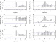
CCF between ITS and OTS: (A) CT and THI_Max; (B) CT and THI_Med; (C) CT and THI_Min; (D) CT and TA_Max; (E) CT and TA_Med; and (F) CT and TA_Min
The analysis also showed that correlations gradually weakened over time, indicating that the effects of environmental variables on CT tend to dissipate as the lag increases. In contrast, within the negative lag range, correlations were weak or absent, reinforcing that CT responds promptly to variations in THI and TA associated with heat stress. Notably, statistically significant CCF values observed at lag 0 (p ≤ 0.05) indicate an immediate and biologically relevant thermal response of CT to environmental changes. These findings emphasize the strong interaction between environmental conditions and CT.
Following the CCF analysis, stationarity tests (ADF and KPSS) were performed to determine whether the time series could be considered stationary (Table 1). Stationary series are characterized by statistical properties, such as mean, variance, and autocorrelation structure, that remain constant over time (Box et al., 2015; Montgomery et al., 2015).
Results of stationarity tests using the Augmented Dickey-Fuller (ADF) and Kwiatkowski-Phillips-Schmidt-Shin (KPSS) tests for ITS and OTS in the dynamic system
The stationarity test results indicated that only the ITS TA_Max was classified as stationary, showing statistical significance of p ≤ 0.05 in the ADF test and p ≥ 0.05 in the KPSS test (Box et al., 2015; Montgomery et al., 2015; Li et al., 2021). The ITS THI_Max, THI_Med, THI_Min, TA_Med, TA_Min, and the OTS CT were classified as non-stationary. These series were therefore transformed into stationary series using first-order differencing. However, after this transformation, the ITS lost their autocorrelation structures, effectively behaving as white noise with limited statistical information. In contrast, first-order differencing successfully transformed the OTS CT into a stationary series while preserving its autocorrelation structure.
Subsequently, the Granger causality test was performed between the selected series. The results indicated a significant causal relationship between TA_Max and CT (p ≤ 0.05) (Box et al., 2015; Montgomery et al., 2015), suggesting a rapid influence of TA_Max on CT. As lag increased, this influence progressively weakened, indicating a short-term causal relationship.
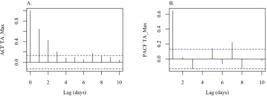
Figures 5A and B present the ACF and PACF of TA_Max, respectively. Prior to PW, it was necessary to identify the most appropriate ARIMA model for TA_Max. After evaluating different parameter combinations (p, d, q), ARIMA(3,1,3) was identified as the best-fitting model, with an AIC of 704.32. The Ljung-Box test applied to the residuals yielded p > 0.05, indicating that the residuals were independent. Furthermore, white noise analysis confirmed an adequate overall model fit (Khikmah et al., 2023). These findings support the suitability of TA_Max for predictive modeling of CT.
The PW process for the ITS TA_Max was performed according to Eq. 10. The PW(TA_Max)t series satisfied the white noise assumption based on the Ljung-Box test, with p > 0.05 (Box et al., 2015).
Where:
PW(TA_Max)t -pre-whitened ITS TA_Max (PW) %;
ϕ1, ϕ2, ϕ3 - AR coefficients (ϕ1 = - 0.47(±0.06); ϕ2 = + 0.53(±0.06); and ϕ3 = - 0.18(±0.05));
θ1, θ2, θ3 - MA coefficients (θ1 = - 0.01(±0.02); θ2 = + 0.99(±0.02); and θ3 = + 0.22(±0.02)); and,
et - random error at time t.
The PW process for the OTS CT was performed according to Eq. 11 using the same coefficients applied in the PW of TA_Max (Box et al., 2015; Montgomery et al., 2015; Li et al., 2021).
Where:
PW(CT)t - pre-whitened OTS CT (PW) %;
ϕ1, ϕ2, ϕ3 - AR coefficients (ϕ1 = - 0.47(±0.06); ϕ2 = + 0.53(±0.06); and ϕ3 = - 0.18(±0.05);
θ1, θ2, θ3 - MA coefficients (θ1 = - 0.01(±0.02); θ2 = + 0.99(±0.02); and θ3 = + 0.22(±0.02)); and,
et - random error at time t.
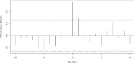
Figure 6 presents the PW-CCF between PW(TA_Max) and PW(CT). Peaks exceeding statistical significance thresholds (dotted lines) confirmed a direct and short-term causal relationship between TA_Max and CT. The highest statistically significant peak occurred at lag 0, indicating that changes in TA_Max influence CT on the same day. This finding demonstrates an immediate heat stress response in CT, which persisted for up to 48 hours until stabilization (lag 1). These results highlight the effectiveness of PW in normalizing the series and detecting causal relationships.
The recovery of CT following heat stress is gradual and influenced by several factors, including stress intensity and duration. Physiological recovery may require hours to several days depending on environmental conditions and stress severity (Nabenishi et al., 2011; Ekine-Dzivenu et al., 2020). During prolonged exposure, such as in summer, stabilization of CT tends to be further delayed (Galán et al., 2018; Herbut et al., 2018).
From a physiological perspective, CT stabilization during summer is delayed due to reduced heat dissipation efficiency, cumulative thermal load, increased metabolic activity, and insufficient nocturnal cooling (Almeida et al., 2010; Lee et al., 2015). CT generally decreases more sharply during the initial hours following heat stress and stabilizes within approximately 48 hours after stress onset (Becker et al., 2020; 2021). These findings align with Cartwright et al. (2023), who demonstrated that although other physiological parameters, such as respiratory rate, recover rapidly, CT may require 24-48 hours for full stabilization. In the present study, CT stabilized within 48 hours following heat stress cessation, consistent with prior research.
Heat stress negatively affects not only thermal recovery but also productivity, reducing dry matter intake and milk yield. These effects are most pronounced between 24 and 48 hours after stress onset (Renaudeau et al., 2012).
Based on the PW-CCF results, the TF order (r, s, b) was defined as (2, 0, 10). Parameter r = 2 indicates the number of TA_Max lags directly influencing CT; s = 0 indicates no additional CT lag structure; and b = 10 represents the maximum lag considered for TA_Max influence on CT. The selection followed the methodological framework described by Montgomery et al. (2015) and Box et al. (2015). The Eq. 12 describes the resulting TF model.
Where:
CTt and CT_pred - represent the predicted CT;
α - intercept of TA_Max (α = -0.04(± 0.20));
β - coefficient of TA_Max (β = +0.01(± 0.01));
ϕ1, ϕ2 - AR coefficients (ϕ1 = -0.47(± 0.06), ϕ2 = +0.53(± 0.06));
θ1, θ2, θ3, θ4, θ5, θ6, θ7, θ8, θ9, θ10, - MA coefficients ((θ1 = -0.01(± 0.02)), (θ2 = -0.99(± 0.02)), (θ3 = -0.28(± 0.02)), (θ4 = -0.20(± 0.02)),(θ5 = +0.05(± 0.02)), (θ6 = +0.06(± 0.02)), (θ7 = -0.01(± 0.02)),(θ8 = +0.07(± 0.02)), (θ9 = +0.03(± 0.02)), (θ10 = -0.04(± 0.02))) and,
et -random error at time t.
Figure 7 compares CT (original OTS) and CT_pred (post-TF OTS). During winter, CT ranged from 29.9 to 34.6 °C (mean 32.2 °C), while CT_pred ranged from 30.5 to 34.3 °C (mean 32.3 °C). During spring, CT ranged from 27.3 to 35.2 °C (mean 32.9 °C), while CT_pred ranged from 29.4 to 34.5 °C (mean 32.9 °C). During summer, CT ranged from 30.5 to 35.7 °C (mean 33.6 °C), while CT_pred ranged from 31.7 to 34.9 °C (mean 33.7 °C).
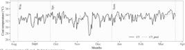
The TF model effectively captured seasonal CT trends, with CT_pred closely following observed fluctuations. Although smoothing effects were observed during periods of high thermal variability, model adherence remained strong during thermally stable periods, demonstrating robust predictive performance. The overall mean CT was 32.9 °C, while CT_pred averaged 33.0 °C, indicating strong agreement between observed and predicted values.
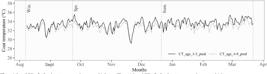
To evaluate age-related effects on CT, data were divided into two age groups: animals aged 1-3 years (CT_age_1-3 and CT_age_1-3_pred) (Figure 8) and animals aged 4-9 years (CT_age_4-9 and CT_age_4-9_pred) (Figure 9).
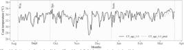
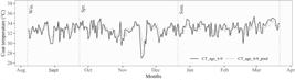
During winter, CT_age_1-3 ranged from 30.0 to 34.8 °C (mean 32.8 °C), whereas CT_age_1-3_pred ranged from 30.4 to 34.6 °C (mean 32.7 °C). In spring, CT_age_1-3 varied from 27.3 to 35.9 °C (mean 33.1 °C), while CT_age_1-3_pred ranged from 29.2 to 35.5 °C (mean 33.0 °C). In summer, CT_age_1-3 and CT_age_1-3_pred ranged from 29.8 to 36.0 °C (mean 33.7 °C) and from 31.6 to 35.4 °C (mean 33.6 °C), respectively. The overall mean for CT_age_1-3 was 33.1 °C, which was identical to CT_age_1-3_pred, indicating strong agreement between observed and predicted values.
For CT_age_4-9, winter values ranged from 29.9 to 34.4 °C (mean 32.1 °C), whereas CT_age_4-9_pred ranged from 30.5 to 34.2 °C (mean 32.3 °C). During spring, CT_age_4-9 ranged from 27.0 to 35.0 °C (mean 32.9 °C), while CT_age_4-9_pred ranged from 29.4 to 34.5 °C (mean 32.9 °C). In summer, CT_age_4-9 ranged from 29.9 to 35.4 °C (mean 33.6 °C), whereas CT_age_4-9_pred ranged from 31.5 to 35.4 °C (mean 33.9 °C). Similar to the results observed for animals aged 1-3 years, the overall means for CT_age_4-9 and CT_age_4-9_pred were identical, both at 32.9 °C.
Comparison between CT_age_1-3_pred and CT_age_4-9_pred revealed differences in the thermal responses of Holstein cows across age groups (Figure 10). Across all seasonal averages, younger animals (1-3 years) exhibited higher CT values than adult animals (4-9 years). The overall mean followed the same pattern, with CT_age_1-3_pred averaging 33.1 °C and CT_age_4-9_pred averaging 32.9 °C. These results indicate that younger Holstein cows experienced greater difficulty maintaining thermal homeostasis, particularly during summer, whereas adult Holstein cows demonstrated greater thermoregulatory efficiency, reflected by increased CT stability.
These findings suggest that the ability of Holstein cows to adapt to heat stress varies substantially with age. Younger animals typically have less developed physiological systems and less experience coping with adverse environmental conditions, including high TA and RH (Morales-Piñeyrúa et al., 2022; Zeng et al., 2023).
Additionally, younger animals exhibit more pronounced physiological responses to heat stress, including greater increases in respiratory rate, rectal temperature, and CT. These responses indicate reduced efficiency of thermoregulatory mechanisms, making younger animals more susceptible to the detrimental effects of heat stress (Frigeri et al., 2023; Zeng et al., 2023).
Adult animals, despite cumulative metabolic demands throughout their productive lifespan, tend to demonstrate greater resilience. This resilience may be associated with previous exposure to adverse environmental conditions, which promotes adaptive behavioral responses such as increased shade-seeking, preference for ventilated areas, and increased standing time to facilitate heat dissipation (Morales-Piñeyrúa et al., 2022; Frigeri et al., 2023).
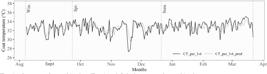
CT patterns associated with parity were also evaluated by dividing animals into two groups: cows with 1-2 calvings (CT_par_1-2 and CT_par_1-2_pred) (Figure 11) and cows with 3-6 calvings (CT_par_3-6 and CT_par_3-6_pred) (Figure 12).
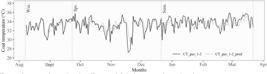
During winter, CT_par_1-2 ranged from 29.9 to 34.8 °C (mean 32.3 °C), whereas CT_par_1-2_pred ranged from 30.6 to 34.6 °C (mean 32.5 °C). During spring, CT_par_1-2 ranged from 27.2 to 35.8 °C (mean 33.1 °C), while CT_par_1-2_pred ranged from 29.5 to 35.0 °C (mean 33.2 °C). During summer, CT_par_1-2 ranged from 29.9 to 35.9 °C (mean 33.7 °C), whereas CT_par_1-2_pred ranged from 31.7 to 35.7 °C (mean 33.8 °C). Across all seasons, the overall means were similar, with CT_par_1-2 averaging 32.9 °C and CT_par_1-2_pred averaging 33.0 °C.
For cows with 3-6 calvings, winter CT_par_3-6 ranged from 29.9 to 34.4 °C (mean 32.3 °C), while CT_par_3-6_pred ranged from 30.6 to 33.9 °C (mean 32.2 °C). During spring, CT_par_3-6 ranged from 27.3 to 34.9 °C (mean 33.0 °C), whereas CT_par_3-6_pred ranged from 29.6 to 34.4 °C (mean 33.0 °C). During summer, CT_par_3-6 ranged from 29.9 to 35.1 °C (mean 33.6 °C), while CT_par_3-6_pred ranged from 31.4 to 34.4 °C (mean 33.5 °C). The overall means were statistically similar, with both CT_par_3-6 and CT_par_3-6_pred averaging 32.8 °C.
Figure 13 presents the comparison between CT_par_1-2_pred and CT_par_3-6_pred following model adjustment. During winter, CT_par_1-2_pred ranged from 30.6 to 34.6 °C, whereas CT_par_3-6_pred ranged from 30.6 to 33.9 °C. During spring, CT_par_1-2_pred ranged from 29.5 to 35.0 °C, while CT_par_3-6_pred ranged from 29.6 to 34.4 °C. During summer, CT_par_1-2_pred ranged from 31.7 to 35.7 °C, whereas CT_par_3-6_pred ranged from 31.4 to 34.4 °C.

Joint evaluation of these series indicated that cows with lower parity (LPC), including primiparous and secundiparous animals, showed greater difficulty regulating CT, with consistently higher predicted values across all seasons. This pattern indicates increased thermal sensitivity in LPC and highlights the importance of intensified thermal management strategies for this category.
Although high-parity cows (HPC) often experience cumulative metabolic demands, including increased oxidative stress related to prolonged milk production, their adaptive capacity tends to be greater than that of LPC (Frigeri et al., 2023; Zeng et al., 2023). This advantage is supported by evidence demonstrating that HPC adjust physiological and behavioral responses more efficiently, even under severe heat stress. Studies indicate that HPC exhibit lower disruption of metabolic and oxidative indicators, as well as greater stability in physiological variables such as respiratory rate and body temperature compared to LPC exposed to similar thermal environments (Morales-Piñeyrúa et al., 2022; Giannone et al., 2023; Zeng et al., 2023).
Furthermore, milk production in LPC decreases linearly with increasing THI, whereas HPC tend to maintain more stable production responses under elevated thermal conditions (Chen et al., 2022; Morales-Piñeyrúa et al., 2022; Zeng et al., 2023). These adaptive responses partially mitigate the negative effects of heat stress, contributing to improved maintenance of animal welfare and productivity (Morales-Piñeyrúa et al., 2022; Zeng et al., 2023).
Although breed effects were not directly evaluated, the observed thermal responses should be interpreted within the physiological context of Holstein cows. This European-origin breed is characterized by high milk yield and elevated metabolic heat production, which increases susceptibility to heat stress under tropical and subtropical conditions (Liu et al., 2019; Becker et al., 2020). Additionally, coat characteristics may influence heat absorption and dissipation processes in dairy cattle, thereby modulating thermal responses to environmental conditions (Morales-Piñeyrúa et al., 2022). This biological framework supports the interpretation of ageand parity-related effects observed in the present study and reinforces the need to avoid extrapolating these findings to breeds with different adaptive capacities (Li et al., 2021).
The results of this study also highlight the need for differentiated management strategies for primiparous and secundiparous cows compared with multiparous cows. Preventive interventions and enhanced cooling systems should be prioritized for younger animals, given their increased vulnerability to heat stress (Frigeri et al., 2023; Zeng et al., 2023). In contrast, cows with higher parity tend to benefit from management adjustments that reduce the impact of cumulative metabolic stress. This tailored approach may improve animal welfare and herd productivity, particularly under adverse climatic conditions, even in confinement systems (Morales-Piñeyrúa et al., 2022; Zeng et al., 2023). Therefore, understanding differences in heat stress responses among Holstein cows is essential for developing more efficient and sustainable management practices (Morales-Piñeyrúa et al., 2022; Frigeri et al., 2023; Giannone et al., 2023).
CONCLUSIONS
-
1. Seasonal climatic conditions, represented by THI and TA, directly influenced CT in Holstein dairy cows. Increases in these variables during summer resulted in higher CT values, frequently exceeding heat stress thresholds. CT exhibited a rapid thermal response to heat stress, with stabilization typically occurring within 24-48 hours, although variability was observed depending on the intensity and duration of environmental exposure.
-
2. The ARIMA (3,1,3) model combined with TF demonstrated high predictive performance for CT in Holstein cows, accurately capturing seasonal variation and lagged dynamics between environmental ITS and physiological OTS. The model also revealed differences among animal categories, with younger and lower-parity cows showing greater thermal sensitivity, whereas older and higher-parity cows demonstrated greater thermal stability, suggesting enhanced adaptive capacity.
-
3. From a practical standpoint, predictive models may support thermal management strategies by enabling anticipation of periods of increased heat stress in Holstein dairy production systems. However, application of these models should be approached cautiously, requiring validation under diverse production systems and climatic conditions, as well as cost-benefit evaluations, before large-scale implementation.
-
1
Research developed at Instituto Federal de Educação Ciência e Tecnologia do Sul de Minas Gerais - Campus Muzambinho, Muzambinho, Minas Gerais, Brazil.
-
Financing statement:
This research was funded by Coordenação de Aperfeiçoamento de Pessoal de Nível Superior (CAPES) of the Ministry of Education through the Support Program for Graduate Studies at Private Educational Institutions (PROSUP; CGCCPF 00.889.834/0001-08) as well as by the IFSULDEMINAS, process no. 23346.000157.2023-24.
-
• Ref 294454
Acknowledgments:
The authors acknowledge financial support from CAPES through PROSUP and from the IFSULDEMINAS.
Data Availability Statement:
The underlying data supporting the findings of this study are available from the corresponding author upon reasonable request (the data are part of a product currently under development).
LITERATURE CITED
-
Almeida, G. L. P. de. et al. Investimento em climatização na pré-ordenha de vacas girolando e seus efeitos na produção de leite. Revista Brasileira de Engenharia Agrícola e Ambiental, v.14, p.1337-1344, 2010. https://doi.org/10.1590/S1415-43662010001200013
» https://doi.org/10.1590/S1415-43662010001200013 -
Becker, C. A. et al. Predicting dairy cattle heat stress using machine learning techniques. Journal of Dairy Science, v.104, p.501-24, 2021. https://doi.org/10.3168/jds.2020-18653
» https://doi.org/10.3168/jds.2020-18653 -
Becker, C. A. et al. Invited review: Physiological and behavioral effects of heat stress in dairy cows. Journal of Dairy Science, v.103, p.6751-70, 2020. https://doi.org/10.3168/jds.2019-17929
» https://doi.org/10.3168/jds.2019-17929 - Box, G. E. P. et al. Time series analysis: forecasting and control. 5.ed. Hoboken, New Jersey: Wiley, 2015. 720p.
-
Cartwright, S. L. et al. Impact of heat stress on dairy cattle and selection strategies for thermotolerance: a review. Frontiers in Veterinary Science, v.10, p.1-13, 2023. https://doi.org/10.3389/fvets.2023.1198697
» https://doi.org/10.3389/fvets.2023.1198697 -
Chen, X. et al. Impact of heat stress on milk yield, antioxidative levels, and serum metabolites in primiparous and multiparous Holstein cows. Tropical Animal Health and Production, v.54. 159, 2022. https://doi.org/10.1007/s11250-022-03159-x
» https://doi.org/10.1007/s11250-022-03159-x -
Costa, D. A. da. et al. Seasonality effect on the physiological and productive responses of crossbred dairy cows to the equatorial Amazon climate. Ciência Animal Brasileira, v.24, e73559E, 2023. https://doi.org/10.1590/1809-6891v24e-73559E
» https://doi.org/10.1590/1809-6891v24e-73559E -
Dado-Senn, B. et al. Methods for assessing heat stress in preweaned dairy calves exposed to chronic heat stress or continuous cooling. Journal of Dairy Science, v.103, p.8587-8600, 2020. https://doi.org/10.3168/jds.2020-18381
» https://doi.org/10.3168/jds.2020-18381 -
Daltro, A. M. et al. Efeito do estresse térmico por calor na produção de vacas leiteiras. Pesquisa Agropecuária Gaúcha, v.26, p.288-311, 2020. https://doi.org/10.36812/pag.2020261288-311
» https://doi.org/10.36812/pag.2020261288-311 -
Ekine-Dzivenu, C. C. et al. Evaluating the impact of heat stress as measured by temperature-humidity index (THI) on test-day milk yield of small holder dairy cattle in a sub-Sahara African climate. Livestock Science, v.242, 104314, 2020. https://doi.org/10.1016/j.livsci.2020.104314
» https://doi.org/10.1016/j.livsci.2020.104314 -
Frigeri, K. D. M. et al. Effects of heat stress in dairy cows raised in the confined system: A scientometric review. Animals, v.13, 350, 2023. https://doi.org/10.3390/ani13030350
» https://doi.org/10.3390/ani13030350 -
Galán, E. et al. A systematic review of non-productivity-related animal-based indicators of heat stress resilience in dairy cattle. Plos One, v.13, e0206520, 2018. https://doi.org/10.1371/journal.pone.0206520
» https://doi.org/10.1371/journal.pone.0206520 -
Giannone, C. et al. Review of the heat stress-induced responses in dairy cattle. Animals, v.13, 3451, 2023. https://doi.org/10.3390/ani13223451
» https://doi.org/10.3390/ani13223451 -
Herbut, P. et al. Environmental parameters to assessing of heat stress in dairy cattle-a review. International Journal of Biometeorology, v.62, p.2089-2097, 2018. https://doi.org/10.1007/s00484-018-1629-9
» https://doi.org/10.1007/s00484-018-1629-9 -
Khikmah, K. N. et al. Transfer function and ARIMA model for forecasting bi rate in Indonesia. BAREKENG: Journal of Mathematics and Its Application, v.17, p.1359-1366, 2023. https://doi.org/10.1007/s00484-018-1629-9
» https://doi.org/10.1007/s00484-018-1629-9 -
Lee, Y. et al. Body temperature monitoring using subcutaneously implanted thermo-loggers from holstein steers. Asian-Australasian Journal of Animal Sciences, v.29, p.299-306, 2015. http://dx.doi.org/10.5713/ajas.15.0353
» http://dx.doi.org/10.5713/ajas.15.0353 -
Li, G. et al. Short communication: The lag response of daily milk yield to heat stress in dairy cows. Journal of Dairy Science, v.104, p.981-988, 2021. https://doi.org/10.3168/jds.2020-18183
» https://doi.org/10.3168/jds.2020-18183 -
Liu, J. et al. Effects of heat stress on body temperature, milk production, and reproduction in dairy cows: a novel idea for monitoring and evaluation of heat stress - A review. Asian-Australasian Journal of Animal Sciences, v.32, p.1332-1339, 2019. https://doi.org/10.5713/ajas.18.0743
» https://doi.org/10.5713/ajas.18.0743 - Montgomery, D. C. et al. Introduction to Time Series Analysis and Forecasting. Hoboken, New Jersey: Wiley-Interscience, 2015. 661p.
-
Morales-Piñeyrúa, J. T. et al. The effects of heat stress on milk production and the grazing behavior of dairy Holstein cows milked by an automatic milking system. Journal of Animal Science, v.100, p.1-4, 2022. https://doi.org/10.1093/jas/skac225
» https://doi.org/10.1093/jas/skac225 -
Nabenishi, H. et al. Effect of the Temperature-Humidity Index on Body Temperature and Conception Rate of Lactating Dairy Cows in Southwestern Japan. Journal of Reproduction and Development, v.57, p.450-456, 2011. https://doi.org/10.1262/jrd.10-135T
» https://doi.org/10.1262/jrd.10-135T -
Olias, C. O. Estresse térmico em vacas leiteiras: Revisão. Pubvet, v.16, p.1-4, 2022. https://doi.org/10.31533/pubvet.v16n03a1065.1-4
» https://doi.org/10.31533/pubvet.v16n03a1065.1-4 -
Pacheco, V. M. et al. Thermal imaging combined with predictive machine learning based model for the development of thermal stress level classifiers. Livestock Science, v.241, 104244, 2020. https://doi.org/10.1016/j.livsci.2020.104244
» https://doi.org/10.1016/j.livsci.2020.104244 - Pinheiro, M. da G. et al. Efeito do ambiente pré-ordenha (sala de espera) sobre a temperatura da pele, a temperatura retal e a produção de leite de bovinos da raça Jersey. Revista Portuguesa de Zootecnia, v.12, p.37-43, 2005.
-
Renaudeau, D. et al. Adaptation to hot climate and strategies to alleviate heat stress in livestock production. Animal, v.6, p.707-728, 2011. https://doi.org/10.1017/S1751731111002448
» https://doi.org/10.1017/S1751731111002448 -
Shu, H. et al. Recent advances on early detection of heat strain in dairy cows using animal-based indicators: A review. Animals, v.11, 980, 2021. https://doi.org/10.3390/ani11040980
» https://doi.org/10.3390/ani11040980 -
Zeng, J. et al. Heat stress affects dairy cow health status through blood oxygen availability. Journal of Animal Science and Biotechnology, v.14, 112, 2023. https://doi.org/10.1186/s40104-023-00915-3
» https://doi.org/10.1186/s40104-023-00915-3
Edited by
-
Editors:
Edivan Rodrigues de Souza & Carlos Alberto Vieira de Azevedo

 Win. - Winter; Spr. - Spring; Sum. - Summer
 Win. - Winter; Spr. - Spring; Sum. - Summer
 Win. - Winter; Spr. - Spring; Sum. - Summer
 CCF - Cross-correlation function; ITS - Input time series; OTS - Output time series; CT - Coat temperature; THI_Max - Maximum temperature-humidity index; THI_Med - Average temperature-humidity index; THI_Min - Minimum temperature-humidity index; TA_Max - Maximum ambient temperature; TA_Med - Average ambient temperature; TA_Min - Minimum ambient temperature
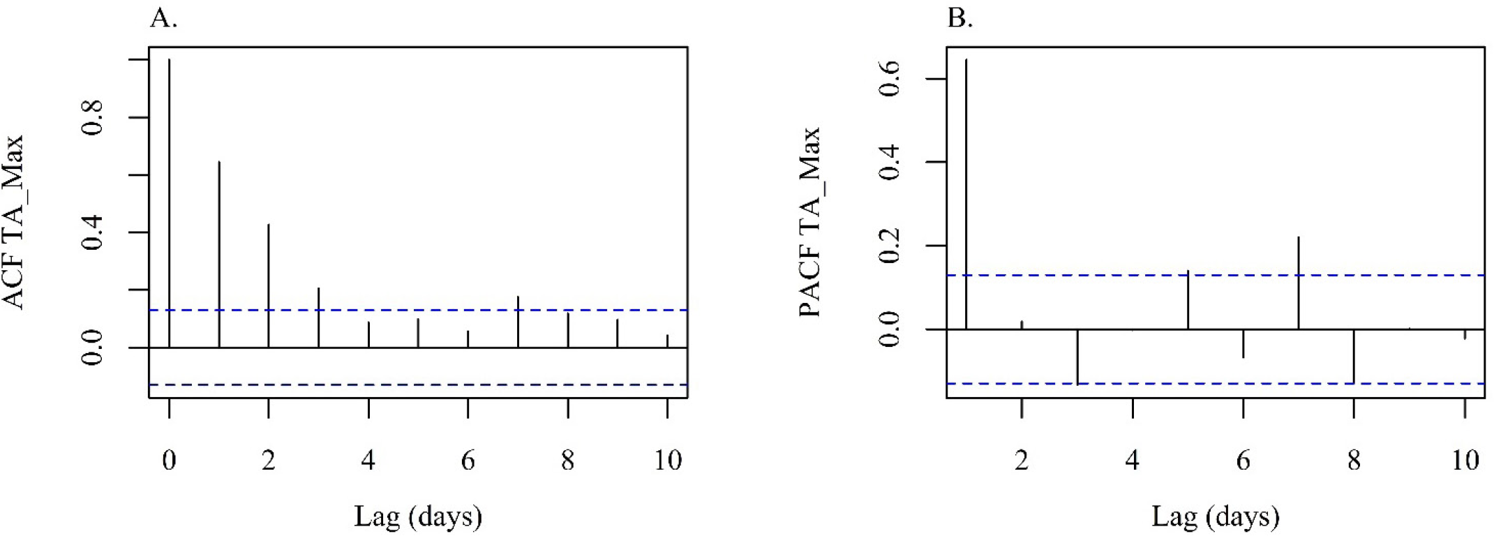 ACF - Autocorrelation function; TA_Max - Maximum ambient temperature; PACF - Partial autocorrelation function; For interpretation, peaks that exceed the dotted lines are considered significant autocorrelations
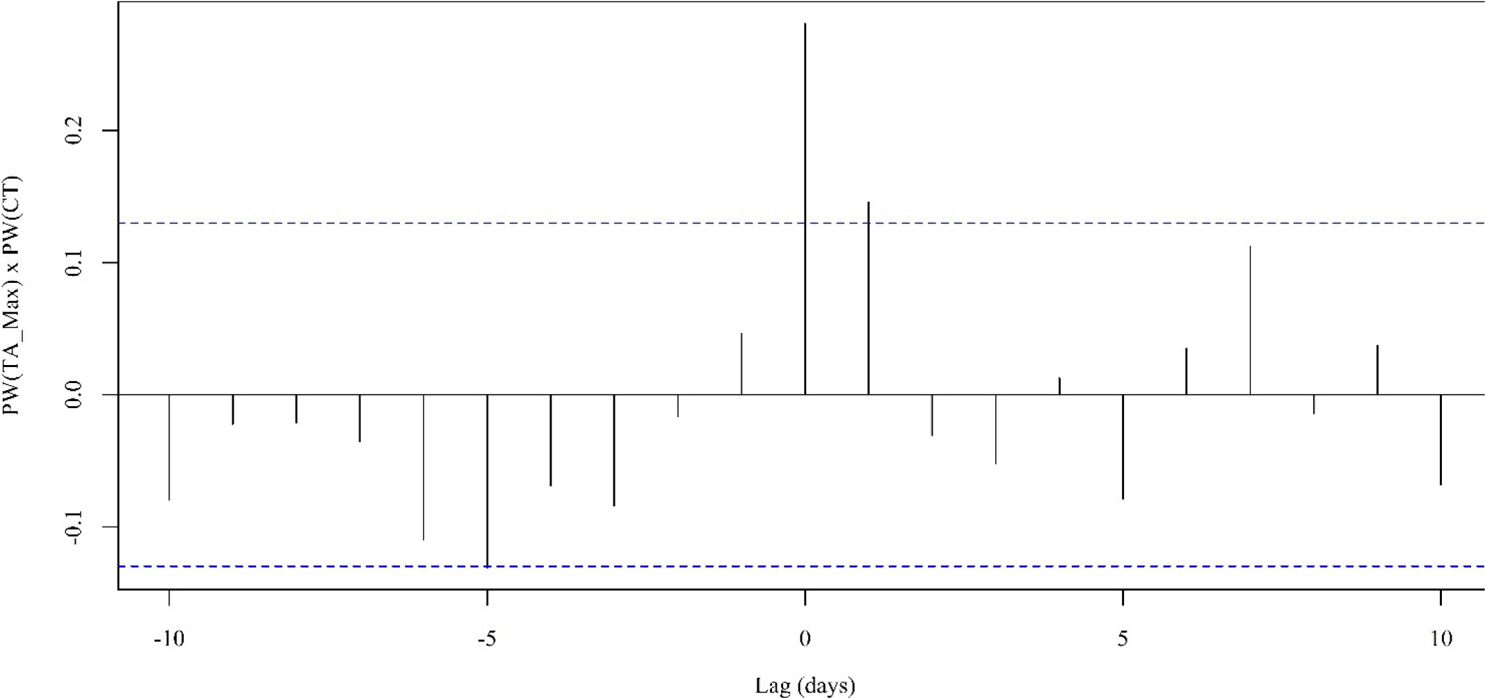 PW-CCF - Pre-whitened cross-correlation function; ITS PW(TA_Max) - Input time series pre-whitened of maximum ambient temperature; OTS PW(CT) - Output time series pre-whitened of coat temperature
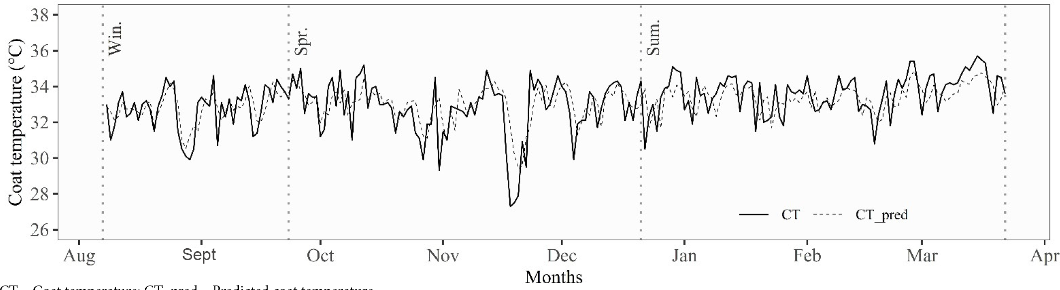 CT - Coat temperature; CT_pred - Predicted coat temperature
 CT_age_1-3 - Coat temperature for animals aged 1-3 years; CT_age_1-3_pred - Predicted coat temperature for animals aged 1-3 years
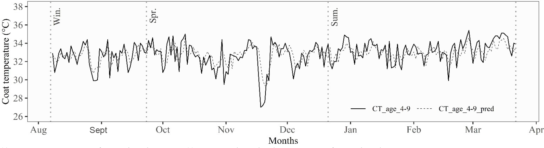 CT_age_4-9 - Coat temperature for animals aged 4-9 years; CT_age_4-9_pred - Predicted coat temperature for animals aged 4-9 years
 CT_age_1-3_pred (°C) - Predicted coat temperature for cows aged 1-3 years; CT_age_4-9_pred (°C) - Predicted coat temperature for cows aged 4-9 years
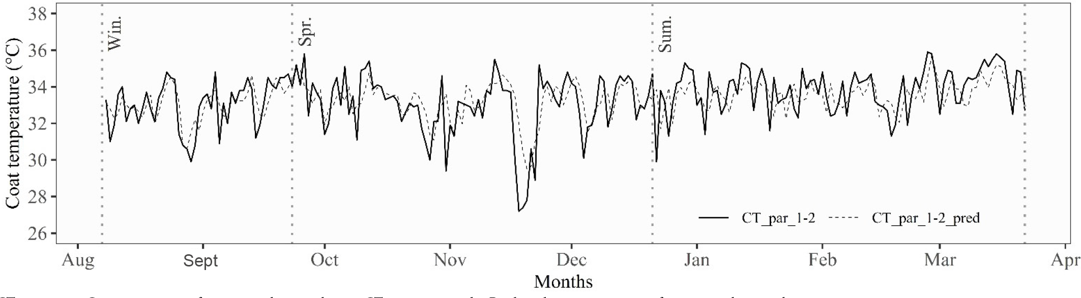 CT_par_1-2 - Coat temperature for cows with 1-2 calvings; CT_par_1-2_pred - Predicted coat temperature for cows with 1-2 calvings
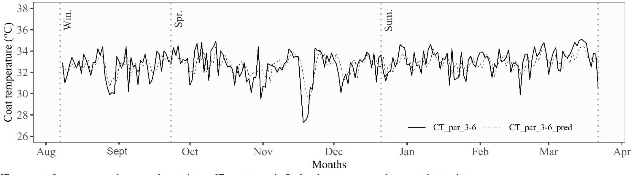 CT_par_3-6 - Coat temperature for cows with 3-6 calvings; CT_par_3-6_pred - Predicted coat temperature for cows with 3-6 calvings
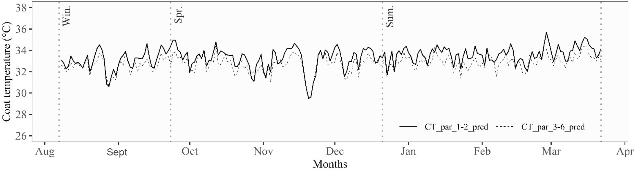 CT_par_1-2_pred - Predicted coat temperature for cows with 1-2 calvings; CT_par_3-6_pred - Predicted coat temperature for cows with 3-6 calvings