Prediction of healthcare costs on consumer direct health plan in the Brazilian context

Resumo

The rise in healthcare costs has led to the adoption of cost-sharing devices in health plans. This article explores this discussion by simulating Health Savings Accounts (HSAs) to cover medical and hospital expenses, supported by catastrophic insurance. Simulating 10 million lives, we evaluate the utilization of catastrophic insurance and the balances of HSAs at the end of working life. To estimate annual expenditures, a Markov Chain approach - distinct from the usual ones - was used based on recent past expenditures, age range, and gender. The results suggest that HSAs do not create inequalities, offering a viable method to sustain private healthcare financing for the elderly.

JEL classification. I13, C02, C15, C53.

1. Introduction

Consumer directed health plans (CDHP) are products intended to fund healthcare expenses, which have been consolidated in the United States since the end of the nineties as a possible approach to contain the rise in healthcare costs. In CDHP, the insured has a personal account to pay for his or her medical procedures, what leads to the increase in awareness about healthcare costs (Gabel et al. (2002) and Bundorf (2016)).

According to Bundorf (2016), there are three features often associated to CDHP: relatively high deductibles, a personal account to accumulate resources, and availability of information about healthcare costs. On the one hand, these features diverge from models based purely on mutualism, as they seek to accomplish a higher perception of well-being and economy efficiency, while mitigating the disruptive impacts due to moral hazard. On the other hand, the attachment of individual expenses to a personal account raises questions about justice, as individuals could persistently experience health shocks during their work life, making it unlikely for them to save enough to cover their expenses after retirement. This would cause, from a population point of view, a great variation on the balance of these accounts, causing a part of the population to have a great amount of resources at retirement (savings), while other part would not have accumulated anything (the product would have features of a self-insurance) (Eichner, 1998).

In recent years, a great rise in healthcare costs has been observed around the world. In the Brazilian supplementary health system, for example, the mean annual healthcare expense, including dental benefits, increased 73% between 2013 and 2018 according to the National Supplementary Health Agency (ANS, 2019-2021a), what has led to a public debate about the sustainability of the sector (ANS, 2019-2021b). Following the example of other countries, it has been proposed an alternative to the system in an attempt to establish norms and legal certainty for products with co-payment and deductible devices, as it is a reasonable assumption that Brazil faces similar challenges as other countries in what concerns the essential cause of healthcare costs increase, that is, spending more than needed to treat a specific health problem. This over-consumption and oversupply pattern is understood as the result of two factors. On the one hand, consumers may partake in more risky activities when protected by a health plan, increasing the probability of needing more care (ex-ante moral hazard) or simply consuming more care than necessary (ex-post moral hazard). On the other hand, providers may supply more care than needed, inducing the demand (Ehrlich and Becker (1972) and Zweifel and Manning (2000)).

In order to mitigate the impact of these factors, in 2018 the Brazilian regulatory agency (ANS) proposed a resolution to regulate co-payment and deductibles in health plans (RN nº 433, June 27 2018), which had a negative public repercussion, that led ANS to suspend the norms, leaving the market uncovered in what concerns the understanding of these devices. The negative repercussion was caused by a misunderstanding about the real use of these devices in health plans, what evidences the need to further the discussion about them, including the possibility of considering them as part of a new market segment.

This paper aims to subsidize the discussion with the analysis of empirical data by simulating health savings accounts (HSA). A product derived from CDHP, the HSA are individual accounts set to exclusively cover expenses with healthcare goods and services, which is composed by a resources accumulation phase, typically subsidized by the employer with participation of the employee, followed by a decumulation phase, generally after retirement. The objective of this form of funding is the implementation of a risk pooling over the individual cycle of life, mobilizing resources from various sources to fund the decumulation phase. Resource mobilization to a savings account for the stages of the life cycle when the increase in healthcare expenses exceeds income is a response to policies aimed at maintaining private funding for healthcare for the elderly population.

Since the end of the nineties, countries as the United States, China, Singapore and South Africa have taken steps to incorporate these alternatives in their health systems. In the US experience, the HSA products combine a high deductible health plan with tax breaks to form a savings account. These products have a mixed framework, which seeks to reduce the individual exposition to the risk of extreme events, by combining two devices: a catastrophic health insurance associated with a personal savings account.

In this paper, we simulate a HSA product combined with a catastrophic health insurance during a labor period of forty years (from 25 to 65 years-old) in the Brazilian context. The main objective of the simulation is to study, from a population point of view, the variation of HSA balances at the end of the accumulation phase. A great discrepancy in these balances may be interpreted as the result of persistent health shocks, understood here as the cause of the financial need for healthcare goods and services, and measured through the costs covered by a health plan under the individual perspective. The persistence of shocks is a fundamental aspect in the debate about CDHP since one could argue that individuals with poor health would not be able to accumulate savings overtime, so these accounts would reflect inequalities between individuals with distinct overall health conditions.

In order to simulate the annual healthcare expenses of an individual, we propose an approach based on Markov Chains (Taylor and Karlin, 1998), which differs from the usual methods of predicting healthcare expenses based on regression models (Jones, 2000). In this approach, we define levels of annual expense, which are ranges of expense, and apply a prediction technique which estimates the probability of an individual to have annual expenses in each level, based on his or her levels in the previous two years, age range and sex. This model does not try to predict the exact value of the annual expenses by assuming some kind of functional relation between the expenses and the independent variables, but rather predicts the probability of each level of expense for each combination of categories of the independent variables sex, age range and previous expense levels.

Freed from assumptions about regression error distributions and the restricted form of the functional relation between dependent and independent variables, which are often not satisfied in real datasets, a Markov Chain approach makes a mild assumption about the dependence between the expenses in a year with that in previous years, and tries to achieve a more realistic goal, which is to predict an expense level rather than the exact value of the expense. This more realistic approach may lead to improved prediction models, as it can be applied in the context of any country and naturally considers their specific behaviors.

In Section 2 we present the dataset used in the simulation, and discuss the considered CDHP product, the modelling of healthcare expenses and the proposed Markov Chain approach. In Section 3 we present the results of the simulation studies, and in Section 4 we comment on how they may be interpreted to subsidize the debate about CDHP products in Brazil.

2. Materials and methods

2.1 Dataset

The dataset contains claims of a Brazilian self-management health plan. There are six types of health plans operators in Brazil, which are characterized by the juridical nature of their operations. The self-management health plans are similar to the self-insured group health plans in the US, which offer plans for employees and dependents, assuming the financial risk, which can be partially funded by the employees. This portfolio was followed longitudinally for five years (2005 to 2009) and all claims (expenses) are corrected by the inflation index IPCA (Extended National Consumer Price Index) to the December 2009 value.

As the objective of this paper is to study the persistence of health shocks during the work life, we will consider only working age individuals, that is, those with 25 years completed at January 2005 and with at most 65 years completed at December 2009, which amounts to approximately 39,000 lives. During the five years of study, the portfolio size changed because of the entrance of new individuals, death and other motives, so from all these lives, around 11,000 were not followed during all the period, so there will be considered in the analysis only the 27,780 individuals between 25 and 65 years-old which were in the portfolio for the whole period.

Table 1 presents some descriptive statistics of the annual expenses of the individuals within the considered age range which stayed in the portfolio during the five-year period. The percentage of individuals with zero annual expenses is between 5 and 6% in all years. As Table 1 portrays the behavior over time of a closed cohort, it is expected that a shift in the mean expense occurs due to the aging of the group. However, even though the variation in the mean expense from 2005 to 2009 was around 36% and the expenses are corrected by a general inflation index, there is no guarantee that the real variation due to aging can still be observed in the costs of the healthcare goods and services of this portfolio. Therefore, in reality, both the aging effect and the real variation in the costs are reflected in these values.

Table 1
Descriptive statistics of the annual expenses of individuals between 25 and 65 years-old which stayed on the portfolio during the whole five-year period. The percentiles, mean and standard deviation are calculated considering only the individuals with positive expenses.

Description	2005	2006	2007	2008	2009
n	27,780	27,780	27,780	27,780	27,780
PctNoExpense	5.97	5.52	5.77	5.55	5.76
p25	319	303	332	368	359
p50	764	736	791	904	872
p75	1,746	1,666	1,789	2,090	2,008
p90	3,993	3,735	4,130	4,861	4,761
p95	7,083	6,531	7,477	8,726	9,114
p96	8,497	7,960	8,864	10,247	10,780
p97	10,450	9,853	10,935	12,910	14,190
p98	13,538	13,134	15,380	18,237	20,160
p99	22,910	21,683	25,851	31,158	33,730
p995	33,905	35,695	43,747	54,407	55,601
p999	92,962	105,585	92,549	139,811	181,947
max	426,772	528,293	355,220	1,044,525	965,287
mean	2,064	2,041	2,220	2,710	2,813
sd	6,833	8,127	7,536	11,612	12,673

• n: total of individuals in portfolio; p(k): k-th sample percentile; sd: standard deviation.

As expected (Seshamani and Gray (2004), Zweifel et al. (2004) and Werblow et al. (2007)), large expenses are concentrated in a small parcel of individuals: in 2008, lesser than 1% of the individuals were responsible for expenses ranging from R$ 31,158 to R$ 1,044,525 where we observe that the maximum expense is 385 times the mean one. Also, in 2005, around 5% of the individuals were responsible for annual expenses ranging from R$ 7,083 to R$ 426,772, and the maximum expense was 206 times the mean one.

In orderto compare men and women according to their annual expenses, we present in Tables A.1 and A.2 in Appendix A some descriptive statistics for the annual expenses for each sex. From the total of individuals, there are 13,539 (49%) women and 14,241 (51%) men. Over time, the percentage of women without expenses ranged between 5.1 and 5.5%, while the percentage of men ranged from 5.8 to 6.8%. When considering only the individuals with positive expense, we see that the mean annual expenses of women is greater than that of men, as it varied between R$ 2,341 and R$ 3,062 for the female sex, and between R$ 1,795 and R$ 2,576 for the male sex. In the same manner, the median annual expenses of women ranged from R$ 998 to R$ 1,104 and that of men from R$ 580 to R$ 721.

In Tables A.3, A.4, A.5, A.6, A.7, A.8, A.9, A.10, A.11, A.12, A.13, A.14, A.15, A.16, A.17, A.18, A.19, A.20 in Appendix A we present the descriptive statistics of the annual expenses by sex and age range, where it can be seen in all years that the mean annual expenses increase with age, highlighting the effect of age range on healthcare expenses. When we assess the factors which influence individual healthcare expenses, age is always presumed to have a positive effect since, as age increases, so does the probability of occurrence of chronicle diseases and loss of functional capabilities. Therefore, it is expected that high expenses are related to advanced age (Duncan et al. (2016) and Frees et al. (2014)).

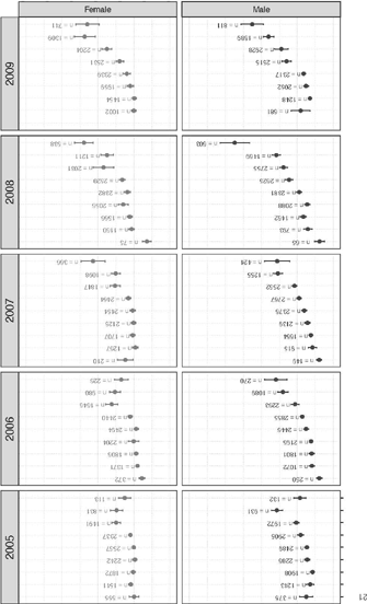
In Figure A.1 in Appendix A we present the mean annual expenses for each combination of sex and age range, with an error bar representing one standard error. On top of each error bar, we present the size of each group. When we compare men and women, we see a distinct pattern, as women tend to spend more in the early age ranges, a tendency which inverts itself in later ranges. This feature is found in other references in the literature (Yamamoto, 2013). Over time, we observe a greater increment in the expenses of the later age ranges.

While the mean annual expenses of men increase constantly with age, the mean annual expenses of women is stable until the age of 50, when we see an increase in the mean of the age ranges 51-55 and 56-60, followed by a small reduction in age range 61-65. Thus, we see that women spend more than men in practically all age ranges, although this difference decreases with age. In 2006 and 2008, the mean annual expenses of men in the age range 61-65 surpassed that of women.

2.2 Persistence of costs

Persistence of costs is defined as the continuity (permanence) of elevated health costs of an individual over time. In order to analyze the persistence of costs, we divide the individual annual expenses of each year i ∈ {2005,2006,2007,2008,2009} into four levels, namely:

• F_1,i: annual expenses lesser or equal to R$ 300 at year i;

• F_2,i: annual expenses greater than R$ 300 and lesser or equal to R$ 1,000 at year i;

• F_3,i: annual expenses greater than R$ 1,000 and lesser or equal to R$ 5,000 at year i; and

• F_4,i: annual expenses greater than R$ 5,000 at year i.

Dividing the expenses this way we have, for each individual, a sequence of five levels describing his or her expenses throughout the years. For example, an individual with costs {0;200;500; 1,500;200} has sequence F_1,2005, F_1,2006, F_2,2007, F_3,2008, F_1,2009 as expense levels.

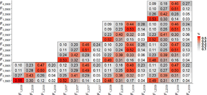
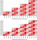
In Figure 1 we present the sample proportion of individuals which transitioned between each pair (F_k,i, F_l,j), j > 1 of states, in which rows represent the origin state F_k,i and columns the destination state F_l,j. The color of the matrices entries is related to the estimated transition probability: red means great probability (around 0.5), gray means medium probability (around 0.2) and white means low probability (around zero). In this figure, there are ten 4 by 4 matrices, one for each pair of distinct years, which present the transition probabilities from the ranges of the early year to that of the later. For example, the matrix in the lower-left corner presents the transition probabilities between the expense’s levels of 2005 and 2006, and the matrix in the upper between the expense’s levels of 2008 and 2009. The leading diagonal of each matrix is the proportion of individuals which stayed at the same expense level at both years.

Figure 1
Transition matrix of expenses for each two years combination.

In Figure 1 we see, for example, that within individuals with expenses greater than R$ 5,000 in 2008, 46% had expenses between R$ 1,000 and R$ 5,000, and 27% maintained the expenses at level greater than R$ 5,000, in 2009; within individuals with annual expenses lesser or equal to R$ 300 in 2007, 52% had expenses lesser than R$ 300, and only 3% had expenses greater than R$ 5,000, in 2008. We also note that high values of probabilities are concentrated around the leading diagonals, except at the greatest expense level. However, these high values decrease with the distance between the years, highlighting the fact, also observed in Eichner et al. (1996), that persistence of costs decays over time. It is important to note that the matrices were constructed considering only the individuals between 25 and 65 years-old that were alive in 2009. If the individuals which died in the considered period were also considered, then there would be greater probabilities in the diagonal point of the greatest expense level, as it is known that individuals tend to have consistently high expenses in the period leading up to their death.

In order to evaluate the effect of age on the persistence of costs, we present in Fig. A.2 in Appendix A the transition matrices calculated considering only the younger (21 to 40 years-old) and older (41 to 65 years-old) individuals, respectively. When comparing the diagonal of the matrices of both figures, we see that, for younger individuals, the probability of those in expense level 3 remaining in the same level or moving up to expense level 4 is approximately 56%. However, for the population aged 40 and above, this proportion is around 66%, i.e., 10 percentage points higher, in average.

2.3 Health Savings Accounts (HSA)

The health savings accounts (HSA) are devices in which a savings account attached to each individual receives annual contributions with the exclusive purpose of covering healthcare expenses. The annual expenses covered by HSA are limited by a predefined value while its balance is positive. In case expenses exceed the limit or the account balance, then a catastrophic insurance is activated to cover them. Although there is a limitation on the expenses covered by funds from the savings account, in this device there is no limitation on individual annual healthcare expenses, as the insurance covers any expenses beyond the threshold.

The CDHP product considered in this paper is a HSA in which each individual has an account, started at 25 years-old, from which are deducted his or her healthcare expenses. The account dynamic is as follows:

• At the beginning of each year, the employer deposits R$ 2,500 on the individual account.

• In case the annual healthcare expenses of an individual do not exceed the account balance or R$ 5,000, they are fully paid by funds from the account. If the annual expenses surpass R$ 5,000 or the balance of the account, then R$ 5,000, or the balance, is withdrawn to partially cover them, and the remaining value is covered by a catastrophic insurance. Therefore, all healthcare expenses up to R$ 5,000 or the account balance, if lesser, are covered by the individual, and the remaining value is covered by the insurance.

In what follows, we present an approach based on Markov Chain to simulate the product described above, which seeks to predict the expense level of each individual at each year of his or her work life in order to assess the balance of the accounts at age 65, and the frequency and severity of catastrophic insurance use, from a population point of view. In the next section, we discuss the approaches to healthcare expenses prediction at the individual level used in the literature, presenting their qualities and shortcomings.

2.4 Prediction of future healthcare expenses at individual level

Modelling techniques to assess the risk associated with events which incur in healthcare expenses are relatively recent (Jones, 2000), for their development is dependent on the volume and quality of available information, which have only improved in the last couple of decades. Also, the sector has been demanding new frameworks for covering and management of health risks, in contrast to its historical foundation, based purely on refunding, increasing the need for improved quantitative models.

In order to model healthcare expenses patterns in the US, Frees et al. (2011) considered more than thirty factors related to an individual’s demography, socioeconomic level, health condition, employment and availability of health insurance. There were considered two dependent variables, namely, frequency and severity of expenses, and the significant factors found for each of them differed. Also, Duncan et al. (2016) explored the effects on healthcare expenses of approximately one hundred independent variables related to demography, age and comorbidities history, among others.

Pope et al. (2004) and Duncan et al. (2016) pointed out the limitations of models which consider only demographic factors and health condition history, affirming the importance of taking into account past expenses while developing prediction models. Indeed, according to Duncan et al. (2016), one of the best sources of information for predicting healthcare expenses are past expenses.

About issues encountered when modelling individual healthcare expenses, Duncan et al. (2016) evidenced that: (a) annual expenses follow approximately a log-normal distribution and are characterized by high variance; (b) the error distribution is clearly heteroscedastic: the conditional variance for individuals with high expenses is greater than that of individuals with low expenses; (c) there exists interaction between the independent variables, and the relationship between expenses and health condition is expected to be non-linear, what implies non-linear relationships between dependent and independent variables; (d) many of the independent variables are highly correlated and some of them have very rare categories. Due to the great variability of annual expenses in a population and the great number of independent variables, the quality of fitted models is quite low.

Other problems encountered when modelling annual healthcare expenses are the excess of zeros and the presence of extreme values. The first problem is due to individuals which do not use their health insurance in the period of a year. The second is caused by the fact that a very small portion of a population has annual expenses hundreds of times the mean one. In order to attack these problems, Marcondes et al. (2018) proposed a hurdle model for heavy-tailed data, which is specifically useful for annual healthcare expenses data. A hurdle model takes special care of the zero values, while a heavy-tail model takes into account values far from the mean. The mixture of models treating these two features is a better fit for annual healthcare expenses than the usual regression models, as evidenced by the application in Marcondes et al. (2018), which considered a dataset of annual healthcare expenses.

Based on the literature, we see that there is a need to develop better techniques to model healthcare expenses in a dynamic scenario characterized by the rapid increase in the amount of available information and data about individuals. With this purpose, we consider a Markov Chain approach to model healthcare expenses in order to simulate an HSA product.

2.5 Methodology for prediction of future healthcare expenses at individual level

In this section, we present the methodology proposed in this paper to predict future healthcare expenses at the individual level, which is based on Markov Chains of order 2 that are defined in Appendix B. The prediction technique will be employed to estimate annual individual healthcare expenses in order to simulate the expenses which will be covered by a HSA during the labor life of simulated individuals.

2.5.1 Simulation of individual annual healthcare expenses over time

Our simulation study is based on the assumption that the pattern of annual healthcare expenses of an individual is similar to that of those of the same sex, age range and expenses history. The study consists in the simulation of 10,000 lives, starting at 25 years-old, which are followed annually until 65 years-old, what corresponds to the forty-one years of a work life. The annual expenses of these individuals in their first year (25 years-old) are sampled from the 2009 annual expenses empirical distribution of age range 25-30. There are 1,683 individuals in the age range 25-30 in 2009, so in order to obtain 10,000 lives from them, we will sample 10,000 lives with repetition from the 1,683 individuals, setting the age of all new sampled individuals to exactly 25 years-old.

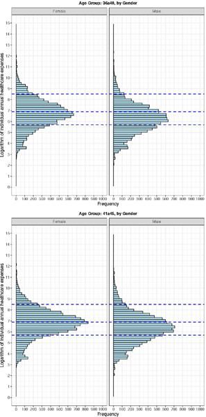
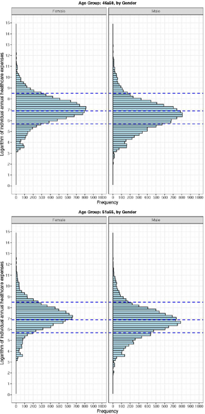
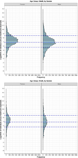
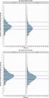
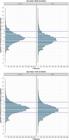
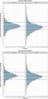
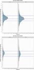
From the sex, age range, expenses history and expenses in the first year of the 10,000 lives, we simulate their personal HSA over time, a process fulfilled by iterating two consecutive procedures. In the first step, we predict to which expense level each individual will go, based on probabilities depending on his or her sex, age range at the present year and expense level on the current and previous year. On the second step, we sample the exact value to be deducted from each individual account to cover the expenses from the empirical distribution of the annual expenses of the individuals of the same sex, age range and predicted expense level. This empirical distribution is the one in Fig. B.1 which is related to the individual’s age range and sex. The distribution is built by combining individual’s medical expenses from years 2005 to 2009, stratified by age and sex, obtaining the possible points that can be sampled within the expense level sampled in the first step, i.e., between the respective dotted lines in Fig. B.1. The simulation was replicated i,000 times. In Appendix B, we further explain the simulation dynamics.

3. Results

In order to assess the effectiveness of the HSA, we present in this section the results of the simulation study regarding the balance of the individual accounts over time, and the frequency and severity of the catastrophic insurance use.

3.1 Balance of the individual health savings accounts

In Table 2 we present descriptive statistics of the individual HSA of the simulated 10,000 lives at every five years between 25 and 65 years-old.

Table 2
Descriptive statistics of the simulated individual mean HSA balance at every five years between 25 and 65 years-old. We present the mean (µ) and standard deviation (σ) over the 1,000 simulations.

	25-30		31-35		36-40		41-45		46-50		51-55		56-60		61-65
	µ	σ	µ	σ	µ	σ	µ	σ	µ	σ	µ	σ	µ	σ	µ	σ
no	2,693	46.38	496	21.93	227	14.92	144	11.69	121	10.89	123	10.53	126	10.61	133	11.61
P5	1,058	14.09	2,907	71.85	5,138	125.04	7,434	174.39	9,238	214.90	10,232	248.86	10,734	278.85	10,706	294.34
p10	1,593	16.48	4,711	72.43	7,961	122.21	11,123	166.51	13,734	202.02	15,413	237.51	16,479	263.42	16,807	280.47
p15	1,960	12.16	6,165	77.60	10,056	118.58	13,810	161.58	16,966	190.51	19,139	221.65	20,622	251.52	21,249	271.23
p25	2,385	6.84	8,467	75.27	13,298	111.78	17,930	141.20	21,876	173.91	24,800	204.01	26,927	233.74	28,062	254.14
p40	3,993	22.48	11,214	70.06	17,117	101.10	22,734	127.61	27,598	157.55	31,423	188.78	34,341	217.03	36,126	238.85
p50	4,723	14.96	12,846	65.88	19,359	95.41	25,535	123.00	30,934	150.65	35,309	179.50	38,721	206.08	40,932	231.85
p75	7,843	39.48	16,608	53.84	24,777	82.13	32,278	109.82	39,016	135.52	44,831	167.13	49,603	193.85	53,051	227.11
p85	9,404	23.11	18,587	50.79	27,201	73.21	35,361	102.83	42,753	133.39	49,286	164.03	54,800	189.26	58,949	230.20
p95	11,792	22.48	21,663	56.93	30,869	76.88	39,728	101.04	48,068	132.23	55,699	168.59	62,406	209.51	67,718	253.78
p98	13,193	29.56	23,301	46.22	32,987	77.81	42,280	103.93	51,064	140.66	59,313	181.59	66,747	238.78	72,770	291.57
max	14,621	50.65	26,407	114.55	37,976	194.88	49,347	318.00	60,427	526.57	71,231	762.78	81,510	1,064.25	89,269	1,342.32
mean	5,446	20.08	12,571	50.98	18,858	74.16	24,831	95.64	30,115	115.29	34,478	134.69	37,971	151.71	40,345	168.52
sd	3,410	8.89	5,613	24.45	7,780	39.52	9,799	53.11	11,769	65.71	13,756	79.44	15,599	91.95	17,186	102.92

• n₀: total of individuals with zero balance in HSA; p(k): k-th sample percentile; SD: standard deviation.

According to the simulation, at 30 years-old 26% of the lives had a zero balance in their HSA and, at 40 years-old, this percentage was lesser than 3%, in average. As the annual health expenses are smaller at young age, the mean increase in the individual HSA balance is greater in early ages, and in later age ranges this balance is more spread around the mean. At 40 years-old, only 5% of the lives had a balance greater than R$ 30,000 in average and, at 45 years-old, between 50% and 75% of the lives had this kind of balance. At 55 years-old only 15% of the lives had a balance lesser than R$ 20,000, while 15% had a balance greater than R$ 50,000 in average and, at 60 years-old, only 25% of the lives had a balance lesser than R$ 30,000 in average and 50% had a balance greater than R$39,000 in average.

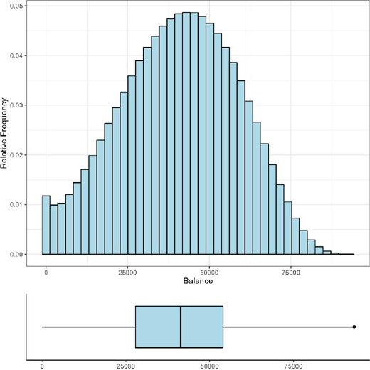
At 65 years-old, the end of the work life, only 1% of the lives had zero balance and 5% a balance lesser than R$11,000 in average, while half the lives had a balance greater than R$41,000 in average, with 25% with a balance greater than R$53,000 in average. The mean balance at 65 years-old is around R$40,000 in average, with a maximum balance around R$89,000 in average. In Fig. 2 we present the empirical distribution of the individual HSA balance in the 10,000,000 simulated individuals at 65 years-old. This distribution is approximately symmetrical (Skewness coefficient = -0.1202) and 01 outlier was detected (R$93,142.83). According to the simulation, the HSA is a good alternative to fund healthcare costs at old age, as a great parcel of the simulated population had a considerable balance at retirement. Note that the simulation is based on the expenses of a portfolio in which there is no individual HSA, and that we considered a savings account without interest. Therefore, the balance of the individual HSA could in reality be greater than that simulated.

Figure 2
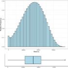
Empirical distribution of the simulated HSA balances at 65 years-old of the 10,000,000 simulated individuals.

3.2 Frequency and severity of the catastrophic insurance use

In this section we analyze the use of the catastrophic insurance, more specifically its frequency and severity. In Table 3 we present the percentage (frequency), and the total value covered (severity), of the lives which used the catastrophic insurance each number of times.

Table 3.
Mean Frequency and severity of the catastrophic insurance use by the simulated lives during the 40 years period. We present the mean (µ) and standard deviation (σ) over the 1,000 simulations.

No. of Times	n		(%) of Usage		Tot. CI Usage		Mean Usage per live
	µ	σ	µ	σ	µ	σ	(%) CI Usage	Cum.(%) of Usage	Cum.(%) CI Usage	µ	σ
0	559	23.19	5.59	0.23	0	0	0.00	5.58	0.00	0	0
1	1,152	31.78	11.52	0.32	14,706,212	1,106,298	3.01	17.10	2.99	12,760	882
2	1,474	36.82	14.74	0.37	36,720,303	1,876,230	7.50	31.82	10.46	24,919	1,079
3	1,510	36.43	15.10	0.36	55,345,252	2,439,868	11.31	46.91	21.72	36,648	1,323
4	1,361	33.12	13.61	0.33	65,156,889	2,701,662	13.32	60.50	34.97	47,885	1,603
5	1,121	32.67	11.21	0.33	65,797,506	2,987,801	13.45	71.71	48.35	58,667	1,975
6	867	28.40	8.67	0.28	60,042,438	2,939,841	12.27	80.36	60.56	69,293	2,533
7	636	24.31	6.36	0.24	50,631,601	2,721,570	10.35	86.72	70.86	79,608	3,089
8	446	20.18	4.46	0.20	39,977,371	2,576,693	8.17	91.17	78.99	89,615	4,112
9	302	16.89	3.02	0.17	29,969,236	2,245,427	6.12	94.19	85.09	99,320	5,125
10	200	14.02	2.00	0.14	21,602,668	2,021,014	4.41	96.19	89.48	108,085	6,792
11	129	11.41	1.29	0.11	15,237,936	1,766,926	3.11	97.48	92.58	117,705	8,513
12	84	9.04	0.84	0.09	10,595,814	1,449,420	2.16	98.32	94.73	125,683	10,782
13	55	7.57	0.55	0.08	7,431,749	1,289,946	1.52	98.87	96.24	134,133	13,990
14	37	6.02	0.37	0.06	5,205,901	1,061,262	1.06	99.24	97.30	141,704	17,071
15	24	4.78	0.24	0.05	3,651,611	915,835	0.75	99.48	98.05	149,867	21,897
16	16	3.97	0.16	0.04	2,549,838	749,741	0.52	99.64	98.56	159,669	29,516
17	10	3.32	0.10	0.03	1,747,222	693,394	0.36	99.75	98.92	166,207	37,701
18	7	2.61	0.07	0.03	1,168,382	553,658	0.24	99.82	99.16	177,096	49,625
19	4	1.88	0.04	0.02	744,571	416,481	0.15	99.86	99.31	181,694	60,022
20	3	1.43	0.03	0.01	504,427	338,090	0.10	99.88	99.41	192,019	91,845
21	2	0.95	0.02	0.01	368,242	239,624	0.08	99.90	99.49	202,041	96,327
22	1	0.67	0.01	0.01	308,767	210,895	0.06	99.91	99.55	219,688	128,687
23	1	0.59	0.01	0.01	267,208	177,913	0.05	99.93	99.60	212,600	122,867
24	1	0.32	0.01	0.00	260,201	173,980	0.05	99.94	99.66	231,627	137,556
25	1	0.25	0.01	0.00	257,426	140,819	0.05	99.95	99.71	241,421	119,099
26	1	0.12	0.01	0.00	303,843	168,739	0.06	99.96	99.77	301,320	169,538
27	1	0.21	0.01	0.00	349,976	283,372	0.07	99.97	99.84	339,873	283,236
28	1	0.00	0.01	0.00	307,167	167,335	0.06	99.98	99.90	307,167	167,335
29	1	0.00	0.01	0.00	237,283	109,358	0.05	99.99	99.95	237,283	109,358
30	1	0.00	0.01	0.00	239,257	71,911	0.05	100.00	100.00	239,257	71,911

In average, only 5.6% of the simulated lives did not use the insurance at the 40 years period, approximately 50% used at most three times, and 80% used at most six times. For 0.5% of the lives, it was necessary to use the insurance 13 times or more, and for 13 lives the insurance was triggered between 20 and 30 times among the 40 possibles. Furthermore, we note that around 50% of the expenses covered by the catastrophic insurance were with lives that used it at most five times, which corresponds to 72% of the lives, while 10% of the expenses covered were with lives that used it 10 times or more, which corresponds to 3.5% of lives in average. Also, around 0.5% of the expenses covered by the insurance were with only 11 lives in average , which used it at least 21 times.

From a population point of view, the simulation of 1,000 repetitions of the portfolio during 40-years each, revealed a mean healthcare expense of R$1,082,350,725 with standard deviation of R$7,688,268, from which R$489,367,594 (45.2%) with standard deviation of R$6,862,835 was covered by the catastrophic insurance (in average), and the remaining R$592,983,131 (54.8%) with standard deviation of R$1,784,781 was covered by the individual HSA (in average).

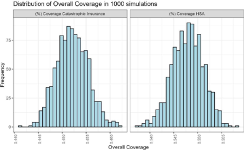
In Figure 3 we present the distributions of percentage of coverage for healthcare expenses, either by HSA or catastrophic insurance.

Figure 3
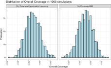
Distribution of percentage of coverage for healthcare expenses from HSA and catastrophic insurance in the 10,000,000 simulated individuals.

3.3 Savings account balance, coverage by HSA and coverage by catastrophic insurance

The proposed CDHP product has three main features: the HSA balance at 65 years-old, the expenses covered by the HSA and the expenses covered by catastrophic insurance. The first two features are more susceptible to the effects of a HSA on an individual behavior, as the decision to consume healthcare goods and services may be inhibited by this CDHP product. Table 4 displays descriptive statistics of these three features.

Table 4
Descriptive statistics of the HSA balance at 65 years-old, the expenses covered by the HSA and the expenses covered by catastrophic insurance over the work life. The percentiles, mean and standard deviation are calculated considering only the values greater than zero (n=10,000). We also present the mean (µ) and standard deviation (a) over the 1,000 simulations.

	HSA Balance		HSA Coverage		Cat, Insurance Coverage
	µ	σ	µ	σ	µ	σ
pctnul	0.73		0.00		5.59
p5	10,536	329	30,669	290	2,022	99
p10	16,737	300	35,956	263	4,281	145
p15	21,267	288	39,834	259	6,638	177
p25	28,263	271	45,996	249	11,970	249
p40	36,568	256	53,738	241	21,650	363
p50	41,535	248	58,645	248	29,666	459
p75	54,106	249	72,079	274	63,926	948
p85	60,242	257	79,243	298	94,228	1,586
p95	69,381	290	90,573	357	178,278	4,494
p98	74,616	342	96,831	359	264,692	6,711
max	89,251	1,355	100,000		1,176,242	119,167
mean	41,000	176	59,298	178	51,833	713
sd	17,739	108	18,015	111	69,719	2,297

• p(k): k-th sample percentile; SD: standard deviation.

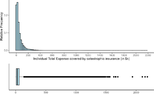
If a life did not have any expenses in the 40 years period, its account balance would be R$ 100,000, although the simulated mean and median balance at 65 years-old were between R$41,000 and R$41,535, in average with s.d. of R$248, and the maximum was R$ 89,251 in average, with s.d. of R$ 1,355. Therefore, the mean account balance at retirement is in average 42% the value which has been deposited. The mean expense covered during the work life by the insurance was around R$51,800, in average with s.d. of R$713, and the maximum was around R$1,176,000, in average with s.d. of R$ 119,167, which is 22 times the mean value, evidencing the presence of outliers. For 25% of the lives, the insurance covered lesser than R$ 12,000, and for half the lives it covered at most R$29,700 in average with s.d. of R$459. On the other hand, the 5% of lives with the greatest expenses covered by the insurance had more than R$ 175,000 covered in average. When considering the percentage of expenses covered by the insurance, half the lives had at most 40% of them covered by the insurance in average, while 25% of the lives had almost half of their expenses covered by it in average, and 5% of the lives had more than 75% of their expenses covered by the insurance in average.

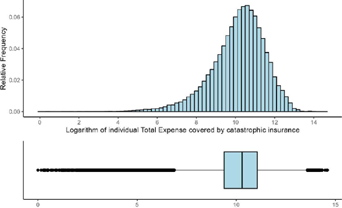
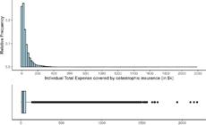
Figures 4 and 5 display the empirical distribution of the severity of catastrophic insurance use, and of its logarithm transformation, where it can be noted the presence of outliers, evidencing the coverage of great healthcare expenses by the insurance. Coverages under R$1.00 were ignored in the logarithmic transformation.

Figure 4
Severity of catastrophic insurance use in the 10,000,000 simulated individuals.

Figure 5
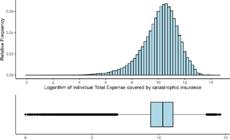
Logarithm transform of severity of catastrophic insurance usage in the 10,000,000 simulated individuals.

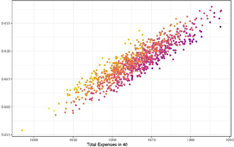
In Figure 6 we present the dispersion plot between the total expenses at the 40 year period of each life and the percentage of these expenses which were covered by catastrophic insurance. The color of the points refers to the number of times in which the insurance was used overthe work life.

Figure 6
Dispersion plot between the total expenses at the 40 year period of each life in the 10,000,000 simulated individuals and the percentage of these expenses which were covered by catastrophic insurance. The color refers to the number of times in which the insurance was used over the work life.

4. Discussion and Conclusions

An increase in healthcare costs has been observed recently in several countries, especially in Brazil, where it has led to a discussion about co-payment and deductible devices for health plans, which culminated in a resolution by the regulatory agency (ANS) to incorporate these devices to the Brazilian supplementary health system. A negative public repercussion based on misunderstandings followed the resolution, forcing ANS to revoke it, leaving the market uncovered regarding the understanding of these devices. In this context, this paper aimed to subsidize the discussion about co-payment and deductibles by simulating a consumer directed health plan product which has never been commercialized in Brazil, the health savings accounts, which combines a high deductible health plan with tax breaks to form a savings account aiming to reduce the individual exposition to the risk of extremal events by combining a catastrophic insurance with an individual savings account.

This mixed product benefits both the employer and employee. From the employee point of view, the accredited network of healthcare providers is superior than the standard, and the individual is not limited to the accredited network. Moreover, the balance may be invested to increase income, but due to the purpose of this work, this issue of investment has not been considered. From the employer point of view, it is expected lower individual healthcare expenses, since the employees, when paying for their own healthcare goods and services, tend to be more selective in choosing their providers and more thrifty when using the available services.

In order to carry out our simulation, we had to first establish a prediction technique for annual healthcare expenses. To address this challenge, we proposed an approach to healthcare expenses prediction based on Markov Chains, which seeks to predict the annual expenses of an individual based on his or her sex, age range and expenses in the last two years. In this approach, first the expense level is estimated and then, the exact expense is chosen from an empirical distribution.

Although classical in Statistics and Probability Theory, and applied in health economics to predict health conditions and costs related to it (Komorowski and Raffa (2016), Sato and Zouain (2010), Jeong et al. (2014), Graves et al. (2016), Bala and Mauskopf (2006), Dobi and Zempléni (2019) and Garg et al. (2010)), it seems that a Markov Chain approach may also be useful to predict annual healthcare expenses, as it is known that expenses history is an important factor in predicting healthcare expenses (Duncan et al., 2016). A Markov Chain approach based on previous expenses, sex, and age range may be more viable for pricing health plans than a method based on health condition due to ethical issues.

Based on a dataset containing annual expenses of a portfolio of a Brazilian self-management health plan, we simulated the proposed HSA product for 10,000 lives from 25 to 65 years-old in order to study the balance of the individual savings accounts over time and at retirement, and the frequency and severity of catastrophic insurance use. In this simulation, we took into account the persistence of costs phenomenon, widely known to be part of individual healthcare expenses. The results evidenced a low prevalence of persistence of costs at the individual level, as at 65 years-old the balance of the individual savings accounts is symmetrically spread around the average of R$ 44,000, supporting that the adoption of this model is not a mechanism of inequalities generation. During the 40 years period in the 10,000,000 simulated individuals, the total healthcare expenses of the simulated portfolio was R$1,082,350,725 in average with s.d. of R$7,688,268, of which R$489,367,594 in average (45.2%) with s.d. R$6,862,835 was covered by catastrophic insurance. From the individual perspective, half the lives had 40% of their expenses covered by catastrophic insurance and only 5% of them had more than 75% of their expenses covered by catastrophic insurance. At retirement, the mean balance of the individual accounts was 45.2% of the value deposited over the work life, so the mean expense covered by the HSA during the work life was 54.8% that deposited, in average.

Therefore, we may conclude that a mixed CDHP product combining a HSA and a catastrophic insurance may be viable in Brazil from a population point of view as it does not create inequalities caused by persistence of costs. In order to implement such a product, one needs to adapt the value deposited by the employer every year and the limit covered by the HSA to suit the health system costs.

We leave some topics for future research. An interesting topic would be to compare a Markov Chain approach to healthcare expenses prediction with the usual methods based on regression. Also, the development of a method which incorporates the best features of both approaches seems promising. About the proposed CDHP, there are some hyperparameters which can be optimized in order to obtain a more realistic simulation: the break points of the expense levels, the value deposited by the employer every year and the limit of expenses covered by the HSA. In order to optimize these quantities, it would be needed data with better quality and greater quantity than that of this paper. Finally, to further the discussion in Brazil about co-payment and deductible devices, it would be interesting to study other kinds of CDHP products in the Brazilian context.

Appendix A Descriptive Statistics and Transition Matrix

A.1 Descriptive Statistics of Annual Expenses, by sex

In this section, it is presented descriptive statistics by sex of the annual expenses individuals by sex, between 25 and 65 years-old which stayed on the portfolio during the whole five years period. The percentiles, mean and standard deviation are calculated considering only the individuals with positive expenses.

Table A.1
Descriptive Statistics Annual Expenses (Female)

Description	2005	2006	2007	2008	2009
n	13,539	13,539	13,539	13,539	13,539
PctNoExpense	5.09	5.26	5.16	5.15	5.55
p25	457	422	449	487	490
p50	998	940	987	1,130	1,104
p75	2,193	2,029	2,152	2,539	2,464
p90	4,808	4,462	4,848	5,603	5,453
p95	8,402	7,501	8,247	9,338	9,662
p96	9,781	8,818	9,393	10,659	11,122
p97	11,293	10,376	11,416	12,757	13,915
p98	14,425	13,252	15,886	17,114	19,095
p99	24,076	21,371	24,681	27,696	30,718
p995	33,027	34,656	44,429	51,048	53,649
p999	68,154	125,250	98,976	137,450	203,682
max	282,993	528,293	355,220	1,044,525	550,309
mean	2,341	2,327	2,494	2,956	3,062
sd	6,068	8,897	7,828	13,247	11,958

• n: total of individuals in portfolio; p(k): k-th sample percentile; sd: standard deviation.

Table A.2
Descriptive Statistics Annual Expenses (Male)

Description	2005	2006	2007	2008	2009
n	14,241	14,241	14,241	14,241	14,241
PctNoExpense	6.81	5.77	6.35	5.93	5.97
p25	237	231	252	289	271
p50	580	572	625	721	681
p75	1,351	1,336	1,432	1,677	1,594
p90	2,983	2,914	3,208	3,927	3,868
p95	5,588	5,491	6,259	7,680	8,212
p96	6,847	6,838	7,833	9,690	10,494
p97	8,799	8,865	10,461	12,985	14,589
p98	12,720	12,836	14,960	19,653	21,593
p99	22,163	21,840	26,596	34,427	36,397
p995	35,525	36,021	42,975	59,041	57,155
p999	100,317	100,298	90,679	139,391	146,580
max	426,772	371,231	266,119	286,716	965,287
mean	1,795	1,768	1,956	2,473	2,576
sd	7,490	7,306	7,235	9,786	13,316

• n: total of individuals in portfolio; p(k): k-th sample percentile; sd: standard deviation.

A.2 Descriptive statistics of annual expenses, by sex and age category

In this section, it is presented descriptive statistics by age range of the annual expenses of individuals between 25 and 65 years-old which stayed on the portfolio during the whole five years period. The percentiles, mean and standard deviation are calculated considering only the individuals with positive expenses.

Table A.3
Descriptive Statistics Annual Expenses (Female) 21a24

Description	2005	2006	2007	2008
n	555	372	210	75
PctNoExpense	1.98	3.76	5.24	9.33
p25	339	349	390	291
p50	833	730	888	699
p75	1,974	1,740	2,278	1,334
p90	4,661	3,678	5,621	3,088
p95	6,495	5,171	9,039	6,091
p96	7,803	6,268	11,516	6,626
p97	8,963	7,937	12,664	6,749
p98	10,295	10,176	19,717	8,433
p99	14,738	11,447	29,037	10,056
p995	19,713	15,185	30,401	10,823
p999	74,328	32,586	63,712	11,437
max	130,804	41,884	72,040	11,591
mean	2,030	1,617	2,609	1,410
sd	6,198	3,051	6,446	2,122

• n: total of individuals in portfolio; p(k): k-th sample percentile; sd: standard deviation.

Table A.4
Descriptive Statistics Annual Expenses (Male) 21a24

Description	2005	2006	2007	2008
n	375	250	149	65
PctNoExpense	10.93	12.00	14.77	15.38
p25	182	127	139	123
p50	415	322	366	296
p75	997	803	809	848
p90	2,338	1,710	2,080	1,682
p95	6,259	3,174	3,354	1,891
p96	8,641	3,473	4,105	1,938
p97	10,881	3,739	4,756	3,092
p98	13,469	4,524	8,094	4,712
p99	16,587	7,974	10,062	10,423
p995	25,255	20,678	10,517	13,634
p999	94,741	23,561	10,945	16,203
max	128,157	24,017	11,052	16,846
mean	1,688	889	923	899
sd	7,596	2,362	1,762	2,330

• n: total of individuals in portfolio; p(k): k-th sample percentile; sd: standard deviation.

Table A.5
Descriptive Statistics Annual Expenses (Female) 25a30

Description	2005	2006	2007	2008	2009
n	1,541	1,371	1,267	1,160	1,002
PctNoExpense	4.67	4.60	3.95	4.31	5.29
p25	393	328	330	372	358
p50	907	737	769	880	880
p75	2,427	1,751	1,797	2,011	1,873
p90	5,535	4,493	4,694	5,093	4,647
p95	8,885	8,096	7,014	8,777	9,509
p96	9,876	8,901	7,996	10,444	10,602
p97	10,801	10,246	8,702	11,730	12,047
p98	12,642	11,821	10,653	13,740	14,197
p99	17,993	17,090	14,164	18,273	19,864
p995	24,900	21,846	27,135	29,606	27,090
p999	52,313	38,304	83,367	74,171	42,511
max	85,433	52,910	118,517	80,355	57,494
mean	2,279	1,887	2,002	2,223	2,114
sd	4,416	3,656	5,623	5,058	4,204

• n: total of individuals in portfolio; p(k): k-th sample percentile; sd: standard deviation.

Table A.6
Descriptive Statistics Annual Expenses (Male) 25a30

Description	2005	2006	2007	2008	2009
n	1,243	1,072	915	793	681
PctNoExpense	7.48	7.74	8.09	10.47	11.01
p25	179	160	180	195	177
p50	406	379	433	450	416
p75	990	858	906	1,079	1,014
p90	2,192	1,927	1,802	2,349	2,500
p95	3,635	4,106	3,435	4,680	4,462
p96	4,197	5,306	3,999	6,085	5,243
p97	6,112	7,026	5,596	6,553	6,861
p98	9,181	9,000	7,460	11,110	10,335
p99	16,453	18,774	13,060	20,153	19,082
p995	26,250	21,917	19,561	35,258	54,969
p999	63,068	67,481	66,575	95,351	201,729
max	229,290	128,291	199,011	147,129	323,604
mean	1,388	1,290	1,255	1,578	2,038
sd	7,579	5,432	7,288	7,035	14,706

• n: total of individuals in portfolio; p(k): k-th sample percentile; sd: standard deviation.

Table A.7
Descriptive Statistics Annual Expenses (Female) 31a35

Description	2005	2006	2007	2008	2009
n	1,872	1,806	1,707	1,566	1,454
PctNoExpense	5.02	4.32	4.98	4.92	5.85
p25	368	335	393	373	341
p50	845	817	863	942	804
p75	1,948	1,884	1,909	2,245	1,877
p90	4,659	4,735	4,757	5,259	4,887
p95	8,907	7,946	8,319	9,141	8,771
p96	10,201	9,012	9,227	10,004	9,550
p97	11,406	9,878	10,565	10,924	10,444
p98	13,272	10,757	13,401	13,968	14,317
p99	17,819	15,736	20,232	18,703	19,230
p995	28,856	24,549	31,337	27,130	33,526
p999	59,213	64,758	70,975	71,472	52,075
max	87,084	101,389	98,995	141,717	69,533
mean	2,146	1,964	2,174	2,342	2,101
sd	4,815	4,583	5,234	5,756	4,532

• n: total of individuals in portfolio; p(k): k-th sample percentile; sd: standard deviation.

Table A.8
Descriptive Statistics Annual Expenses (Male) 31a35

Description	2005	2006	2007	2008	2009
n	1,908	1,801	1,664	1,462	1,248
PctNoExpense	7.39	6.89	8.17	7.25	7.05
p25	195	181	188	206	176
p50	460	436	475	527	483
p75	1,026	976	1,106	1,205	1,123
p90	2,010	2,044	2,342	2,862	2,561
p95	3,546	3,299	4,449	5,792	4,816
p96	4,413	3,778	5,336	8,042	6,489
p97	5,803	4,659	6,675	10,330	8,563
p98	8,308	7,118	9,835	12,979	12,292
p99	13,512	15,364	19,401	22,030	18,377
p995	22,473	21,891	25,576	42,934	21,802
p999	67,187	107,083	63,819	92,329	42,142
max	130,614	172,207	90,771	113,230	61,267
mean	1,243	1,295	1,357	1,792	1,396
sd	4,771	6,417	4,446	6,534	3,639

• n: total of individuals in portfolio; p(k): k-th sample percentile; sd: standard deviation.

Table A.9
Descriptive Statistics Annual Expenses (Female) 36a40

Description	2005	2006	2007	2008	2009
n	2,242	2,204	2,126	2,056	1,959
PctNoExpense	5.62	6.72	6.40	5.54	5.77
p25	363	344	346	379	390
p50	793	762	791	916	937
p75	1,871	1,628	1,802	2,141	2,053
p90	4,520	3,644	4,375	5,012	4,378
p95	8,043	6,276	7,735	8,502	8,314
p96	9,237	7,244	8,981	9,400	9,402
p97	10,519	8,840	10,607	10,728	10,757
p98	12,118	10,912	13,138	13,291	13,554
p99	18,267	15,634	20,821	21,374	19,857
p995	25,417	31,130	56,363	40,889	27,142
p999	75,004	102,143	85,783	176,175	113,373
max	157,006	528,293	92,919	318,932	221,151
mean	2,058	2,154	2,153	2,745	2,336
sd	5,657	13,605	6,006	12,851	8,471

• n: total of individuals in portfolio; p(k): k-th sample percentile; sd: standard deviation.

Table A.10
Descriptive Statistics Annual Expenses (Male) 36a40

Description	2005	2006	2007	2008	2009
n	2,286	2,195	2,139	2,088	2,052
PctNoExpense	7.09	6.33	6.69	6.90	7.26
p25	209	216	214	229	204
p50	513	496	500	553	512
p75	1,211	1,111	1,098	1,299	1,170
p90	2,682	2,424	2,386	2,679	2,744
p95	5,035	4,506	4,694	4,616	5,537
p96	6,375	5,409	5,287	5,164	6,540
p97	7,534	6,514	6,862	6,745	8,344
p98	10,579	9,115	9,601	9,955	11,419
p99	19,902	14,195	17,052	16,145	20,056
p995	24,752	21,963	34,069	22,558	31,768
p999	99,053	42,568	83,016	71,215	115,938
max	230,437	162,392	211,526	286,716	142,242
mean	1,564	1,327	1,535	1,558	1,635
sd	6,815	4,665	6,983	7,595	6,326

• n: total of individuals in portfolio; p(k): k-th sample percentile; sd: standard deviation

Table A.11
Descriptive Statistics Annual Expenses (Female) 41a45

Description	2005	2006	2007	2008	2009
n	2,557	2,494	2,454	2,382	2,339
PctNoExpense	6.14	6.01	5.30	5.58	6.67
p25	455	413	434	443	447
p50	949	859	912	985	977
p75	2,031	1,804	1,887	2,125	2,021
p90	4,369	3,735	4,018	4,842	4,648
p95	7,502	6,142	6,514	8,198	8,096
p96	8,718	7,183	7,572	9,834	9,821
p97	10,362	9,017	9,128	11,537	10,956
p98	13,856	11,100	12,013	14,644	13,852
p99	25,158	18,653	19,821	23,148	21,052
p995	34,825	30,076	28,599	35,298	50,353
p999	48,097	81,079	115,517	118,538	177,314
max	66,973	162,119	196,400	201,497	254,654
mean	2,140	1,993	2,188	2,503	2,563
sd	4,509	6,006	7,444	8,070	9,987

• n: total of individuals in portfolio; p(k): k-th sample percentile; sd: standard deviation.

Table A.12
Descriptive Statistics Annual Expenses (Male) 41a45

Description	2005	2006	2007	2008	2009
n	2,489	2,446	2,376	2,381	2,317
PctNoExpense	7.35	5.27	6.02	5.50	4.92
p25	233	225	230	270	246
p50	559	534	566	673	573
p75	1,312	1,272	1,280	1,498	1,306
p90	2,765	2,692	2,832	3,318	2,987
p95	4,860	5,530	5,428	6,306	6,220
p96	5,590	6,698	6,697	7,610	7,884
p97	7,162	8,705	8,475	9,842	9,736
p98	10,509	11,371	12,263	14,657	13,208
p99	17,289	16,961	19,340	25,622	24,125
p995	32,462	25,310	39,384	40,011	32,908
p999	91,013	54,602	71,849	94,264	75,851
max	117,357	267,607	244,532	140,615	114,218
mean	1,584	1,600	1,718	2,005	1,735
sd	5,447	6,817	7,229	7,051	5,285

• n: total of individuals in portfolio; p(k): k-th sample percentile; sd: standard deviation.

Table A.13
Descriptive Statistics Annual Expenses (Female) 46a50

Description	2005	2006	2007	2008	2009
n	2,337	2,440	2,464	2,520	2,531
PctNoExpense	4.45	5.00	5.24	5.40	5.33
p25	561	507	545	543	532
p50	1,131	1,058	1,121	1,234	1,133
p75	2,225	2,186	2,259	2,588	2,473
p90	4,625	4,572	4,471	5,128	5,336
p95	7,772	7,324	8,005	8,436	9,916
p96	9,564	8,366	9,267	9,812	12,467
p97	11,216	10,515	11,043	11,603	14,748
p98	14,077	13,077	14,062	15,898	17,793
p99	24,609	24,373	22,171	25,993	25,841
p995	27,863	37,853	35,379	55,079	45,159
p999	50,564	70,935	70,728	119,113	129,367
max	89,188	177,710	207,664	203,918	348,062
mean	2,296	2,322	2,434	2,795	2,946
sd	4,482	6,132	6,664	8,123	10,707

• n: total of individuals in portfolio; p(k): k-th sample percentile; sd: standard deviation.

Table A.14
Descriptive Statistics Annual Expenses (Male) 46a50

Description	2005	2006	2007	2008	2009
n	2,905	2,855	2,767	2,625	2,515
PctNoExpense	5.61	4.59	5.35	5.22	5.61
p25	263	257	281	299	281
p50	646	617	674	740	680
p75	1,439	1,440	1,477	1,661	1,525
p90	3,139	3,108	3,250	3,873	3,545
p95	5,968	5,723	6,672	7,680	8,102
p96	7,164	7,470	8,149	9,585	10,445
p97	9,182	9,022	11,134	15,316	15,606
p98	13,455	12,634	15,129	23,472	22,146
p99	20,150	23,003	27,865	37,801	45,070
p995	30,414	35,122	48,033	62,346	70,808
p999	98,447	86,831	89,023	113,012	160,275
max	426,772	137,333	124,276	275,813	397,015
mean	1,921	1,808	2,005	2,585	2,747
sd	9,858	5,929	6,495	10,411	13,107

• n: total of individuals in portfolio; p(k): k-th sample percentile; sd: standard deviation.

Table A.15
Descriptive Statistics Annual Expenses (Female) 51a55

Description	2005	2006	2007	2008	2009
n	1,491	1,646	1,847	2,031	2,204
PctNoExpense	4.63	3.65	4.44	4.38	4.95
p25	703	656	584	656	620
p50	1,394	1,265	1,207	1,388	1,337
p75	2,625	2,517	2,547	2,880	2,900
p90	5,317	5,024	5,686	6,299	6,104
p95	9,427	8,570	9,812	10,487	10,003
p96	11,851	10,229	11,274	12,000	12,111
p97	15,409	12,954	14,602	13,995	17,558
p98	20,293	19,269	19,709	21,897	27,194
p99	34,516	34,645	35,600	43,418	43,935
p995	56,503	78,735	55,339	53,830	75,109
p999	73,357	197,347	137,637	202,005	204,799
max	282,993	297,188	355,220	1,044,525	279,515
mean	3,130	3,355	3,188	3,859	3,680
sd	9,842	13,890	12,160	25,844	12,885

• n: total of individuals in portfolio; p(k): k-th sample percentile; sd: standard deviation.

Table A.16
Descriptive Statistics Annual Expenses (Male) 51a55

Description	2005	2006	2007	2008	2009
n	1,972	2,263	2,552	2,755	2,928
PctNoExpense	5.27	4.33	5.21	4.39	4.64
p25	314	312	330	391	345
p50	750	754	789	884	836
p75	1,642	1,658	1,785	1,963	1,874
p90	3,515	3,551	3,787	4,571	4,220
p95	6,266	6,527	7,079	8,413	9,370
p96	7,223	8,288	9,252	10,396	12,245
p97	10,201	10,694	13,255	13,862	15,997
p98	13,822	15,581	20,222	23,473	24,546
p99	31,181	25,131	32,155	39,463	36,614
p995	58,903	40,441	44,668	67,096	51,064
p999	109,224	100,505	90,346	157,042	171,368
max	112,453	371,231	129,112	267,595	965,287
mean	2,177	2,221	2,273	2,893	3,027
sd	7,391	10,533	6,786	11,132	20,648

• n: total of individuals in portfolio; p(k): k-th sample percentile; sd: standard deviation.

Table A.17
Descriptive Statistics Annual Expenses (Female) 56a60

Description	2005	2006	2007	2008	2009
n	831	980	1,098	1,211	1,309
PctNoExpense	6.26	6.33	5.19	4.54	3.97
p25	627	662	685	780	732
p50	1,366	1,346	1,432	1,615	1,648
p75	2,563	2,705	2,863	3,477	3,520
p90	5,487	6,278	5,818	6,573	7,741
p95	9,145	11,310	9,959	9,957	15,414
p96	11,318	13,667	11,264	11,932	19,931
p97	14,696	17,068	17,858	16,031	24,509
p98	19,522	20,310	23,083	19,755	29,453
p99	28,883	27,819	29,923	37,098	51,170
p995	56,251	40,600	40,949	43,065	94,078
p999	137,346	140,851	113,612	120,279	274,734
max	209,437	222,438	148,681	340,890	550,309
mean	3,157	3,258	3,175	3,659	4,931
sd	10,157	9,886	8,071	12,243	21,379

• n: total of individuals in portfolio; p(k): k-th sample percentile; sd: standard deviation.

Table A.18
Descriptive Statistics Annual Expenses (Male) 56a60

Description	2005	2006	2007	2008	2009
n	931	1,089	1,255	1,469	1,689
PctNoExpense	7.73	5.88	5.58	4.49	5.09
p25	377	353	421	457	442
p50	965	857	1,019	1,072	1,000
p75	2,293	1,995	2,353	2,415	2,381
p90	6,331	4,743	6,129	6,873	6,665
p95	13,567	10,440	12,530	12,824	15,095
p96	17,177	15,045	16,844	14,812	21,437
p97	20,182	19,150	20,385	19,038	26,588
p98	34,044	26,450	28,116	24,707	38,919
p99	42,818	40,854	43,186	39,265	57,110
p995	75,095	68,072	54,982	61,353	70,828
p999	98,802	108,815	106,887	132,189	165,958
max	105,272	168,989	144,749	153,098	201,089
mean	3,397	2,973	3,259	3,311	3,791
sd	9,557	9,741	8,983	9,333	11,983

• n: total of individuals in portfolio; p(k): k-th sample percentile; sd: standard deviation.

Table A.19
Descriptive Statistics Annual Expenses (Female) 61a65

Description	2005	2006	2007	2008	2009
n	113	226	366	538	741
PctNoExpense	3.54	6.64	5.19	6.69	6.48
p25	675	732	643	824	784
p50	1,250	1,415	1,509	1,803	1,732
p75	2,954	2,864	3,455	4,261	3,444
p90	6,080	5,454	8,467	9,869	7,437
p95	10,928	8,319	17,779	20,360	15,702
p96	11,122	11,551	20,114	25,948	19,334
p97	11,801	14,764	26,854	28,537	26,256
p98	12,380	16,414	33,172	37,319	30,266
p99	17,442	20,332	56,645	63,507	42,492
p995	19,103	44,430	60,399	71,529	126,540
p999	20,255	56,734	150,422	132,337	240,232
max	20,543	59,669	195,519	135,830	274,612
mean	2,603	2,898	4,505	5,116	4,905
sd	3,544	5,850	13,086	12,251	18,070

• n: total of individuals in portfolio; p(k): k-th sample percentile; sd: standard deviation.

Table A.20
Descriptive Statistics Annual Expenses (Male) 61a65

Description	2005	2006	2007	2008	2009
n	132	270	424	603	811
PctNoExpense	8.33	8.89	8.25	7.63	7.52
p25	361	313	411	539	480
p50	744	940	1,026	1,283	1,133
p75	2,198	2,243	2,449	3,129	2,733
p90	4,427	5,697	5,275	8,083	7,854
p95	7,887	14,443	11,139	25,074	19,228
p96	8,416	16,886	13,019	31,824	23,151
p97	8,923	18,602	15,341	41,806	28,318
p98	10,875	38,905	24,083	49,420	35,593
p99	20,273	49,467	29,582	107,065	90,216
p995	26,916	53,310	59,040	152,434	112,752
p999	32,392	106,560	197,939	229,425	229,212
max	33,761	123,830	266,119	237,957	320,963
mean	2,021	3,500	3,398	5,923	4,872
sd	4,053	10,600	14,966	20,614	18,301

• n: total of individuals in portfolio; p(k): k-th sample percentile; sd: standard deviation.

Figure A.1.
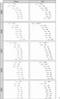
Profile plot of the mean annual expenses by year, for each sex and age range considering only individuals between 25 and 65 years-old which stayed on the portfolio during the whole five years period.

Figure A.2
Transition matrices of expenses for each two years combination, i.e. from 2005 to 2009, considering individuals with ages between (a) 21 to 40 years-old, and (b) 41 to 65 years-old.

Appendix B Markov Chains and HSA simulation

The Markov Chain approach proposed in this paper aims to predict the expense level of an individual in a given year by estimating the probability of his or her annual expenses being at every level given the expense level of previous years. Formally, considering the definition of F_j,i presented in Section 2.5.1, the probability of an individual with annual expenses in F_k,i·at year i having annual expenses in F_l,j at year j is estimated as:

(1) $\widehat{P}\left(F_{k,i},F_{l,j}\right)=\frac{\text{Number of individuals in }{F}_{k,i}\text{which are also in }{F}_{l,j}}{\text{Number of individuals in }{F}_{k,i}},\text{with}j>i.$

In Markov Chain Theory, $\widehat{P}\left(F_{k,i},F_{l,j}\right)$ is an estimator of the transition probabilities between states F_k,i· and F_l,j. Indeed, the ratio above is the proportion of individuals which were in F_k,i· at year i and transitioned to F_l,j at year j. Therefore, if we were to estimate the probability of an individual in F_k,i· to be in F_l,j at year j we could use the proportion $\widehat{P}\left(F_{k,i},F_{l,j}\right)$, which is a consistent estimator for such probability (Anderson and Goodman, 1957).

The approach above may also be applied to estimate the transition probabilities for individuals of a given sex and/or age range. This probability would allow to study the persistence of costs in distinct groups of individuals, as it is believed to behaviour differently for each age range and sex. The estimation of these probabilities would be done in the same manner as above, but the number of individuals considered in the ratio of $\widehat{P}\left(F_{k,i},F_{l,j}\right)$ would be that within the group of interest. Proceeding this way, we have a prediction for the probability of an individual, with given sex, age range and expense level in a previous year, to be in each expense level in the current year.

A transition matrix characterizes a Markov Chain, that is a sequence of random variables in which the distribution of the current random variable depends only on the value of the previous k and is given by the probabilities of the transition matrix, in which k is called the order of the Markov Chain. If k = 1 then the transition matrix is calculated as the ratio given in (1) when j = i+1. If k = 2, then the probability of being in a given state after visiting some in the past depends only on the last two states visited. In this case, the Markov Chain is generated by the transition probabilities estimated as which refers to the transition to F_l,i after being in F_k,i−2, F_m,i−1 at the previous two years. These probabilities may also be estimated for a given group of individuals, considering the numbers in the ratio to be that within the group.

(2) $\widehat{P}\left(F_{k,i-2},F_{m,i-1};F_{l,i}\right)=\frac{\text{Number of individuals in }{F}_{k,i-2}\text{which are also in }{F}_{m,i-1}\text{and}{F}_{l,i}}{\text{Number of individuals in }{F}_{k,i-2}\text{which are also in}{F}_{m,i-1}}$

With a Markov Chain of order 2 we may estimate the probability of an individual with given sex and age range to be in each expense level as a function of the levels he or she was in the last two years. This is the method we use to predict the expense level of each life in the simulated portfolio. Observe that it diverges from the usual methods based on regression as we do not try to predict the exact value of the annual expense, but rather the expense level, so we do not have to assume a distribution for the expenses, nor a functional relation between the current year expenses and the independent variables sex, age range and previous two years expenses.

Transition Matrices: In order to perform the first step of the simulation, we need to estimate a transition matrix between the expense levels. For this purpose, we suppose that the expense level follows a homogeneous Markov Chain of order 2 (Taylor and Karlin, 1998). This means the transition from one state to another does not depend on the year, but only on the states. Formally, this means that

(3) $P\left(F_{k,i-2},F_{m,i-1};F_{l,i}\right)=P\left(F_{k,j-2},F_{m,j-1};F_{l,j}\right)$

for any i, j, in which P is the population transition probability, in contrast to the estimated transition probability P̂. With this assumption, we may estimate the transition probabilities by that of the time period 2007 to 2009. Therefore, we estimate the transition from expense levels F_k, F_m to F_i as

(4) $\widehat{P}\left(F_k,F_m;F_l\right)=\widehat{P}\left(F_{k,2007},F_{m,2008};F_{l,2009}\right),$

in which we consider only the individuals within the respective sex and age range group in the ratios that define these transitions. This assumption is supported by the matrices in Figure 1, where we see that those which compare years with the same distance are similar (these are the matrices in a same diagonal of Figure 1).

Under this approach, we have 16 transition matrices, one for each combination of sex and age range (26-30, 31-35, 36-40, 41-45, 46-50, 51-55, 56-60, 61-65). Each matrix has 16 rows, one for each pair of expense levels in the current and last year, and 4 columns, one for each possible expense level in the next year. The entries of these matrices are transition probabilities from the state given by the pair to each one of the expense levels. To estimate the transitions, we consider that the age range of each individual in the dataset is the one which he or she was part of for the most number of months in the triennial 2007-2009.

First step The expense level of an individual next year is predicted based on his or her sex, age range and expense level last year and in the current year. This prediction is sampled from the estimated conditional distribution of the expense levels of given sex, age range and two last expense levels, which is the row associated to the last two expense levels of the transition matrix of the given sex and age range. We start this process at the initial values for 24 and 25 years-old to estimate the level at 26 years-old. We then iterate this process to estimate the level for the following ages: use the estimated values for 25 and 26 to predict 27 years-old; that of 26 and 27 to predict 28 years-old, and so on until the age of 65. Therefore, for each one of the 10,000 lives, we have a sequence of 41 levels corresponding to its predicted expense level for each work life year. Observe that, from age 27 on, the expenses history is predicted in the previous two years.

Second step After we simulate the expense level of a life in a given year, we need to simulate the value to be withdrawn from its account to cover a healthcare expense in such level. This is done by sampling a point from the empirical distribution of the aggregated annual expenses of all years which contain only the individuals with the same sex and age range of the life. Within this empirical distribution, we sample one of the points inside the expense level predicted on step one, i.e., inside the respective dotted lines in Figure B.1, which shows the aggregated empirical distributions of the logarithm of the annual healthcare expenses between 2005 and 2009 for each sex and age range.

In Table B.1 we see the number of expenses in the dataset at each expense level by sex and age range. These percentages aggregate all expenses of the period, so they refer to the percentage of expenses, rather than the percentage of individuals, as each individual has five expenses, one for each year. In the dataset, 25% of women’s expenses and 45% of men’s in the age range 25-30 are in the first level (up to R$ 300), percentages which decrease with age, attaining the values of 15% and 23% for women’s and men’s, respectively, at the age range 61-65. As the age increases, the same reduction is observed in the percentage of expenses in the second expense level (R$ 300 - R$ 1,000) for both sexes. On the other hand, the percentage ofexpenses in the third expense level (R$ 1,000 - R$ 5,000) increases with age and the difference between these percentages in age ranges 25-30 and 61-65 is 14 and 17 percentage points for women’s and men’s, respectively. The same is observed for the fourth expense level (greater than R$ 5,000): 10% of women’s expenses and 4% of men’s in the age range 25-30 are greater than R$ 5,000 in opposition to 16% of women’s and 12% of men’s in the age range 61-65. We see in the last three age ranges (after 51 years-old) that around 58% to 62% of women’s expenses, and 40% to 48% of men’s, are greater than R$ 1,000.

Table B.1.
Percentage of expenses in each expense level by sex and age range. The expenses of all years are aggregated, so these percentages refer to the percentage of expenses, rather than the percentage of individuals, as each individual has five expenses, one for each year.

Age Range	Female				Male
	[0-300]	(300-1000]	(1000-5000]	>5000	[0-300]	(300-1000]	(1000-5000]	>5000
25a30	1,597 (25.2%)	2,071 (32.7%)	2,076 (32.7%)	597 (9.4%)	2,138 (45.5%)	1,531 (32.5%)	861 (18.3%)	174 (3.7%)
31a35	2,091 (24.9%)	2,741 (32.6%)	2,790 (33.2%)	783 (9.3%)	3,374 (41.7%)	2,690 (33.3%)	1,703 (21.1%)	316 (3.9%)
36a40	2,678 (25.3%)	3,581 (33.8%)	3,485 (32.9%)	843 (8.0%)	4,121 (38.3%)	3,683 (34.2%)	2,473 (23.0%)	483 (4.5%)
41a45	2,633 (21.5%)	4,133 (33.8%)	4,522 (37.0%)	938 (7.7%)	4,153 (34.6%)	4,134 (34.4%)	3,080 (25.6%)	642 (5.3%)
46a50	2,198 (17.9%)	3,765 (30.6%)	5,194 (42.3%)	1,135 (9.2%)	4,201 (30.7%)	4,703 (34.4%)	3,892 (28.5%)	871 (6.4%)
51a55	1,354 (14.7%)	2,545 (27.6%)	4,258 (46.2%)	1,062 (11.5%)	3,265 (26.2%)	4,117 (33.0%)	4,166 (33.4%)	922 (7.4%)
56a60	818 (15.1%)	1,313 (24.2%)	2,591 (47.7%)	707 (13.0%)	1,527 (23.7%)	1,877 (29.2%)	2,315 (36.0%)	714 (11.1%)
61a65	309 (15.6%)	442 (22.3%)	917 (46.2%)	316 (15.9%)	524 (23.4%)	646 (28.8%)	796 (35.5%)	274 (12.2%)

Figure B.1
Empirical distributions of the logarithm of the annual healthcare expenses between 2005 and 2009. The distributions aggregate points from the five years. The dotted lines are respectively log(300), log(1000) and log(5000), which are the break points of the expense levels F_i,j.

Bibliography

• Anderson, T. W. and L. A. Goodman (1957): “Statistical Inference about Markov Chains”, Ann. Math. Statist, 1 (28), 89–110. [34]
• ANS (2019-2021a): “Dados Gerais - ANS,” Website, Agência Nacional De Saúde Suplementar, acessed on October 9th, 2019. [2]
• ANS (2019-2021b): “Mapa Estratégico 2019-2021 - ANS,” Website, Agência Nacional De Saúde Suplementar, acessed on October 9th, 2019. [2]
• Bala, M. V. and J. A. Mauskopf (2006): “Optimal assignment of treatments to health states using a Markov decision model”, PharmacoEconomics, 4 (24), 345–354. [17]
• Bundorf, M. K. (2016): “Consumer-directed health plans: A review of the evidence”, The Journal Risk and Insurance, 83 (1), 9–41. [1, 2]
• Dobi, B. and A. Zempléni (2019): “Markov chain-based cost-optimal control charts for healthcare data,” Preprint 1903.06675, arXiv, acessed on October 9th, 2019. [17]
• Duncan, I., M. Loginov, and M. Ludkovski (2016): “Testing alternative regression frameworks for predictive modeling of health care costs”, North American Actuarial Journal, 1 (20), 65–87. [5, 8, 17]
• Ehrlich, I. and G. S. Becker (1972): “Market insurance”, American Economic Review, 4 (80), 623–648. [2]
• Eichner, M., M. McClellan, and D. Wise (1996): “Insurance or self-insurance?: Variation, persistence, and individual health accounts,” Working Paper Series 5640, National Bureau of Economic Research. [7]
• Eichner, M. J. (1998): “The demand for medical care: What people pay does matter”, American Economic Review, 2 (88), 117–121. [2]
• Frees, E. W, R. A Derrig, and G. Meyers (2014): Predictive modeling applications in actuarial science, vol. 1, Cambridge University Press. [5]
• Frees, E. W, J. Gao, and M. A. Rosenberg (2011): “Predicting the frequency and amount of health care expenditures”, North American Actuarial Journal, 3 (15), 377–392. [8]
• Gabel, J. R., A. T. Lo Sasso, and T. Rice (2002): “Consumer-driven health plans: Are they more than talk now?” Health Affairs, 21 ((Suppl1)), W395–W407. [1]
• Garg, L., S. McClean, B. Meenan, and P. Millard (2010): “A non-homogeneous discrete time Markov model for admission scheduling and resource planning in a cost or capacity constrained healthcare system”, Health Care Manag Sci, 2 (13), 155–169. [17]
• Graves, N, C Wloch, J Wilson, A Barnett, A Sutton, N Cooper, K Merollini, V McCreanor, Q Cheng, E Burn, T Lamagni, and A. Charlett (2016): “A cost-effectiveness modelling study of strategies to reduce risk of infection following primary hip replacement based on a systematic review”, Health Technology Assessment, 54 (20), 1–144. [17]
• Jeong, S., C-H. Youn, and Y-W. Kim (2014): “Predicted cost model for integrated healthcare systems using Markov process,” in Ubiquitous Information Technologies and Applications, Springer, Berlin, Heidelberg, vol. 280 of Lecture Notes in Electrical Engineering, 181–187. [17]
• Jones, A. (2000): “Health Econometrics”, Handbook of Health Economics, 265–344. [3, 8]
• Komorowski, M. and J. Raffa (2016): “Markov Models and Cost Effectiveness Analysis: Applications in Medical Research”, Secondary Analysis of Electronic Health Records, 351–367. [17]
• Marcondes, D., C. P. Peixoto, and A. C. Maia (2018): “A survey of a hurdle model for heavy-tailed data based on the generalized lambda distribution”, Communications in Statistics - Theory and Methods. [9]
• Pope, G. C, J. Kautter, R. P Ellis, A. S Ash, J. Z Ayanian, L. I Lezzoni, M. J Ingber, J. M Levy, and J. Robst (2004): “Risk adjustment of Medicare capitation payments using the CMS-HCC model”, Health Care Financing Review, 4 (25), 119–141. [8]
• Sato, R. C. and D. M. Zouain (2010): “Markov models in health care”, Einstein (São Paulo), 3 (8), 376–379. [17]
• Seshamani, M. and A. Gray (2004): “Time to death and health expenditure: An improved model for the impact of demographic change on health care costs”, Age and Ageing, 6 (33), 556–561. [4]
• Taylor, H. M and S. Karlin (1998): An Introduction to Stochastic Modeling, Academic Press Limited., 3 ed. [3, 35]
• Werblow, A., S. Felder, and P. Zweifel (2007): “Population ageing and health care expenditure: A school of “red herrings”?” Health Economics, 10 (16), 1109–1126. [4]
• Yamamoto, D. H. (2013): “Health care costs - from birth to death,” Health Care Cost Institute’s Independent Report Series 2013-1, Society of Actuaries, acessed on October 1st, 2019. [5]
• Zweifel, P., S. Felder, and A. Werblow (2004): “Population ageing and health care expenditure: New evidence on the “red herring””, The Geneva Papers on Risk and Insurance, 4 (29), 652–666. [4]
• Zweifel, P. and W. G. Manning (2000): Moral hazard and consumer incentives in health care, Elsevier. [2]

Datas de Publicação

• Publicação nesta coleção
  19 Set 2025
• Data do Fascículo
  2025