THE TIGHTNESS OF STRENGTHENED SEMIDEFINITE RELAXATIONS FOR THE BOOLEAN QUADRATIC PROGRAMMING PROBLEM WITH GENERALIZED UPPER BOUND CONSTRAINTS

ABSTRACT

This paper studies semidefinite programming (SDP) relaxations for the Boolean Quadratic Programming problem with Generalized Upper Bound constraints (BQP-GUB), which arises in several application domains. We show that conventional semidefinite relaxation (SDR) does not yield tight bounds for this problem. We then analyze strengthened SDP relaxations and identify formulations that produce tight or near-tight bounds, particularly those based on reduced reformulation-linearization techniques (SDR+RRLT and SSDR+RRLT. Numerical experiments demonstrate that these approaches significantly reduce the relaxation gap compared to SDR, while highlighting the trade-off between bound quality and computational scalability.

Keywords:
BQP-GUB; SDP; semidefinite relaxation; vector lifting; matrix lifting; combinatorial optimization; enhanced semidefinite relaxation

1 INTRODUCTION

Consider S = {1, 2, . . . , n}, a finite set representing the first n natural numbers. Let p _i denote the cost associated with each i ∈ S, and r _ij denote the cost associated with each pair (i, j) ∈ S ×S. The linear vector p ^⊤ = (p ₁ , p ₂ , · · · , p _n ) represents the cost vector, while the matrix R = [r _{i j} ] ∈ ℝ^n×n represents the quadratic cost matrix. Without loss of generality, we assume that R is symmetric, since any asymmetric matrix can be replaced by $\frac{1}{2}(R+R^{\top })$ without affecting the objective value or the optimal solution set.

Let C ₁ ,C ₂ , . . . ,C _m be mutually disjoint subsets of S such that $S={\cup }_{k=1}^m{C}_k$. The Boolean Quadratic Programming problem with Generalized Upper Bound constraints (BQP-GUB) (Wang & Punnen, 2017) is given by:

$$\begin{gathered} \max f\left(x\right)=\sum _{i=1}^n{p}_i{x}_i+\sum _{i=1}^n\sum _{j=1}^n{r}_{ij}{x}_i{x}_j \\ \text{s.t.}\sum _{j\in C_k}{x}_j=1,k=1,2,\dots ,m, \\ {x}_j\in \{0,1\},j=1,2,\dots ,n. \end{gathered}$$ (1)

The above formulation represents a combinatorial optimization problem. The BQP-GUB problem generalizes the classical quadratic semi-assignment problem (QSAP).

QSAP has a wide range of applications, including co-clustering of image segments (Vitaladevuni & Basri, 2010), correlation clustering (Demaine et al., 2006), scheduling (Chrétienne, 1989), asset allocation (Gelenbe et al., 2010), and metric labeling (Kleinberg & Tardos, 2002). Consequently, BQP-GUB inherits significant practical relevance. The QSAP was first introduced by Greenberg (Greenberg, 1969), and has since been studied extensively in various contexts.

From a computational perspective, QSAP is a relaxation of the quadratic assignment problem (QAP), obtained by replacing assignment constraints with semi-assignment constraints. Since QAP is NP-hard, QSAP and BQP-GUB are also NP-hard (Chhajed & Lowe, 1992). Moreover, even moderate problem sizes are challenging; for example, QAP instances with dimension greater than 25 are already considered large-scale (Ding & Wolkowicz, 2009). Semidefinite programming (SDP) relaxations have been successfully applied to QAP, starting with the work of Zhao et al. (1998).

To address the computational difficulty of BQP-GUB, relaxation techniques are essential. While spectral methods are computationally attractive, they often produce weak bounds (Guattery & Miller, 1998; Kannan et al., 2004; Lang, 2005). In contrast, semidefinite relaxation (SDR) methods typically provide tighter bounds and have proven effective in various applications, including image segmentation (Heiler et al., 2005), co-segmentation (Joulin et al., 2010), and subgraph matching (Schellewald & Schnörr, 2005). However, a systematic and detailed study of SDP relaxations for BQP-GUB is still lacking.

Although SDR, redundant quadratic constraints, and reformulation-linearization techniques are well established, their structured application and comparative analysis for BQP-GUB remain largely unexplored. In this work, we address this gap by developing and analyzing several SDP-based relaxations tailored to the structure of BQP-GUB.

A key contribution of this paper is a unified theoretical and computational investigation showing that several seemingly different formulations are, in fact, equivalent in terms of bound quality. In particular, we demonstrate that improvements in relaxation strength primarily arise from the incorporation of stronger valid constraints, especially reduced reformulation linearization techniques (RRLT), rather than from alternative lifting strategies. This allows us to distinguish clearly between redundant formulations and those that provide meaningful improvements.

In addition, we propose an alternative enhanced semidefinite relaxation (AESDR) and evaluate its performance alongside existing methods. Extensive computational experiments on standard BQP-GUB instances highlight the trade-off between relaxation tightness and computational scalability: RRLT based formulations yield tighter bounds but are less scalable, whereas simpler relaxations remain computationally efficient for larger instances.

The main contributions of this work are summarized as follows:

• We provide a systematic study of SDP relaxations for the BQP-GUB problem, emphasizing structural properties that influence their performance;

• We establish theoretical equivalences among several formulations, showing that SDR, VSDR, and MSDR yield identical bounds, as do SSDR and ESDR, thereby reducing redundancy;

• We demonstrate that the primary improvement in relaxation quality is driven by RRLT constraints rather than alternative SDP formulations;

• We propose an alternative enhanced SDP relaxation (AESDR) and compare it with existing approaches;

• We present extensive numerical experiments (up to dimension 500) illustrating the trade-off between bound quality and computational scalability.

In the first Section, we introduce the problem, and in subsequent sections, we propose different semidefinite relaxations to this problem. In Section 10, we apply these methods to BQP-GUB datasets which we generated ourselves.

1.1 Notation

The following notations are used in this research.

1. X ⪰ 0: Symmetric matrix X is positive semidefinite and X ⪰ Y to denote X − Y is positive semidefinite.

2. X •Y: For n × n matrices X and Y , X •Y = tr(X ^⊤ Y).

3. diag(X ): The vector x with x _i = X _ii , i = 1, ..., n, where the matrix X is of size n × n.

4. trace(·): trace of a matrix

2 SEMIDEFINITE RELAXATION OF BQP-GUB (SDR)

BQP-GUB is known to be NP-hard. This means that no efficient exact algorithm is available. Since BQP-GUB is non-convex, it is difficult to solve using standard optimization methods.

A common approach to handle such problems is semidefinite relaxation (SDR). This method converts the non-convex problem into a convex one by relaxing certain constraints. However, SDR is often limited in practice because it requires high computational effort and usually gives weak bounds.

In this paper, we do not focus on reducing complexity. Instead, our goal is to develop a semidefinite relaxation that gives tighter bounds for BQP-GUB. In order to obtain the semidefinite relaxation and for ease of presentation, the objective function in 1 can be written in compact matrix-vector form as:

$$\begin{gathered} \max f\left(x\right)=p^{\top }x+x^{\top }Rx \\ \text{s.t.}\sum _{j\in C_k}{x}_j=1\text{for}k=1,2,\dots ,m, \\ {x}_j\in \{0,1\}\text{for}j=1,2,\dots ,n. \end{gathered}$$ (2)

where p ^⊤ = (p ₁ , p ₂ , ..., p _n ) and R = [r _{i j} ]_n×n . Since x _j ∈ {0, 1} for j = 1, 2, . . . , n, the linear term of the objective function can be replaced by a quadratic term, resulting in the following transformed problem formulation:

$$\begin{gathered} \max f\left(x\right)=x^{\top }Qx \\ \text{s.t.}\sum _{j\in C_k}{x}_j=1\text{for}k=1,2,\dots ,m, \\ {x}_j\in \{0,1\}\text{for}j=1,2,\dots ,n. \end{gathered}$$ (3)

where Q = [q _{i j} ] ∀i, j ∈ 1, 2, ..., n such that

$\left\{\begin{array}{l}{p}_i+r_{ij}\text{if}i=j,\\ r_{ij}\text{otherwise}.\end{array}\right.$

The optimal solution of the problem (3) is equal to the negative of the optimal solution of the following minimization problem:

$$\begin{gathered} minf\left(x\right)=x^{\top }\overline{Q}x \\ \text{s.t.}\sum _{j\in C_k}{x}_j=1\text{for}k=1,2,\dots ,m, \\ {x}_j\in \{0,1\}\text{for}j=1,2,\dots ,n. \end{gathered}$$ (4)

where $\overline{Q}=-Q$. Here, we consider the equivalent minimization form and for consistency, all subsequent SDP formulations are written using $\overline{Q}$.

In this paper, we propose some different SDP formulations of BQP-GUB 3. We begin with the first formulation as follows.

Since $x^{\top }\overline{Q}x=tr\left(\overline{Q}x{x}^{\top }\right)$, we introduce a matrix variable X = xx ^⊤. The condition X = xx ^⊤ is equivalent to requiring X ⪰ 0 and rank(X ) = 1. In semidefinite relaxation, the rank condition is dropped, yielding a convex feasible set.

For Boolean variables x _j ∈ {0, 1}, we have the identity $x_j^2=x_j$. Hence, the generalized upper bound constraints

$\sum _{j\in C_k}{x}_j=1,k=1,2,\dots ,m,$

can equivalently be written as

$\sum _{j\in C_k}{x}_j^2=1,k=1,2,\dots ,m,$

Let us define a matrix (D _k )_n×n = [(d _k )_ij ]_n×n such that

$(d_k{)}_{ij}=\left\{\begin{array}{l}1\text{for}i=j\in C_k\text{for}k=1,2,\dots ,m,\\ 0\text{otherwise}\end{array}\right.$

Therefore, the quadratic form of it is expressed as

$x^{\top }{D}_{k}x=1,k=1,2,\dots ,m.$

Finally, in terms of X, the constraints x ^⊤ D _k x = 1 can be represented as

$D_k\bullet X=1,k=1,2,\dots ,m,$

and the relation diag(X) = x is imposed to link X and x.

By lifting the vector variable x to the matrix variable X and applying the Schur complement (Boyd & Vandenberghe, 2004), the nonconvex constraint X = xx ^⊤ can be equivalently reformulated as

$\left[\begin{array}{cc}1& x^{\top }\\ x& X\end{array}\right]⪰0,\text{rank}\left(X\right)=1.$

The rank constraint is inherently nonconvex, which makes the problem computationally challenging. A common relaxation strategy is to omit the rank condition, thereby obtaining a convex semidefinite program (SDP). Alternative formulations introduce convex surrogates for the rank, such as Frobenius norm or nuclear norm penalties (see Nayak & Mohanty (2019)). In this work, we adopt the standard relaxation by simply dropping the rank constraint. The resulting semidefinite relaxation of the BQP-GUB (4) is

$$\begin{gathered} \min \overline{Q}\bullet X \\ \text{s.t.}{D}_k\bullet X=1,k=1,2,\dots ,m, \\ diag\left(X\right)=x, \\ \left[\begin{array}{cc}1& x^{\top }\\ x& X\end{array}\right]⪰0. \end{gathered}$$ (6)

Next, under additional assumptions, we obtain a relationship between optimal values between the problems (4) and (6).

Note that throughout the paper $p_1^{*}$ denotes the optimal value of the problem (4).

Theorem 1. If the problem (4) is feasible then the problem (6) is also feasible. If $p_2^{*}$ is the optimal value of the problem (6) then $p_1^{*}\ge p_2^{*}$ .

Proof. For feasible x to (4), set X = xx ^⊤. Then D _k • X = x ^⊤ D _k x = 1, diag(X ) = x, and $\left[\begin{array}{cc}1& x^{\top }\\ x& X\end{array}\right]⪰0$ with objective $Q\bullet X=x^{\top }Qx\ge p_2^{*}$, yielding $p_1^{*}\ge p_2^{*}$. □

The semidefinite relaxation (SDR) provides a convex approximation of the BQP-GUB problem, but it often produces loose bounds due to the relaxation of the rank and Boolean constraints. To improve the quality of the solution, it is useful to incorporate additional constraints that strengthen the SDP formulation. In the following section, we introduce a strengthened semidefinite relaxation (SSDR) that incorporates such constraints to achieve better approximate the original problem.

3 STRENGTHENED SEMIDEFINITE RELAXATION (SSDR) FOR BQP-GUB

To proceed with the second formulation, we define an m × n matrix A = [a _ij ] representing the generalized upper bound constraints, where

$a_{ij}=\left\{\begin{array}{l}1\text{if}j\in C_k\text{and}i=k,\\ 0\text{otherwise}.\end{array}\right.$

Let e ∈ ℝ^m denote the all-ones vector. Using this notation, the equality constraints of problem ((4)) can be written compactly as

$$\begin{gathered} \min f\left(x\right)=x^{\top }\overline{Q}x \\ \text{s.t.}Ax=e, \\ {x}_j\in \{0,1\},j=1,2,\dots ,n. \end{gathered}$$ (7)

which shows the equivalence of the problems (4) and (7).

A standard technique for improving relaxations is the addition of redundant constraints. Such constraints do not change the feasible set but can reduce the duality gap and yield tighter bounds. As shown in Anstreicher et al. (1999) and Anstreicher & Wolkowicz (2000), they may also help guarantee strong duality in situations where it would otherwise fail.

To strengthen (7), we include the squared-norm constraint

$\Vert Ax-e{\Vert }^2=0,$

which expands to (Ax − e)^⊤(Ax − e) = x ^⊤ A ^⊤ Ax − 2e ^⊤ Ax + e ^⊤ e. Since Ax = e is already enforced, this reduces to

$x^{\top }{A}^{\top }Ax=e^{\top }e.$

The resulting problem is a quadratically constrained quadratic program (QCQP):

$$\begin{gathered} \min x^{\top }\overline{Q}x \\ \text{s.t.}Ax=e, \\ {x}^{\top }{A}^{\top }Ax=e^{\top }e, \\ {x}_j\in \{0,1\},j=1,2,\dots ,n. \end{gathered}$$ (8)

The semidefinite relaxation (SDR) of this strengthened formulation is

$$\begin{gathered} \min \overline{Q}\bullet X \\ \text{s.t.}Ax=e, \\ diag\left(X\right)=x, \\ {A}^{\top }A\bullet X=e^{\top }e, \\ \left[\begin{array}{cc}1& x^{\top }\\ x& X\end{array}\right]⪰0. \end{gathered}$$ (9)

To improve the solution quality, stronger relaxations are needed. One effective approach is to incorporate reformulation-linearization techniques (RLT), which introduce additional inequalities and quadratic constraints. These strengthened relaxations tighten the feasible region and enhance the bounds. In the next section, we introduce RLT-based semidefinite relaxations and discuss their formulation and properties.

4 REFORMULATION LINEARIZATION TECHNIQUES BASED RELAXATIONS OF BQP-GUB

This section introduces semidefinite relaxations of BQP-GUB using the reformulation linearization techniques (RLT). For ease of presentation, we first define the relaxation gap and tightness of a semidefinite relaxation as follows.

Definition 1. The difference between the optimal solution of the original problem and the solution obtained using semidefinite relaxation is called the relaxation gap.

Definition 2.A tight relaxation in the context of semidefinite programming (SDP) refers to a specific type of relaxation where the optimal value of the relaxed problem (SDP) coincides with the optimal value of the original problem. This essentially means that the relaxed problem provides the exact solution to the original problem. In semidefinite programming (SDP), achieving a tight relaxation where the solution matches the original problem is often difficult and not guaranteed for all problems. Researchers and practitioners investigate conditions and methods to enhance the likelihood of achieving tight relaxation in specific problem classes. The proposed method outperforms the semidefinite relaxation method discussed in Section 2.

The problem (4) can be further strengthened by introducing additional quadratic constraints, as observed in prior literature (Anstreicher, 2009; Faye & Roupin, 2007). Here, we specifically investigate the incorporation of squared norm constraints and simple RLT inequalities (Sherali & Adams, 2013) in particular.

4.1 SSDR relaxation with RLT (SSDR+RLT)

If we add the RLT inequalities (Sherali & Adams, 2013)

$X_{ij}\ge 0,X_{ij}\ge x_i+x_j-1\forall i<j,$

and

$X_{ij}\le x_i\forall i\ne j,$

to problem (8), then it can be reformulated as

$$\begin{gathered} \min x^{\top }\overline{Q}x \\ \text{s.t.}Ax=e \\ {x}^{\top }{A}^{\top }Ax=e^{\top }e \\ {x}_i{x}_j\ge 0,x_i{x}_j\ge x_i+x_j-1\forall i<j \\ {x}_i{x}_j\le x_i\forall i\ne j \\ {x}_j\in \{0,1\},j=1,2,\dots ,n. \end{gathered}$$ (10)

Note that the inequality x _i x _j ≤ x _j is redundant, since it is obtained by interchanging the indices in x _i x _j ≤ x _i when the constraint is imposed for all ordered pairs i ≠ j.

The semidefinite relaxation of problem (10) is given by

$$\begin{gathered} \min \overline{Q}\bullet X \\ \text{s.t.}Ax=e \\ \mathrm{diag}\left(X\right)=x \\ {A}^{\top }A\bullet X=e^{\top }e \\ {X}_{ij}\ge 0,X_{ij}\ge x_i+x_j-1\forall i<j \\ {X}_{ij}\le x_i\forall i\ne j \\ \left[\begin{array}{cc}1& x^{\top }\\ x& X\end{array}\right]⪰0. \end{gathered}$$ (11)

Now to understand the effectiveness of SSDR+RLT in (11), we start comparing the optimal values of (7) and (11). As the problems (4) and (7) are same, therefore, $p_1^{*}$ is also optimal value of the problem (7). Then, assuming further conditions, we demonstrate the relation between the optimal values and solutions for (7) and (11).

Theorem 2. If the problem (7) is feasible then the problem (11) is also feasible. If $p_3^{*}$ is the optimal value of the problem (11) then $p_1^{*}\ge p_3^{*}$ .

Proof. Let x ∈ ℝⁿ solve (7) feasibly and set X = xx ^⊤. Then Ax = e holds, A ^⊤ Ax = e ^⊤ e follows from ∥Ax − e∥² = 0, diag(X) = x relaxes the Boolean constraints, and RLT inequalities hold identically (Sherali & Adams, 2013). Thus (x, X) solves (11) feasibly with $\overline{Q}\bullet X=x^{\top }\overline{Q}x\ge p_3^{*}$, so $p_1^{*}\ge p_3^{*}$. □

Theorem 3.Suppose (x ^∗ , X ^∗ ) is an optimal solution of the problem (11) and let x ^∗ ∈ {0, 1}ⁿ . Assume that both x ^∗ and X ^∗ satisfying the inequality

$\overline{Q}\bullet X^{*}\ge {x^{*}}^{\top }\overline{Q}{x}^{*}.$ (12)

Then x^∗is an optimal solution to (7) and$p_1^{*}=p_3^{*}$. Also$\overline{Q}\bullet X^{*}={x^{*}}^{\top }\overline{Q}{x}^{*}$.

Proof. If (x ^∗ , X ^∗ ) is an optimal solution to the problem (11) and x ^∗ ∈ {0, 1}ⁿ then clearly x ^∗ is feasible to the original problem (7). Now, considering the given inequality (12) and Theorem (2), we conclude that $p_3^{*}=\overline{Q}\bullet X^{*}\ge {x^{*}}^{\top }\overline{Q}{x}^{*}\ge p_1^{*}\ge p_3^{*}$. Hence, $p_1^{*}=p_3^{*}$ implies $\overline{Q}\bullet X^{*}={x^{*}}^{\top }\overline{Q}{x}^{*}$. □

In the next proposition, we present a sufficient condition to ensure inequality (12). This condition is closely connected to the Finsler characterization of positive semidefiniteness for a matrix P ₀ over the null subspace {x ∈ ℝⁿ |Ax = 0} (Finsler, 1937).

Proposition 1.The inequality$\overline{Q}\bullet X\ge x^{\top }\overline{Q}x$holds for any (x, X) feasible to (11) if there exists δ ∈ ℝ such that$\overline{Q}+\delta A^{\top }A⪰0$.

Proof. Let us assume that $\overline{Q}+\delta A^{\top }A⪰0$ for some δ. It follows from fundamental properties of positive semidefinite matrices that tr(MN) ≥ 0 for any M ⪰ 0, N ⪰ 0, M, N ∈ 𝕊ⁿ . Let M = X − xx ^⊤ ⪰ 0. Consequently, $0\le \text{tr}\left(\right(\overline{Q}+\delta A^{\top }A\left)\right(X-x{x}^{\top }\left)\right)=\text{tr}(\overline{Q}X-\overline{Q}x{x}^{\top })+\delta \left[\text{tr}\right(A^{\top }AX)-\text{tr}(A^{\top }Ax{x}^{\top }\left)\right]$ $=\text{tr}(\overline{Q}X-\overline{Q}x{x}^{\top })+\delta \left[\text{tr}\right(A^{\top }(AX-Ax{x}^{\top })]=\text{tr}(\overline{Q}X-\overline{Q}x{x}^{\top })=\text{tr}(\overline{Q}X)-x^{\top }\overline{Q}x$, because AX = Axx ^⊤ for any (x, X) feasible to (11). Hence, $\overline{Q}\bullet X\ge x^{\top }\overline{Q}x$.□

Albeit, SDR (11) is a semidefinite relaxation of BQP-GUB, it is not able to solve problems of dimension greater than 50. So, we propose a reduced RLT in the subsequent subsection.

4.2 SDR with reduced RLT (SDR+RRLT)

Before starting the procedure, we convert the boolean variables x ∈ {0, 1}ⁿ to a continuous interval such as x ∈ [0, 1]ⁿ . Following the RLT procedure, given the lower and upper bound as 0 and 1 we define the bound factors as x _j ≥ 0 and x _j − 1 ≤ 0 for all j = 1, 2, ..., n.

Let us define a 2(m + n) × n matrix à and a 2(m + n) × 1 vector $\tilde{b}$ such that $\tilde{A}=\left[\begin{array}{c}\text{diag}\left(e_n\right)\\ -\text{diag}\left(e_n\right)\\ A\\ -A\end{array}\right]$ and $\tilde{b}=-\left[\begin{array}{c}{e}_n\\ o_n\\ e_m\\ -e_m\end{array}\right]$ where e _n , e _m are vectors of ones of order n and m respectively and o _n is the vector of zeros of order n and A is the matrix taken from (7). Following the procedure in Sherali et al. (2012), we propose the following RLT condition acronym as RRLT:

$\sum _{k=1}^{2(m+n)}\sum _{j=1}^{2(m+n)}({\tilde{A}}_{k}x+{\tilde{b}}_k)({\tilde{A}}_{j}x+{\tilde{b}}_j)\ge 0.$ (13)

Adding the RRLT to the semidefinite relaxation (6), we obtain the following relaxation of problem (4):

$$\begin{gathered} \min \overline{Q}\bullet X \\ \text{s.t.}{D}_k\bullet X=1\text{for}k=1,2,\dots ,m, \\ \text{diag}\left(X\right)=x, \\ \sum _{k=1}^{2(m+n)}\sum _{j=1}^{2(m+n)}({\tilde{A}}_{k}x+{\tilde{b}}_k)({\tilde{A}}_{j}x+{\tilde{b}}_j)\ge 0, \\ \left[\begin{array}{cc}1& x^{\top }\\ x& X\end{array}\right]⪰0. \end{gathered}$$ (14)

We name the above relaxed problem as SDR+RRLT.

4.3 Strengthened SDR with reduced RLT (SSDR+RRLT)

Adding the RRLT conditions given in (13) to the problem (9) we obtain the following relaxation named SSDR+RRLT.

$$\begin{gathered} \min \overline{Q}\bullet X \\ \text{s.t.}Ax=e \\ \text{diag}\left(X\right)=x \\ {A}^{\top }A\bullet X=e^{\top }e \\ \sum _{k=1}^{2(m+n)}\sum _{j=1}^{2(m+n)}({\tilde{A}}_{k}x+{\tilde{b}}_k)({\tilde{A}}_{j}x+{\tilde{b}}_j)\ge 0, \\ \left[\begin{array}{cc}1& x^{\top }\\ x& X\end{array}\right]⪰0. \end{gathered}$$ (15)

Note that Theorems 2-3 and Proposition 1 can be extended to the formulation (14) and (15).

5 ENHANCED SEMIDEFINITE RELAXATION (ESDR)

In this section, we introduce a novel enhanced semidefinite relaxation (ESDR) framework for solving BQP-GUB problems. SDR techniques often suffer from a significant relaxation gap due to the relaxation of discrete and nonconvex constraints. To address this limitation, ESDR incorporates additional structural information from the BQP-GUB problem to tighten the relaxation. Specifically, we strengthen the classical SDR by adding redundant quadratic-linear constraints to the original linear equality constraints. These enhancements lead to a tighter convex relaxation and more accurate approximations of the original problem.

To obtain the enhanced semidefinite relaxation of the problem (7) we have to transform it accordingly. It is obvious that the problem (7) is in the form of the following problem:

$$\begin{gathered} \min f\left(x\right)=x^{\top }\overline{Q}x \\ \text{s.t.}Ax=e \\ Ax{x}^{\top }=e{x}^{\top } \\ {x}_j\in \{0,1\}\text{for}j=1,2,\dots ,n. \end{gathered}$$ (16)

It has an additional quadratic-linear constraint Axx ^⊤ = ex ^⊤ which follows from the equality constraint Ax = e. Enhancement of (7) means that the equality constraint Ax = e is complemented by the quadratic-linear constraint Axx ^⊤ = ex ^⊤. From section 2 it is clear that in semidefinite relaxation xx ^⊤ is relaxed by the n × n matrix X, hence the additional constraint Axx ^⊤ = ex ^⊤ is transformed as the set of linear equations AX = ex ^⊤. Using the semidefinite relaxation transformation X ⪰ xx ^⊤, the enhanced semidefinite relaxation (ESDR) of the problem (7) is as follows:

$$\begin{gathered} \min \overline{Q}\bullet X \\ \text{s.t.}Ax=e \\ AX=e{x}^{\top } \\ \text{diag}\left(X\right)=x \\ \left[\begin{array}{cc}1& x^{\top }\\ x& X\end{array}\right]⪰0. \end{gathered}$$ (17)

Now, in the following theorem, we establish that the ESDR method gives a tight relaxation to the problem (7). We start by proving that it gives a lower bound to the optimal value of the original problem,

Theorem 4.If the problem (7) is feasible then the problem (17) is also feasible. If$p_4^{*}$is the optimal value of the problem (17) then$p_1^{*}\ge p_4^{*}$.

Proof. Let x ∈ ℝⁿ be a feasible solution to (7) and set X = xx ^⊤. As the constraint Ax = e also exists in the problem 7 and the constraint AX = ex ^⊤ clearly follows from the constraint Ax = e, therefore, x satisfies these constraints. From the Theorem 2 it is clear that x also satisfies all the other remaining constraints. Hence (x, X) is a feasible solution to the problem (17). Finally, $x^{\top }\overline{Q}x=\overline{Q}\bullet X\ge p_4^{*}$ as (x, X) is feasible to (17). Hence $p_1^{*}\ge p_4^{*}\ge -\infty$. □

Theorem 5.Suppose (x ^∗ , X ^∗ ) is an optimal solution of the problem (17) and let x ^∗ ∈ {0, 1}ⁿ . Assume that both x ^∗ and X ^∗ satisfying the inequality

$\overline{Q}\bullet X^{*}\ge {x^{*}}^{\top }\overline{Q}{x}^{*}.$ (18)

Then x^∗is an optimal solution to (7) and$p_1^{*}=p_4^{*}$. Moreover,$\overline{Q}\bullet X^{*}={x^{*}}^{\top }\overline{Q}{x}^{*}$.

Proof. If (x ^∗ , X ^∗ ) is an optimal solution to the problem (17) and x ^∗ ∈ {0, 1}ⁿ then clearly it satisfies both the constraints of the original problem (7) and therefore, it is a feasible solution of the problem (7). Now, considering the given inequality (18) and Theorem 2 we conclude that $p_4^{*}=\overline{Q}\bullet X^{*}\ge {x^{*}}^{\top }\overline{Q}{x}^{*}\ge p_1^{*}\ge p_4^{*}$. Hence, $p_1^{*}=p_4^{*}$ and $\overline{Q}\bullet X^{*}={x^{*}}^{\top }\overline{Q}{x}^{*}$. □

In the next proposition, we present a sufficient condition to ensure inequality (18).

Proposition 2.The inequality$\overline{Q}\bullet X\ge x^{\top }\overline{Q}x$holds for any (x, X) feasible to (17) if there exists γ ∈ ℝ such that$\overline{Q}+\gamma A^{\top }A⪰0$.

Proof. Let us assume that $\overline{Q}+\gamma A^{\top }A⪰0$ for some γ. It follows from fundamental properties of positive semidefinite matrices that tr(MN) ≥ 0 for any M ⪰ 0, N ⪰ 0, M, N ∈ 𝕊ⁿ . Now, if (x, X) is an optimal solution to (17), then M = X − xx ^⊤ ⪰ 0. Consequently, $0\le \text{tr}\left(\right(\overline{Q}+\gamma A^{\top }A\left)\right(X-x{x}^{\top }\left)\right)=\text{tr}(\overline{Q}X+\gamma A^{\top }AX-\overline{Q}x{x}^{\top }-\gamma A^{\top }Ax{x}^{\top })$ $=\text{tr}(\overline{Q}X-\overline{Q}x{x}^{\top })+\gamma \text{tr}\left(A^{\top }AX\right)-\gamma \text{tr}\left(A^{\top }Ax{x}^{\top }\right)=\text{tr}(\overline{Q}X-\overline{Q}x{x}^{\top })+\gamma \text{tr}\left(A^{\top }e{x}^{\top }\right)-\gamma \text{tr}\left(A^{\top }e{x}^{\top }\right)=\text{tr}(\overline{Q}X-\overline{Q}x{x}^{\top })=\text{tr}\left(\overline{Q}X\right)-x^{\top }\overline{Q}x$, because AX = ex ^⊤ and Ax = e for any (x, X) feasible to (17). Hence, $\overline{Q}\bullet X\ge x^{\top }\overline{Q}x$. □

6 VECTOR LIFTING SEMIDEFINITE RELAXATION (VSDR)

Yichuan Ding and Henry Wolkowicz discussed a method in Ding & Wolkowicz (2009) to relax a quadratically constrained quadratic programming problem (QCQP) using the vector lifting approach. It refers to a specific reformulation approach where quadratic expressions on a variable x ∈ ℝⁿ are transformed into the linear form by lifting the vector variable into the space of (n + 1) ×(n + 1) matrices. The proposed relaxation method is an extension of that method.

Let us define matrices, $Z=\left[\begin{array}{cc}1& x^{\top }\\ x& X\end{array}\right],\tilde{Q}=\left[\begin{array}{cc}0& o^{\top }\\ o& -Q\end{array}\right]$ and $\widetilde{C_k}=\left[\begin{array}{cc}0& \frac{1}{2}{c}_k\\ \frac{1}{2}{c}_k^{\top }& O\end{array}\right]$ where X ∈ 𝕊ⁿ is a symmetric matrix, x _n×1 is vector, o _n×1 is a zero vector, and finally, for k = 1, 2, . . . , m, c _k is k ^th row of the matrix A defined in (7) and O is a null matrix of order n × n. The constraints of the problem (7) can be linearized using the vector $\left[\begin{array}{c}1\\ x\end{array}\right]\in {\mathrm{ℝ}}^{n+1}$. i.e., the constraints can be presented as $\text{trace}\left(\left[\begin{array}{cc}0& \frac{1}{2}{c}_k\\ \frac{1}{2}{c}_k^{\top }& O\end{array}\right]\left[\begin{array}{c}1\\ x\end{array}\right]{\left[\begin{array}{c}1\\ x\end{array}\right]}^{\top }\right)=\text{trace}\left(\left[\begin{array}{cc}0& \frac{1}{2}{c}_k\\ \frac{1}{2}{c}_k^{\top }& O\end{array}\right]\left[\begin{array}{cc}1& x^{\top }\\ x& X\end{array}\right]\right)$. Using Schur complement we get the lifted linear constraint Z ⪰ 0 where Z ∈ S ⁿ⁺¹ . Then we formulate the problem (7) as:

$$\begin{gathered} \min \text{tr}\left(\tilde{Q}Z\right) \\ \text{s.t.}\text{tr}\left(\widetilde{C_k}Z\right)=1\text{for}k=1,2,\dots ,m \\ \text{diag}\left(X\right)=x \\ Z⪰0. \end{gathered}$$ (19)

Now we claim that the proposed formulation gives a semidefinite relaxation to the problem (7). In the following Theorem, we prove that problem (19) is feasible and it gives a lower bound to the optimal value of the problem (7).

Theorem 6.If the problem (7) is feasible then the problem (19) is also feasible. If$p_5^{*}$is optimal value of the problem (19) then$p_1^{*}\ge p_5^{*}$.

Proof. Let x ∈ ℝⁿ be a feasible solution to (7) and set X = xx ^⊤.

For k = 1, 2, ..., m, the constraints $1=\text{tr}\left(\widetilde{C_k}Z\right)=\text{tr}\left(\left[\begin{array}{cc}0& \frac{1}{2}{c}_k\\ \frac{1}{2}{c}_k^{\top }& O\end{array}\right]\left[\begin{array}{cc}1& x^{\top }\\ x& X\end{array}\right]\right)=\frac{1}{2}\left(\text{tr}\right(c_k^{\top }{x}^{\top })+c_{k}x)=\frac{1}{2}(c_{k}x+c_{k}x)=c_{k}x=\sum _{j\in C_k}{x}_j$ which gives $\sum _{j\in C_k}{x}_j=1$. Hence (x,X) satisfies the general upper bound constraint of (7). The constraint diag(X ) = x is obtained from the condition X = xx ^⊤. Hence (x, X ) is a feasible solution to the problem (19). Finally, $x^{\top }\overline{Q}x=-QX=\tilde{Q}\bullet Z\ge p_5^{*}$ as (x, X) is feasible to (19). Hence $p_1^{*}\ge p_5^{*}\ge -\infty$. □

7 MATRIX LIFTING SEMIDEFINITE RELAXATION (MSDR)

Matrix lifting semidefinite relaxation (MSDR) is another optimization technique used to tackle problems involving non-convex quadratic programming problems. Similar to the VSDR method, MSDR also uses semidefinite program to obtain a convex relaxation of the original problem. However, instead of introducing new high-dimensional vectors as in the VSDR method, MSDR directly lifts the original variables into a space of matrices. In the research by Ding & Wolkowicz (2009) the MSDR relaxation technique is used for the relaxation of QCQP. We extend it for BQP-GUB.

Let us define a n × n matrix Y and a n × r matrix X . For k = 1, 2, . . . , m, let us define a n × r matrix ${\overline{A}}_k$ as ${\overline{A}}_k=\left[\begin{array}{cc}{A}_k^{\top }& O_{nr}\end{array}\right]$ where, A _k is k ^th row of the matrix A defined in (7) and O _nr is the zero matrix of order n ×(r − 1). Then the constraint Ax = e from the problem (7) can be written as $\text{trace}\left({\overline{A}}_k{X}^{\top }\right)-1=0$ for k = 1, 2, . . . , m. The boolean constraint x _j ∈ {0, 1} for j = 1, 2, . . . , n from problem (7) can be presented as x ² − x = 0.

Letting B _j as a matrix of order n × n defined by

$(B_j{)}_{pq}=\left\{\begin{array}{l}1\text{when}p=q=j\\ 0\text{otherwise,}\end{array}\right.$

and ${\tilde{B}}_j$ as a matrix of order n × r defined by

${\left({\tilde{B}}_j\right)}_{pq}=\left\{\begin{array}{l}-1\text{when}p=j\text{and}q=1\\ 0\text{otherwise,}\end{array}\right.$

the boolean constraint equation can be written as $x^{\top }{B}_{j}x+{\tilde{B}}_j^{\top }x=0$ for j = 1, 2, . . . , n. Thus, rewriting the problem (7) as a QCQP and converting it in terms of matrix variable we got (acronym as MQCQP)

$$\begin{gathered} \min X^{\top }\overline{Q}X \\ \text{s.t. trace}\left({\overline{A}}_k{X}^{\top }\right)-1=0\text{for}k=1,2,\dots ,m \\ {X}^{\top }{B}_{j}X+\text{trace}\left({\tilde{B}}_j{X}^{\top }\right)=0\text{for}j=1,2,\dots ,n \\ X\in {\mathrm{ℝ}}^{n\times r}. \end{gathered}$$ (20)

Now, using the transformation Y = XX ^⊤, and relax it by Y ⪰ XX ^⊤ and using the Schur complement, we obtain the lifted linear constraint $\left[\begin{array}{cc}I& X^{\top }\\ X& Y\end{array}\right]⪰0$. Hence, the MSDR relaxation of the problem (7) is:

$$\begin{gathered} \min \overline{Q}\bullet Y \\ \text{s.t. trace}\left({\overline{A}}_k{X}^{\top }\right)-1=0\text{for}k=1,2,\dots ,m \\ {B}_j\bullet Y+\text{trace}\left({\tilde{B}}_j{X}^{\top }\right)=0\text{for}j=1,2,\dots ,n \\ \left[\begin{array}{cc}I& X^{\top }\\ X& Y\end{array}\right]⪰0. \end{gathered}$$ (21)

From Beck (2007) and Beck & Teboulle (2000), it is clear that if r ≤ n and the Slater constraint qualification is satisfied, then MSDR can solve the MQCQP.

8 ALTERNATIVE ENHANCED SEMIDEFINITE RELAXATION (AESDR)

The enhanced semidefinite relaxation of the problem (7) is discussed in section 5. Following this approach, we directly obtain the enhanced semidefinite relaxation of the problem (2) as follows:

$$\begin{gathered} \min -(R\bullet X+p^{\top }x) \\ \text{s.t.}Ax=e \\ AX=e{x}^{\top } \\ \text{diag}\left(X\right)=x \\ \left[\begin{array}{cc}1& x^{\top }\\ x& X\end{array}\right]⪰0. \end{gathered}$$ (22)

Here, we propose an alternative enhanced semidefinite relaxation to the BQP-GUB problem (2) where we do not consider the RLT conditions. In this relaxation, we define a new vector y based on the boolean variables x _i and their boolean properties. Subsequently, we adjust the objective function and all constraints of the original problem (2) accordingly.

For i = 1, 2, ..., n, let us define a vector $y=\left[\begin{array}{c}{y}_i\\ y_{n+i}\end{array}\right]=\left[\begin{array}{c}{x}_i^2\\ -x_i\end{array}\right]=\left[\begin{array}{c}{x}^2\\ -x\end{array}\right]$. We again define $\hat{Q}=\left[\begin{array}{cc}{R}_{n\times n}& O_{n\times n}\\ O_{n\times n}& R_{n\times n}\end{array}\right],\hat{c}=\left[\begin{array}{cc}{p}_{n\times 1}^{\top }& o_{n\times 1}^{\top }\end{array}\right],\hat{A}=\left[\begin{array}{cc}{A}_{m\times n}& O_{m\times n}\end{array}\right]$, where A _m×n is defined in (7). Defining Y = yy ^⊤ AESDR is:

$$\begin{gathered} \min -\frac{1}{2}(\hat{Q}\bullet Y)-\hat{c}y \\ \text{s.t.}\hat{A}y=e \\ \hat{A}Y=e{y}^{\top } \\ Y(i,i)-Y(n+i,n+i)=0\text{for}i=1,2,\dots ,n \\ \text{diag}\left(Y\right)=y \\ \left[\begin{array}{cc}1& y^{\top }\\ y& Y\end{array}\right]⪰0. \end{gathered}$$ (23)

Now we will show that the proposed method gives a lower bound to the original problem

Theorem 7. If the problem (7) is feasible then the problem (23) is also feasible. If $p_7^{*}$ is the optimal value of the problem (23) then $p_1^{*}\ge p_7^{*}$ .

Proof. Let x ∈ ℝⁿ be a feasible solution to (7) and set X = xx ^⊤ and Y = yy ^⊤. Consider the first constraint of the problem (23), $e=\hat{A}y=\left[\begin{array}{cc}A& O_{m\times n}\end{array}\right]\left[\begin{array}{c}{x}^2\\ -x\end{array}\right]=\left[\begin{array}{cc}A& O_{m\times n}\end{array}\right]\left[\begin{array}{c}x\\ -x\end{array}\right]=Ax$. The second constraint is directly followed by the first constraint by multiplying y ^⊤ to the RHS of the first constraint. The third constraint is simplified as: $Y(i,i)-Y(n+i,n+i)=y_i^2-y_{n+i}^2=x_i^4-x_i^2=0$. The constraint diag(Y ) = y is the relaxation of the boolean constraint and $\left[\begin{array}{cc}1& y^{\top }\\ y& Y\end{array}\right]⪰0$ is the semidefinite relaxation of Y = yy ^⊤. As (x, X) satisfies all the constraints of the problem (23), therefore, it is a feasible solution to the problem (23). Finally, the objective function $-\frac{1}{2}(\hat{Q}\bullet Y)-\hat{c}y=-\frac{1}{2}\text{tr}\left(\hat{Q}{Y}^{\top }\right)-\hat{c}y=-\frac{1}{2}\text{tr}\left(\hat{Q}Y\right)-\hat{c}y=-\frac{1}{2}{y}^{\top }\hat{Q}y-\hat{c}y=-\frac{1}{2}\left[\begin{array}{cc}{x}^{\top }& -x^{\top }\end{array}\right]\left[\begin{array}{cc}R& O\\ O& R\end{array}\right]\left[\begin{array}{c}x\\ -x\end{array}\right]-\left[\begin{array}{cc}{p}^{\top }& o^{\top }\end{array}\right]\left[\begin{array}{c}x\\ -x\end{array}\right]=-x^{\top }Rx-p^{\top }x$ which is the negative of the objective function of the problem (2) and it is equal to the objective function of the problem (7). Therefore, $x^{\top }\overline{Q}x=-\frac{1}{2}(\hat{Q}\bullet Y)-\hat{c}y\ge p_7^{*}$ as (x, X) is feasible to 23, hence $p_1^{*}\ge p_7^{*}\ge -\infty$. □

We establish that the proposed method provides a semidefinite relaxation to the problem (7).

Insight into tightness and equivalence.

The performance of SDP relaxations reflects the strength of constraints used to approximate the feasible region. RRLT introduces additional valid quadratic constraints, producing tighter convex approximations and often near-tight bounds. In contrast, formulations such as SDR, VSDR, MSDR, SSDR, and ESDR are theoretically or numerically equivalent, yielding identical bounds.

Hence, improvements arise mainly from stronger constraints (e.g., RRLT) rather than structural differences among baseline SDP models. These results highlight a trade-off: stronger relaxations enhance bound quality but increase computational complexity, limiting scalability for larger instances.

8.1 A Combined SDP Relaxation

If the constraint of the SSDR relaxation 3 is incorporated into the VSDR 6 and MSDR 7 relaxations, the resulting solutions will be equivalent to those produced by the SSDR relaxation alone. Similarly, applying RLT conditions to the VSDR 6 and MSDR 7 relaxations will yield results similar to those obtained from the SDR+RRLT 4.2 and SSDR+RRLT 4.3 relaxations. However, the combined relaxations come with the drawback of increased computational time.

9 RELATIONS BETWEEN THE SDP BOUNDS

In this section we discuss the relation between all the proposed bounds. We claim the following results based on our analysis and observations.

Theorem 8 (Bound Theorem).

• (i) The bounds obtained from SDR+RRLT, SSDR, SSDR+RRLT, ESDR, and AESDR dominate the bounds obtained from SDR, VSDR, and MSDR.

• (ii) The relaxations SDR, VSDR, and MSDR yield the same bound. Similarly, the bounds obtained from SDR+RRLT and SSDR+RRLT coincide, and the bounds obtained from SSDR and ESDR are identical.

Proof. The argument relies on two principles: (a) feasible-set inclusion, and (b) equivalence of lifted formulations established in Theorems 1-7.

• (i) Dominance of strengthened relaxations. For a minimization problem, if the feasible set of the relaxations are ℱ₁ and ℱ₂ with ℱ₁ ⊆ ℱ₂, then v(ℱ₁) ≥ v(ℱ₂).

SDR+RRLT augments SDR with reduced RLT constraints valid for all feasible solutions of BQP-GUB. Hence

$\mathcal{F}\left(\text{SDR+RRLT}\right)\subseteq \mathcal{F}\left(\text{SDR}\right)\Rightarrow v\left(\text{SDR+RRLT}\right)\ge v\left(\text{SDR}\right).$

SSDR strengthens SDR by adding the redundant quadratic constraint x ^⊤ A ^⊤ Ax = e ^⊤ e, relaxed as A ^⊤ A • X = e ^⊤ e. Thus

$\mathcal{F}\left(\text{SSDR}\right)\subseteq \mathcal{F}\left(\text{SDR}\right)\Rightarrow v\left(\text{SSDR}\right)\ge v\left(\text{SDR}\right).$

ESDR replaces this quadratic constraint with the equivalent lifted linear constraint AX = ex ^⊤, yielding

$\mathcal{F}\left(\text{ESDR}\right)\subseteq \mathcal{F}\left(\text{SSDR}\right)\subseteq \mathcal{F}\left(\text{SDR}\right),\Rightarrow v\left(\text{ESDR}\right)\ge v\left(\text{SSDR}\right)\ge v\left(\text{SDR}\right).$

AESDR further adds affine equalities valid for all feasible solutions, so

$\mathcal{F}\left(\text{AESDR}\right)\subseteq \mathcal{F}\left(\text{ESDR}\right)\Rightarrow v\left(\text{AESDR}\right)\ge v\left(\text{ESDR}\right).$

Finally, SSDR+RRLT strengthens SSDR by RRLT inequalities:

$\mathcal{F}\left(\text{SSDR+RRLT}\right)\subseteq \mathcal{F}\left(\text{SSDR}\right)\Rightarrow v\left(\text{SSDR+RRLT}\right)\ge v\left(\text{SSDR}\right).$

In contrast, VSDR and MSDR are alternative liftings of SDR without additional valid constraints. Thus all strengthened relaxations dominate SDR, VSDR, and MSDR.

• (ii) Equality of bounds. By Theorems 1 and 6, SDR, VSDR, and MSDR are equivalent liftings of the same convex hull:

$v\left(\text{SDR}\right)=v\left(\text{VSDR}\right)=v\left(\text{MSDR}\right).$

Under RRLT constraints, the quadratic condition A^⊤A • X = e^⊤e is redundant. Hence

$v\left(\text{SDR+RRLT}\right)=v\left(\text{SSDR+RRLT}\right).$

Finally, SSDR and ESDR impose equivalent restrictions (x ^⊤ A ^⊤ Ax = e ^⊤ e vs. AX = ex ^⊤), so

$v\left(\text{SSDR}\right)=v\left(\text{ESDR}\right).$

Hierarchy of bounds. Collecting all relations, we obtain

$$\begin{gathered} v\left(\text{SDR}\right)=v\left(\text{VSDR}\right)=v\left(\text{MSDR}\right)\le v\left(\text{SSDR}\right)=v\left(\text{ESDR}\right) \\ \le v\left(\text{SDR+RRLT}\right)=v\left(\text{SSDR+RRLT}\right) \\ \le \left(\text{AESDR}\right). \end{gathered}$$

This establishes both dominance and equality claims, completing the proof. □

10 NUMERICAL EXPERIMENTS

In this section, we present some numerical results to illustrate the performance of the proposed methods on BQP-GUB problems and their tightness. Each method is applied to various dimensions of BQP-GUB problems to evaluate their performance. We take 44 BQP-GUB instances, with dimensions ranging from 20 to 500, from the dataset generated by the authors which are available at BQP-GUB (https://sites.google.com/a/iiit-bh.ac.in/r-k-nayak/bqp-bqp-problems/bqp-gub-problems). These instances are randomly generated using the procedure described by Wang & Punnen (2017). The coefficients p _i and r _ij are pseudo-random real numbers within the range of −50 to 50. All algorithms are implemented in MATLAB 2022a on a machine equipped with an Intel Core i3 processor (3.20 GHz) and 8 GB RAM. The global optimization solver Knitro (Byrd et al., 2006; Fontan et al., 2022) is used to obtain benchmark solutions, while semidefinite programs are solved using CVX (Grant et al., 2009) with the MOSEK solver (MOSEK, 2017).

Numerical results were obtained by all methods for the objective values; however, Table 1 summarizes only the results for Knitro, SDR, SSDR, SDR+RRLT, ESDR, and AESDR for dimensions n = 20, 50, 100, 200, and 500. In the Observation section 10.1, we have clarified the reason for this omission of the other methods.

Table 1
Value comparison.

filename	dim	knitro	sdr	ssdr	sdr+rrlt	esdr	aesdr
bqpgub-20-1	20	282.50	592.08	445.23	393.78	446.48	417.23
bqpgub-20-2	20	241.13	428.03	322.93	241.13	322.97	277.80
bqpgub-20-3	20	470.99	548.83	499.45	470.99	503.00	470.99
bqpgub-20-4	20	193.97	420.98	373.84	284.24	373.80	296.57
bqpgub-20-5	20	415.52	643.20	534.76	450.45	534.73	473.18
bqpgub-20-6	20	450.22	543.99	504.55	450.22	504.46	450.22
bqpgub-20-7	20	421.46	609.56	540.72	468.30	541.11	468.30
bqpgub-20-8	20	273.36	466.33	364.99	297.40	364.94	299.73
bqpgub-20-9	20	304.87	467.30	330.25	304.87	330.53	304.87
bqpgub-20-10	20	447.79	535.18	460.47	447.79	460.41	447.79
bqpgub-20-11	20	-285.95	571.99	495.55	448.00	495.48	456.11
bqpgub-20-12	20	366.28	494.43	406.65	366.28	406.58	366.28
bqpgub-20-14	20	347.58	613.19	520.29	376.49	521.14	418.26
bqpgub-20-15	20	405.41	645.82	519.37	421.47	519.24	454.66
bqpgub-50-1	50	1475.70	2338.32	2088.30	1580.68	2087.92	1695.22
bqpgub-50-2	50	996.66	1958.83	1748.33	1215.18	1748.10	1363.92
bqpgub-50-3	50	966.95	1946.59	1622.98	1149.57	1622.43	1256.87
bqpgub-50-4	50	1241.60	1787.21	1651.60	1242.68	1653.74	1320.45
bqpgub-50-5	50	899.07	1625.70	1390.53	999.03	1390.28	*
bqpgub-50-6	50	1240.60	2342.82	2000.10	1586.48	1999.65	1669.28
bqpgub-50-7	50	1475.20	2316.07	1952.65	1535.17	1952.17	1657.44
bqpgub-50-8	50	1032.50	2165.25	1791.78	1359.38	1791.40	1501.98
bqpgub-50-9	50	1500.10	2194.73	1925.75	1523.96	1925.43	1581.04
bqpgub-50-10	50	1213.90	2108.77	1837.89	1370.96	1837.28	1414.26
bqpgub-50-11	50	1304.10	2132.78	1716.76	1403.82	1716.29	*
bqpgub-50-12	50	1110.10	1927.86	1703.71	1231.80	1703.48	1382.47
bqpgub-50-13	50	1064.20	1947.39	1732.74	1388.51	1732.44	1453.39
bqpgub-50-14	50	1471.80	2080.25	1784.06	1511.05	1783.71	1529.07
bqpgub-50-15	50	1184.40	2041.76	1832.55	1434.61	1832.18	1513.79
bqpgub-100-1	100	1299.20	2279.75	1299.43	1965.70	1965.43	*
bqpgub-100-2	100	1889.50	3182.01	1956.08	2727.08	2726.94	2925.58
bqpgub-100-3	100	1405.50	3014.99	1838.69	2505.06	*	2726.81
bqpgub-100-4	100	1181.00	2499.69	1397.90	2144.98	2144.72	2295.84
bqpgub-100-5	100	1201.10	2669.53	1547.59	2352.88	2352.52	2481.27
bqpgub-200-1	200	10848.00	17150.68	15012.15	*	15011.22	*
bqpgub-200-2	200	11363.00	16674.22	14431.18	*	14430.56	*
bqpgub-200-3	200	9779.40	15591.23	13601.76	*	*	*
bqpgub-200-4	200	12802.00	20099.47	17130.76	*	15032.28	*
bqpgub-200-5	200	11323.00	19048.00	16365.46	*	16364.08	*
bqpgub-500-1	500	23462.00	42068.82	36895.65	*	*	*
bqpgub-500-2	500	35939.00	57212.36	48923.69	*	*	*
bqpgub-500-3	500	22649.00	38744.10	33311.32	*	*	*
bqpgub-500-4	500	13889.00	26718.41	22903.10	*	*	*
bqpgub-500-5	500	8469.40	33475.44	29132.76	*	*	*

• NB: ∗ indicates that the method fails to achieve the optimal solution.

Knitro provides the lower bound, while the objective values returned by the other methods serve as upper bounds for the problem. Note that ∗ indicates that the method fails to produce the optimal solution. We observed in Table 1 that adding RRLT to different methods makes the problem high dimensional and thereby fails to achieve an optimal solution in the specified system. Although ESDR, VSDR, MSDR, and AESDR are free from RRLT, they also fail to achieve the optimal solution except for VSDR and MSDR.

Since for n = 20 and n = 50, all the methods are producing optimal solutions and some of the problems fail to produce it, for other high dimensional problems, we prefer to obtain the gaps for n = 20 and n = 50 only. To obtain the gaps between the lower bound (LB) and the corresponding upper bounds (UB) we calculate the the gaps by (UB - LB) which are presented in Table 2. The gaps between the methods SDR, SSDR, SDR+RRLT, ESDR, and AESDR and the values obtained using Knitro are presented in Table 2. In Table 2, the symbol ∗ denotes cases where the gap could not be computed due to the unavailability of the corresponding optimal value.

Table 2
Comparison of the gaps between the methods SDR, SSDR, SDR+RRLT, ESDR, and AESDR with the values obtained using Knitro for n = 20 and 50. An asterisk (∗) indicates that the gap could not be computed due to the unavailability of the corresponding optimal value.

filename	sdr	ssdr	sdr+rrlt	esdr	aesdr
bqpgub-20-1	309.58	162.73	111.27	163.97	134.73
bqpgub-20-2	186.90	81.80	0.00	81.84	36.67
bqpgub-20-3	77.84	28.46	0.00	32.01	0.00
bqpgub-20-4	227.01	179.87	90.27	179.82	102.59
bqpgub-20-5	227.68	119.24	34.93	119.21	57.66
bqpgub-20-6	93.77	54.33	0.00	54.24	0.00
bqpgub-20-7	188.10	119.26	46.84	119.65	46.84
bqpgub-20-8	192.97	91.63	24.04	91.58	26.37
bqpgub-20-9	162.44	25.39	0.00	25.66	0.00
bqpgub-20-10	87.39	12.68	0.00	12.62	0.00
bqpgub-20-11	857.94	781.49	733.94	781.42	742.06
bqpgub-20-12	128.15	40.37	0.00	40.30	0.00
bqpgub-20-14	265.61	172.71	28.91	173.56	70.68
bqpgub-20-15	240.41	113.96	16.06	113.83	49.25
bqpgub-50-1	862.62	612.60	104.98	612.22	219.52
bqpgub-50-2	962.16	751.67	218.52	751.44	367.26
bqpgub-50-3	979.63	656.03	182.62	655.48	289.91
bqpgub-50-4	545.61	410.00	1.08	412.14	78.85
bqpgub-50-5	726.63	491.45	99.96	491.21	*
bqpgub-50-6	1102.22	759.50	345.88	759.05	428.68
bqpgub-50-7	840.87	477.45	59.97	476.97	182.24
bqpgub-50-8	1132.75	759.28	326.88	758.90	469.48
bqpgub-50-9	694.63	425.65	23.86	425.33	80.94
bqpgub-50-10	894.87	623.99	157.06	623.38	200.36
bqpgub-50-11	828.68	412.66	99.72	412.19	*
bqpgub-50-12	817.76	593.61	121.70	593.38	272.37
bqpgub-50-13	883.19	668.54	324.31	668.24	389.19
bqpgub-50-14	608.45	312.26	39.25	311.91	57.27
bqpgub-50-15	857.36	648.15	250.21	647.78	329.39

From Table 2, one can observe that the GapSDRR is the lowest among others. Now to illustrate the tightness of our proposed methods we compare the objective values with the benchmark values obtained by Knitro. Therefore, to measure the tightness of SDR+RRLT over other methods, we calculate the improved ratio (impr. ratio) by the formula

$impr.ratio=\frac{v(SDR+RRLT)-v(desiredmethod)}{v\left(knitro\right)-v(desiredmethod)}$ (24)

In Table 3, Columns 2-5 represent the improved ratio computed by (24) of SDR+RRLT over the other methods denoted by (SDR+RRLT, other method). We see that SDR+RRLT often generates a tighter upper bound than the other discussed method.

Table 3
Improved ratio of SDR+RRLT over other methods.

improved ratio (%)
filename	(sdr+rrlt,ssdr)	(sdr+rrlt,esdr)	(sdr+rrlt,sdr)	(sdr+rrlt,aesdr)
bqpgub-20-1	31.62	32.14	64.06	49.83
bqpgub-20-2	100.00	100.00	100.00	100.00
bqpgub-20-3	100.00	100.00	100.00	100.00
bqpgub-20-4	49.82	49.80	60.24	54.28
bqpgub-20-5	70.71	70.70	84.66	78.23
bqpgub-20-6	100.00	100.00	100.00	100.00
bqpgub-20-7	60.72	60.85	75.10	66.06
bqpgub-20-8	73.76	73.75	87.54	81.92
bqpgub-20-9	100.00	100.00	100.00	100.00
bqpgub-20-10	100.00	100.00	100.00	100.00
bqpgub-20-11	6.08	6.08	14.45	9.21
bqpgub-20-12	100.00	100.00	100.00	100.00
bqpgub-20-14	83.26	83.34	89.12	85.79
bqpgub-20-15	85.91	85.89	93.32	90.30
bqpgub-50-1	82.86	82.85	87.83	85.37
bqpgub-50-2	70.93	70.92	77.29	74.04
bqpgub-50-3	72.16	72.14	81.36	76.72
bqpgub-50-4	99.74	99.74	99.80	99.77
bqpgub-50-5	79.66	79.65	86.24	*
bqpgub-50-6	54.46	54.43	68.62	61.52
bqpgub-50-7	87.44	87.43	92.87	90.70
bqpgub-50-8	56.95	56.93	71.14	64.16
bqpgub-50-9	94.39	94.39	96.56	95.57
bqpgub-50-10	74.83	74.81	82.45	78.81
bqpgub-50-11	75.83	75.81	87.97	*
bqpgub-50-12	79.50	79.49	85.12	82.20
bqpgub-50-13	51.49	51.47	63.28	57.59
bqpgub-50-14	87.43	87.42	93.55	90.93
bqpgub-50-15	61.40	61.37	70.82	66.04

10.1 Observations from numerical experiments

• We observed that both VSDR and MSDR consistently produce bounds identical to those obtained from the classical SDR. As their numerical outcomes coincide exactly across all tested instances, we have omitted separate columns for VSDR and MSDR in Tables 1-3.

• Minor discrepancies were noted between the SSDR and ESDR values, which can be attributed to solver precision and differences in constraint encoding. These variations do not affect the theoretical equivalence of the two relaxations. It is worth emphasizing that in SSDR, strengthening is achieved through the inclusion of redundant quadratic norm constraints, whereas in ESDR it is enforced via quadratic-linear consistency constraints.

• The SDR+RRLT and SSDR+RRLT formulations produce identical theoretical and numerical bounds for all instances where both methods converge. However, SSDR+RRLT fails to converge within the prescribed time limit for the instances bqpgub-100-1 to bqpgub-100-5 and bqpgub-200-1 to bqpgub-200-5. For larger problem sizes (e.g., dimension 500), neither formulation is able to compute bounds within the allotted time.

In view of this equivalence in solution quality, we report only the SDR+RRLT results in Tables 1-3 to avoid redundancy.

• Figure 1 compares the objective values obtained by different semidefinite relaxations for BQP-GUB with problem sizes n = 20 to n = 50. The classical SDR yields loose bounds, while SSDR improves tightness by adding redundant quadratic constraints. Incorporation of reduced RLT (SDR+RRLT and SSDR+RRLT) significantly strengthens the relaxation, often matching the exact solution and thereby minimizing the relaxation gap. Enhanced relaxations (ESDR, AESDR) provide tighter bounds for small instances but face scalability issues. Overall, SDR+RRLT emerges as the most effective method, combining tightness with computational efficiency. In particular, SDR+RRLT achieves the best balance of tightness and numerical performance in moderate dimensions, whereas SDR and SSDR remain consistently feasible for large-scale cases.

• Figure 2 illustrates the relaxation gap versus problem size. It highlights the trade-off between tightness and scalability: RLT-based relaxations are superior for small to medium problems, while SSDR, VSDR, and MSDR remain practical for large-scale instances.

Figure 1
Objective value obtained by different relaxations for n=20 to n=50.

Figure 2
Relaxation gap vs. problem size for different SDR methods.

10.2 Performance Profiles

If a problem is deemed “solved” whenever a feasible solution is obtained, irrespective of its quality, the resulting conclusions may be misleading. In particular, such a definition may suggest that methods such as SDR, VSDR, and MSDR solve all problems, even when their objective values are inferior to those produced by other relaxations. To ensure a fair comparison, we adopt a stricter criterion: a method is considered successful only if it attains the best objective value among all competitors (within a prescribed tolerance); otherwise, it is classified as unsuccessful.

For all reported instances, SDR, SSDR, VSDR, and MSDR successfully produce feasible solutions, whereas other relaxations fail to converge for higher-dimensional problems. Consequently, for solution quality comparison, we focus on these methods. Under this criterion, SSDR consistently achieves the best objective values.

Moreover, for instances in which multiple methods achieve equivalent objective values (within a prescribed tolerance), we employ group-based performance profiles that compare computational efficiency. In this setting, we consider the CPU times of SDR, VSDR, and MSDR, as these methods yield identical objective values within the specified tolerance.

Figure 3
Performance profile of CPU time for SDR, VSDR, and MSDR.

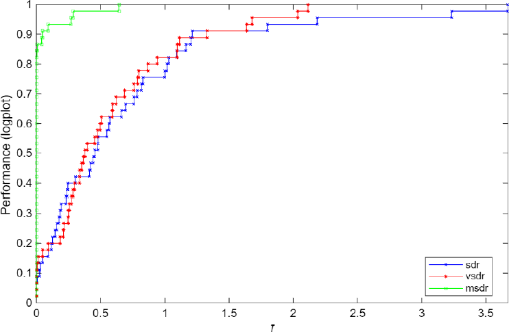
To compare computational efficiency, we analyze CPU time using the Dolan-Moré performance profile (Dolan & Moré, 2002). As shown in Fig. 3, MSDR appears as the dominant method within this group, indicating superior performance in terms of CPU time.

In addition to the group-based comparison, we construct a global performance profile that includes all instances and all methods. For each problem and method, the performance ratio is defined relative to the best-performing method in terms of CPU time, provided that the method attains the best objective value (within a tolerance of 10⁻⁶). Otherwise, including cases where a method produces an inferior objective value or fails to converge within the time limit, it is treated as unsuccessful and assigned an infinite performance ratio.

Following the Dolan-Moré framework (Dolan & Moré, 2002), such unsuccessful cases result in curves that may not reach one, thereby reflecting both computational efficiency and robustness.

Figure 4
Performance profile considering all instances and all methods.

The resulting performance profile is shown in Fig. 4. It can be observed that MSDR dominates the other methods over a large range of performance ratios, indicating superior computational efficiency. In contrast, SSDR performs best on a subset of instances, achieving higher probabilities in certain regions, which reflects its competitiveness in terms of robustness. In addition, the methods SSDR+RRLT, ESDR, and AESDR are consistently reported as failures, confirming their lack of practical competitiveness in this study.

10.3 Comparison of Semidefinite Relaxations for BQP-GUB

Table 4 provides an overall comparison of semidefinite relaxations for BQP-GUB.

Table 4
Comparison of semidefinite relaxations for BQP-GUB.

Relaxation Method	Tightness	Scalability	Overall Effectiveness	Best Use Case
SDR (classical)	Loose	High	Weak relaxation	Baseline comparison
SSDR	Not tight	High	Moderate	Large-scale problems
SDR+RRLT	Very tight	Moderate	Strong	Small-medium problems (n ≤ 100)
SSDR+RRLT	Very tight	Low	Strong but limited	Small problems (n ≤ 50)
ESDR	Improved SDR	Low	Least effective	Rarely recommended
AESDR	Improved SDR	Low	Least effective	Rarely recommended
VSDR	Same as SDR	High	Moderate	Large-scale problems needing speed
MSDR	Same as SDR	High	Moderate	Large-scale problems needing speed

11 CONCLUSION

In this paper, we studied semidefinite programming (SDP) relaxations for the BQP-GUB problem through a unified theoretical and computational framework. We showed that several formulations, including SDR, VSDR, and MSDR, as well as SSDR and ESDR, are equivalent in terms of bound quality. Our results indicate that improvements in relaxation strength arise primarily from the incorporation of stronger valid constraints, particularly reduced reformulation linearization techniques (RRLT), rather than from alternative SDP formulations. RRLT-based relaxations, such as SDR+RRLT and SSDR+RRLT, yield tight or near-tight bounds and significantly reduce the relaxation gap. However, this comes at the expense of increased computational cost, limiting their scalability for large-scale instances, whereas simpler relaxations remain computationally efficient.

Overall, the study clarifies the relationships among SDP formulations for BQP-GUB and high-lights the trade-off between bound quality and computational scalability. Future work will focus on developing scalable strengthened relaxations and exploiting problem structure to improve efficiency.

Acknowledgements

This research work is fully supported by the National Board for Higher Mathematics (NBHM), Department of Atomic Energy, Govt. of India (Grant no. 02011/22/2021 NBHM (R.P.)/R&D II/900 Date 06/08/2021).

Data Availability

The datasets analyzed during the current study are available on the web address: BQP-GUB (https://sites.google.com/a/iiit-bh.ac.in/r-k-nayak/bqp-bqp-problems/bqp-gub-problems).

References

• ANSTREICHER K, CHEN X, WOLKOWICZ H & YUAN YX. 1999. Strong duality for a trust-region type relaxation of the quadratic assignment problem. Linear Algebra and its Applications, 301(1-3): 121-136.
• ANSTREICHER K & WOLKOWICZ H. 2000. On Lagrangian relaxation of quadratic matrix constraints. SIAM Journal on Matrix Analysis and Applications, 22(1): 41-55.
• ANSTREICHER KM. 2009. Semidefinite programming versus the reformulation-linearization technique for nonconvex quadratically constrained quadratic programming. Journal of Global Optimization, 43: 471-484.
• BECK A. 2007. Quadratic matrix programming. SIAM Journal on Optimization, 17(4): 1224-1238.
• BECK A & TEBOULLE M. 2000. Global optimality conditions for quadratic optimization problems with binary constraints. SIAM Journal on Optimization , 11(1): 179-188.
• BOYD S & VANDENBERGHE L. 2004. Convex optimization. Cambridge university press.
• BYRD RH, NOCEDAL J & WALTZ RA. 2006. Knitro: An integrated package for nonlinear optimization. Large-scale nonlinear optimization, pp. 35-59.
• CHHAJED D & LOWE TJ. 1992. m-median and m-center problems with mutual communication: Solvable special cases. Operations Research, 40(1-supplement-1): S56-S66.
• CHRÉTIENNE P. 1989. A polynomial algorithm to optimally schedule tasks on a virtual distributed system under tree-like precedence constraints. European Journal of Operational Research, 43(2): 225-230.
• DEMAINE ED, EMANUEL D, FIAT A & IMMORLICA N. 2006. Correlation clustering in general weighted graphs. Theoretical Computer Science, 361(2-3): 172-187.
• DING Y & WOLKOWICZ H. 2009. A low-dimensional semidefinite relaxation for the quadratic assignment problem. Mathematics of Operations Research , 34(4): 1008-1022.
• DOLAN ED & MORÉ JJ. 2002. Benchmarking optimization software with performance profiles. Mathematical programming, 91(2): 201-213.
• FAYE A & ROUPIN F. 2007. Partial Lagrangian relaxation for general quadratic programming. 4OR, 5: 75-88.
• FINSLER P. 1937. Uber das vorkommen definiter und semidefiniter formen in scharen quadraticher formen. Commentarii Mathematici Helvetici, 1: 19-28.
• FONTAN F, FERREIRA A, BUSCAYLET F & ALIOUAT I. 2022. Résolution de problèmes MINLP avec Artelys Knitro 13.0. In: 23ème congrès annuel de la Société Française de Recherche Opérationnelle et d’Aide à la Décision.
• GELENBE E, TIMOTHEOU S & NICHOLSON D. 2010. Fast distributed near-optimum assignment of assets to tasks. The Computer Journal, 53(9): 1360-1369.
• GRANT M, BOYD S & YE Y. 2009. CVX: Matlab software for disciplined convex programming.
• GREENBERG H. 1969. A quadratic assignment problem without column constraints. Naval Research Logistics Quarterly, 16(3): 417-421.
• GUATTERY S & MILLER GL. 1998. On the quality of spectral separators. SIAM Journal on Matrix Analysis and Applications , 19(3): 701-719.
• HEILER M, KEUCHEL J & SCHNÖRR C. 2005. Semidefinite clustering for image segmentation with a-priori knowledge. In: Joint Pattern Recognition Symposium. pp. 309-317. Springer.
• JOULIN A, BACH F & PONCE J. 2010. Discriminative clustering for image co-segmentation. In: 2010 IEEE Computer Society Conference on Computer Vision and Pattern Recognition. pp. 1943-1950. IEEE.
• KANNAN R, VEMPALA S & VETTA A. 2004. On clusterings: Good, bad and spectral. Journal of the ACM (JACM), 51(3): 497-515.
• KLEINBERG J & TARDOS E. 2002. Approximation algorithms for classification problems with pairwise relationships: Metric labeling and Markov random fields. Journal of the ACM (JACM) , 49(5): 616-639.
• LANG K. 2005. Fixing two weaknesses of the spectral method. Advances in Neural Information Processing Systems, 18.
• MOSEK A. 2017. The MOSEK optimization toolbox for MATLAB manual, version 8.0 (Revision 60).
• NAYAK RK & MOHANTY NK. 2019. Improved row-by-row method for binary quadratic optimization problems. Annals of Operations Research , 275(2): 587-605.
• SCHELLEWALD C & SCHNÖRR C. 2005. Probabilistic subgraph matching based on convex relaxation. In: International Workshop on Energy Minimization Methods in Computer Vision and Pattern Recognition. pp. 171-186. Springer.
• SHERALI HD & ADAMS WP. 2013. A reformulation-linearization technique for solving discrete and continuous nonconvex problems. vol. 31. Springer Science & Business Media.
• SHERALI HD, DALKIRAN E & LIBERTI L. 2012. Reduced RLT representations for nonconvex polynomial programming problems. Journal of Global Optimization , 52: 447-469.
• VITALADEVUNI SN & BASRI R. 2010. Co-clustering of image segments using convex optimization applied to EM neuronal reconstruction. In: 2010 IEEE Computer Society Conference on Computer Vision and Pattern Recognition. pp. 2203-2210. IEEE.
• WANG Y & PUNNEN AP. 2017. The boolean quadratic programming problem with generalized upper bound constraints. Computers & Operations Research , 77: 1-10.
• ZHAO Q, KARISCH SE, RENDL F & WOLKOWICZ H. 1998. Semidefinite programming relaxations for the quadratic assignment problem. Journal of Combinatorial Optimization, 2: 71-109.

Edited by

• Editor responsible for the review
  Editor-in-Chief: Antônio Augusto Chaves

Publication Dates

• Publication in this collection
  31 July 2026
• Date of issue
  2026

History

• Received
  16 Sept 2025
• Accepted
  21 May 2026