Hydrodynamic modelling in the Amazonian Estuary: A flexible mesh approach

ABSTRACT

Several hydrodynamic models have been applied to the Amazonian Estuary, but its complex shape makes the grid definition difficult when a structured grid is used. This research aims to implement a hydrodynamic model for this estuary based on a flexible mesh grid system and then analyze the results. The methodology is based on Delft3D FM, and the model domain encompasses the low course of the Amazon, Tapajos, Xingu, Tocantins, and Para rivers, Guajara and Marajo bays, and Breves Strait, as well as the floodplain areas and the adjacent continental shelf. The model simulation performs well against the observed tidal water levels and instantaneous transport since Pearson’s correlation coefficient showed more significant values than 95% for both, and root mean square error (RMSE) showed smaller values than 5% for water levels and 15% for instantaneous transport. This also performs well in simulating scenarios representing different tide and instantaneous transport conditions.

Keywords:
Delft3D FM; Manning’s coefficient; tropical estuary; Amazon River

INTRODUCTION

Estuaries have biological, economic, and social importance. Their dynamics and morphology enable them to shelter several biological species and the development of economic activities, such as ports, fishing, tourism, and aquaculture. These characteristics have made estuaries attractive for human life, thus, they are usually widely populated. The Amazonian Estuary comprises several water bodies, including the Amazon River, Tapajos River, Xingu River, and Tocantins River, which are in the sixth group of the world’s largest 20 rivers (Dai and Trenberth, 2002). This estuary flows into the continental shelf with a seven runoff of about 7.28 x 10¹² m³/year (average 230.000 m³/s) (Mikhailov, 2010).

There are many water bodies in the Amazonian Estuary as well as a large area of flood plains; for instance, Mertes et al. (1996) mentioned that the Amazon River floodplain constitutes of lakes, lake deposits, floodplain channels, scroll bars, and over bank deposits. Several modelling techniques have been applied to the Amazonian River/Estuary system. Some examples are Nikiema et al. (2007) and Vinzon and Paiva (2002), who use these techniques mainly to analyze the continental shelf dynamics, including water runoff and sediment transport. Gabioux et al. (2005) made tidal propagation analyses by applying modelling on a large scale. Nevertheless, the curvilinear mesh grids widely used in these models are not easily defined because of many water bodies and floodplains in the study area.

Works such as Fontes et al. (2008), Bars et al. (2010), and Nikiema et al. (2007) have modeled some aspects of these two systems’ estuary. They mainly used unstructured curvilinear and orthogonal grids and obtained good results regarding hydrodynamics, Amazon plume, tidal conditions, and bottom stress. However, the full integration of the fluvial part of these systems with their tributaries, considering both fluvial and marine forces, is still a challenge. To conduct an approach that mainly helps to define the large number of tributaries in this region, this work used a flexible mesh via the Delft3D Flexible Mesh, which has one of its main advantages, the combination of unstructured curvilinear meshes with triangles, pentagons, and 1D channel networks, thus providing greater flexibility to the mesh. Another advantage is its efficiency in solving matrices, which combines the conjugate gradient method and the minimum degree method (Deltares, 2014; Kernkamp et al., 2011).

Such advantage saves computational effort, so several smaller tributaries were included in the systems as 1D channels to reduce computational effort. The model simulation has already been applied to systems such as the Guayas River Estuary (Ecuador), the San Francisco Bay-Delta (USA), and the Columbia River Estuary (USA), representing the various physical aspects of concern within each system with great accuracy (Achete et al., 2015; Crespo, 2016; Putra et al., 2015). Therefore, this research aims to implement a hydrodynamic 2D barotropic model of the Amazonian Estuary based on a flexible mesh grid that is easier to define than curvilinear grids on this kind of system to analyze the hydrodynamic patterns within this estuary.

METHODS

PHYSICAL AREA DESCRIPTION

The Amazon River is a tidal river that flows until the section near the city of Obidos, which is characterized as an upper tidal river (Fricke et al., 2018). This is branched and has a funnel shape in the downstream area, characteristics that are associated with estuaries (Sioli, 1984). The funnel shape also enables the classification of the Amazon River basin mouth as a coastal plain dominated by tides, in which the tidal currents are the main factor for morphological changes. A semidiurnal meso and macrotide drive the estuarine area that penetrates the estuary around 1,000 km from the coastline (Beardsley et al., 1995; FEMAR, 2000).

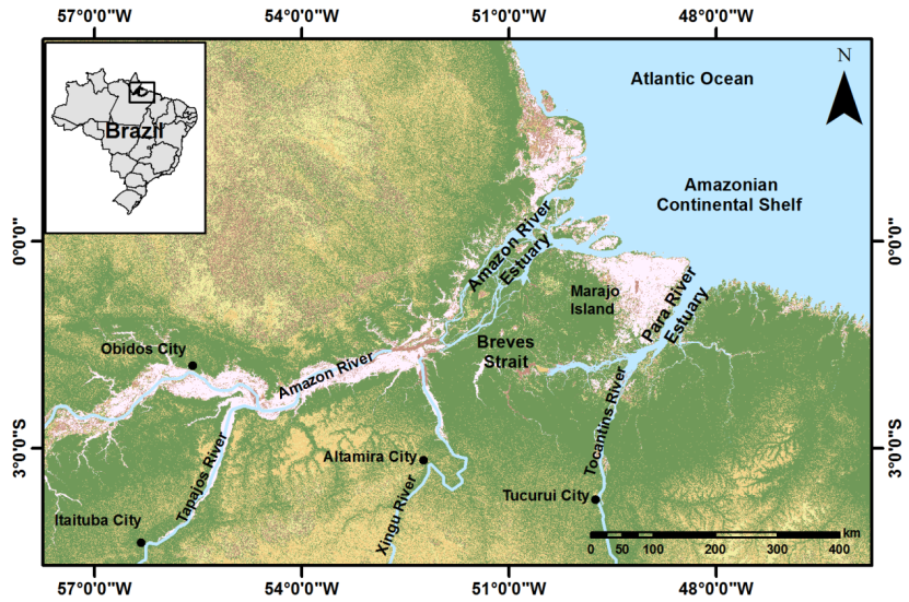
The Amazonian Estuary has two main branches. The first is the Amazon River Estuary, which flows on the west side of Marajo Island and carries most of the Amazon River’s water into the Atlantic Ocean, with most of the Amazon River water runoff. The second, Para River Estuary (PRE), is connected with the former by a system of channels called Breves Strait, which flows on the east side of Marajo Island and is powered by the Tocantins water system and Guajara Bay (Figure 1).

Figure 1
Location of the Amazonian Estuary and its major water bodies.

Regarding the circulation patterns, there are different classifications for the Amazon River Estuary and the PRE. Some authors classify these two systems as a well-mixed estuary (Baltazar et al., 2011; Menezes et al., 2011). Such authors usually consider measurement points inside the estuary until its mouth with salinity values is less than 10. Nevertheless, some investigations on the adjacent continental shelf show this estuary is a stratified system in which an estuarine plume is dispersed to the continental shelf due to the high river system discharge (Geyer et al., 1996), in which salinity values between 15 and 35 can be found.

Salinity gradients are mainly driven by river discharge and tidal currents. The drainage of the Amazon River basin is very complex and is formed by more than 500 larger rivers and uncountable other small water bodies (Dai and Trenberth, 2002). Still, this research focused on the downstream area, in which the main tributaries are the Tapajos River, Xingu River, and Tocantins River. Table 1 describes these rivers. The rivers that flow into the Amazon Estuary are mainly fed by runoff from the drainage basin, which is fed by rain. In addition, the Amazon river has the highest discharge months between April and July, whereas for the Tocantins River, one of the main tributaries of the PRE, it occurs between February and May (Costa et al., 2003; Geyer et al., 1996; Masson and Delecluse, 2001; Dai and Trenberth, 2002; Prestes et al. 2020). The climate of the study area is equatorial, hot, and humid, encompassing the climatic types Am and Af, according to the classification of Köppen (1936) (Alvares et al., 2013). The mean annual temperature, air humidity, and annual rainfall are 25 ºC, 80%, and 2,889 mm/year, respectively. In the Amazon Basin area, the maximum rate of atmospheric precipitation occurs between February and August. Still, the maximum rate of atmospheric precipitation in the estuarine area occurs between February and May. Consequently, the largest river discharge occurs between May and July since it is expected to have some delay in response to the atmospheric precipitation rate (Sioli, 1984; Dai and Trenberth, 2002; Mikhailov, 2010).

Table 1
Characteristics of the main rivers (Source: Dai and Trenberth, 2002; Mikhailov, 2010).

River	Total drainage area km2	Average annual discharge m3/sec	Annual discharge km3/year	Sediment Runoff t/year
Amazon (Obidos)	4.68x106	1.73x105	5460	1.26 x 109
Tapajos	5.02 x105	-*	415	-*
Xingu	4.97 x105	1.60 x104	302	3.43 x 106
Tocantins	7.69 x105	1.63x104	511	3.06 x 106

• *no data

The estuary bathymetry is irregular, with longitudinal sand bars and channels constructed by the tidal currents and river flow. The depths are around 20 m inside the estuary and reach 100 m on the continental shelf (but these values can be much bigger for both in some areas). Although the estuary is driven by tide, the waves play an important role by resuspending sediments and forming estuarine beaches. Thus, the sediment distribution results from the combination of tidal currents, river currents, and wave action, with the latter affecting the riverbanks on a small scale (Gregório and Mendes, 2009).

The bottom sedimentology consists mainly of medium sand to clay. The coarse sediment grain size can be found in the internal part of the estuary; on the mouth portion in contact with the Atlantic Ocean, the sediment can be found at a finer grain size (Costa et al., 2003; Corrêa, 2005; Costa et al., 2013). Corrêa (2005) also describes a transversal variation of the sediment grain size due to ebb and flood currents during a tidal cycle.

The Amazon Estuary and the adjacent Amazon Continental Shelf are governed by a complex system of overlapping forces, mainly tides, wind, and river discharge. This region has tidal heights that vary from two to 11 m, in which M2 is the component with the most significant amplitude, reaching values of up to 3 m (Beardsley et al. 1995; Bars et al. 2010). Salinity ranges from zero to 35, depending on the proximity to the Amazon and Para River estuaries and climatic seasonality (Fontes et al., 2008; Geyer et al., 1996; Kineke et al., 1996).

This mouth region shows significant turbulence and intense advective and mixing processes, mainly because of the depth (reduced in the mouth of the system, with depth < 10 m) combined with the effects of tides, water discharge, and wind action. As one travels from the mouth of the Amazon River towards the nearby ocean, the vertical structure of the water column changes from barotropic to baroclinic, in which oceanic water is concentrated at depth, and plume water extends over the entire sea surface (Fontes et al., 2008).

MODEL

DOMAIN AND GRID

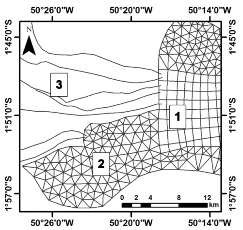
Delft3D Flexible Mesh was used to simulate the hydrodynamics of the Amazon Estuary. This is a 1D-2D- 3D hydrodynamic simulation package in development (until the conclusion of this research) by Deltares in cooperation with the Delft University of Technology, in the Netherlands. This was based on numerical concepts of Delft3D and SOBEK1D2D, but the advantage of Delft3D Flexible Mesh is the possibility to define flexible mesh grids (Figure 2) that are curvilinear meshes combined with other grid elements, for instance, triangles and pentagons as well as 1D-channel networks (Kernkamp et al., 2011).

Figure 2
Flexible mesh grid: a combination of curvilinear mesh (1) with triangles (2) and 1D channel networks (3).

Because of the highly dynamic study area, with mixing processes that prevent stratification along the water column, it was decided to apply 2D and 1D meshes to the domain. This approach, which was already used by Rosario (2016), is sufficient to reproduce the phenomena that occur in the Amazonian estuary system.

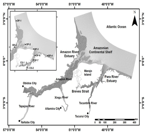
The domain encompasses the main rivers and channels of the Amazonian Estuary System (Amazon River, Tapajos River, Xingu River, Tocantins River, Guajara Bay, Marajo Bay, Breves Strait, and Para River), the floodplain area, and the continental shelf adjacent (Figure 3). The domain covers approximately 700 km along the coastline and 145 km offshore. This domain reaches 716 km upstream through the Amazon River and 430 km through the Para River/Tocantins River. This study considers floodplain due to its low topography, macro-tidal regimes, and seasonal variation in river discharge. This dynamic enables large areas to be flooded, and fluid exchanges between the main channel and the tidal plain occur throughout the entire domain.

Figure 3
Domain and flexible mesh defined grid and location of observation points (OP), and cross-section (CS) used during validation.

The model’s boundary occurs at an altitude of 10 m throughout the domain, except for the area where the 1d channels were applied, assuming areas of wetting/drying. The elements resolution would be by the local altimetric variation, i.e., the greater the local altimetric variation, the smaller the element’s size. Curvilinear meshes combined with triangles and 1D-channel networks were used during the mesh definition (Figure 3). The curvilinear meshes were applied to the main rivers (Amazon River, Tapajos River, Xingu River, and Tocantins Rivers) and continental shelf. Triangular cells were applied to floodplains and to link curvilinear meshes with different numbers and sizes of cells, with resolution varying from 0.005 km to 4 km. 1D-channel networks were defined for relatively small Breves Strait channels with widths being smaller than 5 km and variable depth, with a rectangular cross-section.

The 1D channels have the highest mesh resolution (0.005 km), enabling an increase in the number of elements in these channels without sacrificing computational effort and performance. The orthogonalization parameter regarding mesh smoothness and orthogonally showed values that are smaller than 0.06. The parameter for orthogonalization should have the smallest possible value (>0) and should not exceed 0.1. Such values were relatively easy to achieve due to a flexible mesh. This orthogonality parameter value was applied to all the grid elements, whether triangular or quadrilateral.

The equations system used in Delft 3D can be found in the user manual of Delft 3D FLOW, a simulation of multi-dimensional hydrodynamic flows and transport phenomena, including sediments (Deltares, 2023). This is based on the works of Kernkamp et al. (2011), Crespo (2016), and Achete et al. (2015). The equations consist of the horizontal equations of motion, the continuity equation, and the transport equations for conservative constituents, solving the unsteady shallow water equations in two (depth-averaged) or three dimensions.

The model package includes mathematical formulations that consider several physical phenomena, such as baroclinic and barotropic effects, equation of state, Coriolis force, turbulence closure models, transport of conservative constituents such as salt and heat, tidal forcing (at the open boundaries) and tidal generating forces, wind shear-stress at the water surface and time-varying sources and sinks, like river discharge (Deltares, 2023).

BATHYMETRY

The bathymetry interpolation was based on different data sets: 116 charts from the Brazilian Department of Hydrography and Navigation (DHN) of the continental shelf, estuaries, and rivers of the study area (mainly the 221 and 232 nautical charts), and bathymetry from GEBCO 08 (General Bathymetric Chart of the Oceans) a continuous terrain model for ocean and land with a spatial resolution of 30 arc-seconds, via Delft Dashboard, an open-source MatLab-based user interface that was developed by Deltares (van Ormondt et al., 2020). The second one was used to fill in missing values that were not found in nautical charts (mainly in floodplain areas).

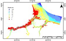
During the validation process, we manually adjusted bathymetry due to the grid cell size to ensure reliable interpolation. For instance, sample points for features such as sandbars, small islands, or deep channels may fall within the same cell. As a result, the interpolation led to either shallow channels or channels that were abruptly obstructed, producing inaccurate numerical water levels and numerical instantaneous transport values in subsequent hydrodynamics. Manual adjustments were made in the bathymetry cells corresponding to river channels and the continental shelf, and a constant and smooth slope was defined (Figure 4) using the sample values as a guideline. Such adjustments avoided abrupt changes in the bathymetry and resulted in well-defined channels.

Figure 4
Bathymetry after manual adjustment.

ROUGHNESS

The roughness coefficient means flow resistance in a channel or a flood plain. The Manning’s coefficient was used during this research. The roughness coefficient values were given to the domain based on Arcement Jr. and Schneider (1989), citing the Cowan (1956) procedure. This procedure determines the effects of channel characteristics on Manning’s roughness coefficient (hereafter to be called n) value. The following formula can determine the value of n:

$n=\left(n_b+n_1+n_2+n_3+n_4\right)m·$ /1/

In which: n_b is a base value of n based on the surface sediment of the channel or flood plain; n₁ is a correction factor regarding the effect of surface irregularities (or surface roughness); n₂ is a correction factor regarding the variations in the shape and size of the channel or floodplain; n₃ is a correction factor regarding the obstruction to the flow; n₄ is a correction factor regarding the presence and density of vegetation, and; m is correction factor for meandering of the channel (not applicable to floodplains for which m=1).

The area regarding the continental shelf close to the Amazon River and Para River mouths received a very small roughness coefficient, n=0.015; however, the smallest roughness coefficient of n=0.013 was defined to the Amazon Estuary between the continental shelf and the Xingu River mouth. Such values were founded on the fact that the bottom is mainly composed of mud, and the area has a high degree of suspended sediment and the occurrence of fluid mud Discharge and sea boundaries.

The river discharge input was defined based on a data set on the National Water Agency (ANA, 2015) website. Using 30 years of data, the mean monthly discharge for each river was estimated (Figure 5). The discharge data for the Amazon River was taken in Obidos City, the Tapajos River in Itaituba City, the Xingu River in Altamira City, and the Tocantins River in Tucurui City (Figure 3). These cities were chosen to avoid problems with tidal waves on upstream open boundaries, as tidal waves reach long distances inside the river system, such as resonance between harmonics.

Figure 5
The 30-year mean of monthly discharge data between 1980 and 2010 to the source upstream of the main rivers in the Amazon region.

The sea level boundary condition was defined based on Regional Tidal Solutions (OTIS - available at http://g.hyyb.org/archive/Tide/TPXO/TPXO_WEB/global.html) data for Amazon Shelf, and the components used were M2, S2, N2, K1, O1, and M4. The regional inverse solution fits the data significantly better for complex topographic areas and in shallow water - which occurs on the continental shelf adjacent to the Amazonian Estuary System- when compared with TPXO global solutions (Egbert and Erofeeva, 2002).

Thus, OTIS data were used for the offshore boundary conditions of the model, and the flow was used for the river heads. Changes in salinity, temperature, and suspended sediment were ignored. Furthermore, since the model package does not respond to oceanic and outer shelf processes, the focus was only on the continental and inner shelves.

The instantaneous transport was estimated from the data collected in situ, in the Para and Tocantins River, with an Acoustic Doppler Current Profiler (ADCP), model Workhorse Monitor (600 kHz) Teledyne, RD Instrument. The data acquisition was performed by hourly sampling along the cross-section of the estuarine channel during a tidal cycle (13 h) in July during the wet season (Figure 3, CS-1, and CS-2). The collected velocity and direction data were analyzed and processed as Miranda et al. (2017) described and used to calculate the instantaneous transport in m³/s. The data were used for model validation.

Note that the discharge used in the model simulation input is characterized as the river component of the system, excluding the bidirectional tidal oscillation, and the instantaneous transport (m³/s) is obtained by each instant in time. The resultant instantaneous transport is defined as the temporal average resulting from the instantaneous transport over a tidal cycle, which is the product of the u-component of the velocity (m/s) and the cross-sectional area (m²) integrated over the entire cross-sectional area (Miranda et al. 2017, Miranda et al. 1998, Moser et al. 2005).

According to Abreu et al. (2020), the discharge term does not represent a resultant but rather the oscillation of instantaneous transport during a tidal cycle. Studies, such as Thomson and Emery (2014), Miranda et al. (2017), and Moser et al. (2005), use the term instantaneous transport to refer to the transport of flood (negative) and ebb tide (positive) during a tidal cycle. Moser et al. (2005) still use the same term to refer to a resultant over a tidal cycle, characterized as net discharge by Simpson and Bland (2000).

The main difference between discharge (Figure 5) and instantaneous transport for this study is the tidal influence and the time series used for each analysis. This paper uses the term discharge to characterize the river component used as model input. Numerical instantaneous transport is the model output analyzed for a tidal cycle. Real instantaneous transport was estimated from data collected in situ, considering both negative and positive transport values.

In addition, to validate the model simulation, seven observation points (OP) and two cross-sections (CS) were used (Figure 3). The stations are distributed on the estuary mouth and coastline. Harmonic analysis data for each station are available on the FEMAR (Fundação de Estudos do Mar) website. The cross-sections are located on Breves Strait and Tocantins River mouth to calibrate the flow within the estuary. For these CS, a data survey was conducted during one tidal cycle (13 h) in July (wet season). Main metrics that were considered during the validation process: Pearson’s correlation coefficient and root mean square error (RMSE). Tidal components analysis was also considered during the validation of OP and instantaneous transport for CS.

Pearson’s correlation coefficient determines a linear relationship for two variables, but the same correlation value can represent a set of correlation scenarios; due to this, the RMSE was applied to determine the error (dimensional), thus giving a better interpretation of results. The resultant instantaneous transport was defined from two sectors at the estuary mouth. The first is on the west side of Marajo Bay for L1, L2, L3, and L4, and the second is on the east side of Marajo Bay for L5, see Figure 8 for the locations of transects.

WIND

Curtin and Legeckis (1986) determined wind from the east with a magnitude between 3-12 m/s and a direction between 60-100 degrees true north based on some sampling analyses on the Amazon continental shelf. The wind magnitude and direction values defined for the Amazon Estuary modelling were 8 m/s and 80 degrees true north. The wind was considered constant in time and space to make the model simulation more controllable during validation. Wind data were added to the model simulation as fine-tuning since it did not significantly change the hydrodynamics.

TIME SETUP

The model simulation was set with a maximum time step of five minutes, and the Courant parameter used was 0.7. This value is the highest that the model accepts, and values higher than 0.7 generate errors due to the variability of the elements. The model simulation was running into three different setups, each with a simulation time equal to one month (July 2013) for the simulation to reach a physical equilibrium and one month to simulate the different scenarios. The first setup was used for validation, the second one to simulate the dry period, and the third one to simulate the wet period. During the validation, the considered month was July (available in situ instantaneous transport data for validation); for dry season simulation and wet season, the considered months were November and May, respectively.

RESULTS

NUMERICAL RESULTS VALIDATION

Figure 6 shows time series plots for each OP to compare the amplitude and the calculated and real signals phase (tidal prediction based on harmonic analysis). Table 2 contains the amplitude of the main tidal components, and Table 3 contains the statistical results. The model simulation result was underestimated on observation point one (OP1) even though the calculated values are in phase with validation values. The difference in amplitude can be attributed mainly to M2 and M4. The RMSE was 0.50 m, which was considered acceptable since the tidal range shows variation between 6 m and 9 m for the considered period.

Figure 6
Time series comparison plot for water level for June 2014.

Table 2
Simulated (sim) and real amplitude (in meters) of major tidal components.

Obs. Point	O1		NO1		K1		N2		M2		S2		MN4		M4		MS4
	real	sim	real	sim	real	sim	real	sim	real	sim	real	sim	real	sim	real	sim	real	sim
1	0.14	0.15	0.02	0.05	0.16	0.21	0.49	0.36	2.69	2.23	0.47	0.35	0.00	0.10	0.04	0.29	0.00	0.10
2	0.07	0.12	0.01	0.04	0.11	0.16	0.31	0.31	1.87	1.78	0.36	0.34	0.00	0.09	0.29	0.29	0.00	0.09
3	0.13	0.08	0.01	0.03	0.14	0.11	0.23	0.26	1.15	1.45	0.28	0.31	0.00	0.04	0.32	0.14	0.00	0.05
4	0.12	0.11	0.02	0.02	0.15	0.15	0.34	0.41	1.86	2.07	0.36	0.51	0.00	0.00	0.11	0.06	0.00	0.00
5	0.06	0.09	0.01	0.02	0.13	0.11	0.17	0.13	1.01	0.81	0.17	0.14	0.00	0.05	0.22	0.16	0.00	0.05
6	0.10	0.06	0.01	0.02	0.12	0.08	0.23	0.22	1.38	1.30	0.29	0.26	0.00	0.06	0.09	0.16	0.00	0.07
7	0.11	0.05	0.01	0.01	0.13	0.06	0.20	0.18	1.11	1.10	0.23	0.21	0.00	0.05	0.01	0.14	0.00	0.05

Table 3
Pearson’s correlation coefficient, root mean square error for water level in which the real and calculated values are compared, in addition to approximated tidal range.

Station	Pearson correlation coefficient	Root mean square error (m)	Max. tidal range (m)
Station 1	0.9802	0.5157	7.91
Station 2	0.9872	0.2283	5.42
Station 3	0.9664	0.3270	4.03
Station 4	0.9861	0.3061	6.04
Station 5	0.9750	0.2162	3.90
Station 6	0.9804	0.2072	4.01
Station 7	0.9765	0.1835	3.49

Observation points two, three, and four (OP2, OP3 and OP4) are also located at the coastline, but the results were overestimated, mainly during the spring tide. The difference in amplitude can be attributed mainly to MN4 and MS4 for OP2, and M2 for OP3 and 4. The RMSE was acceptable, around 0.30 m, because the tidal range shows values around 5 m.

The results for OP1, located northwest of Amazon River, show the biggest RMSE considering the tidal range on this location (almost 8 m during the spring tide for the analyzed period). This error can be mainly attributed to the irregular bathymetry and the tidal components M2, MN4, M4, and MS4, which showed significant differences values (Table 2). In addition, the extreme conditions of turbulence and high kinect energy for the northwest of the Amazon River mouth (Carneiro and Rollnic, 2024), could also contribute to the large difference between the real (or observed) and simulated (or calculated) in OP1.

Observation points six and seven (OP6 and OP7) on Para River show good validation. These RMSE have values of 20 cm, representing 5% of the local tidal range. In OP1, OP3, and OP5, the tidal components M2, MN4, M4, and MS4 reach the most significant difference when calculated and real values are compared. Nevertheless, M4 was the main tidal component that created the error for OP1 and OP3, with an approximate difference of 20 cm between simulated and real values. The model shows a reasonable performance since in simulating tidal signal ,as the Pearson’s correlation coefficients are around 0.98 and the RMSE values are not bigger than 10% of the mean local tidal range (Table 3).

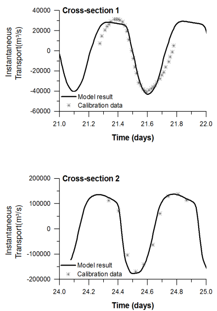
Figure 7 and Table 4 show real and numerical instantaneous transport. Figure 7 shows time series plots for each CS to compare the amplitude and phase of calculated and real signals. Table 5 contains the statistical results and the instantaneous transport for real and numerical mean values for one tidal cycle (resultant instantaneous transport).

Figure 7
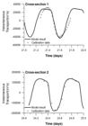
Time series comparison plot for instantaneous transport. Positive values indicate instantaneous transport towards the mouth, and negative values towards the upstream.

Table 4
Pearson’s correlation coefficient, root mean square, and instantaneous transport resultant of CS-1 and CS-2.

Cross-section	Pearson correlation coefficient	Root mean square error (m³/s)	Instantaneous transport (m3/s)		Considered Period (hours)
			real	simulated
1	0.9624	1.5 x 104	-4.13 x 104	-1.65 x 104	12
2	0.9840	1.7 x 104	4.75 x 105	5.41 x 105	12.96

Table 5
Numerical resultant instantaneous transport values for the eight simulated scenarios in 10⁴ m³/s per tidal cycle.

Scenario	L1	L2	L3	L4	L5
Jun/neap	986	-5	2	930	194
Jun/spring	872	-14	-6	808	19
Oct/neap	475	-3	-9	536	104
Oct/spring	493	-10	-12	494	78
Nov/neap	457	-5	-10	489	78
Nov/spring	397	-10	-14	423	78
Apr/neap	931	-6	-2	921	293
Apr/spring	975	-12	-3	904	218

Analysis of cross-sections instantaneous transport shows promising results of Pearson’s correlation and RMSE. The correlation is more significant than 95% and the RMSE is smaller than 15%, showing the numerical and real match in direction and magnitude. In addition, the numerical instantaneous transport also shows a difference of 61% higher than the real value for CS-1. In CD-2, the difference between simulated and real values of instantaneous transport was about 15%.

Note that the negative values being higher than the positive values are probably due to the seasonality period used in the model validation. The acquisition date was during the transition period in the region, characterized by decreasing discharge of the Amazon River, which has the lowest discharge between October and December (Curtin and Legeckis, 1986; Geyer et al., 1996). Therefore, even with the contribution of 1% of the Amazon River discharge to the Para River through the Breves Strait (Callède et al., 2010; Prestes et al., 2020), the absolute flow values vary due to the region’s seasonality. Thus, it is possible to have a resultant instantaneous transport upstream in CS-1, considering, for example, a semi-diurnal tidal cycle and spring tidal conditions.

The choice of a single tidal cycle for calibration and comparison was due to the hydrodynamics of the region, mainly controlled by the freshwater discharge from the Amazon River and tidal oscillation. Therefore, the selected tidal cycle had the most significant variation in tidal height (in meters) throughout the month. Any other tidal cycle in the same period tends to have resultant instantaneous transport values equal to or lower than the simulated one.

HYDRODYNAMIC ANALYSES

Five cross-sections were defined (Figure 8 - L1 to L5) within the estuary mouth to create information about discharge in different scenarios to analyze some hydrodynamic patterns of the Amazon Estuary. The scenarios are (1) spring tide/wet season, (2) neap tide/wet season, (3) spring tide/dry season, and (4) neap tide/dry season.

Figure 8
Location of the five cross-sections (L1 to L5) to quantify the mean for instantaneous transport (order to 10⁴ m³/s) and the resulting vector after one tidal cycle for eight scenarios.

The external channels of the Amazonian River Estuary (L1 and L4) show higher values of mean instantaneous transport when compared to its internal channels (L2 and L3). External channels show values of 698.25 and 688.12 x 10⁴ m³/s for L1 and L4, respectively. The results provide high values of resultant instantaneous transport for both branches of the Amazonian Estuarine System. Another difference between the external and internal channels is the direction of resultant instantaneous transport (Table 5): L1 and L4 show runoff in the downstream direction (positive values), and L2 (-8.12 x 10⁴ m³/s) an L3 (-6.75 x 10⁴ m³/s) in the upstream direction (negative values). The PRE (L5) shows a magnitude of instantaneous transport of 132.75 x 10⁴ m³/s.

DISCUSSION

Some OPs for the water level validation showed overestimated results (OP 2, 3, and 4 - Table 2), mainly during spring tide. This variation can occur due to the difference in bathymetry and morphology between the real and simulated scenarios, which may lead to overestimation or underestimation of the model, since these areas have many channels and small estuaries that are not in the model simulation (Deltares, 2014; Deltares 2023). The absence of these small features amplifies the tidal range, mainly during spring tide.

Moreover, the major tidal components showed differences between numerical and real results. The main differences in tidal signals are regarding the tidal components M2 as well as MN4, M4, and MS4, which reinforces the hypothesis that bathymetric differences are the main cause of that, considering that the quarter-diurnal tidal components are influenced by the interaction of the wave with the bottom (Parker, 1991). Nevertheless, wind seasonality and river discharge can induce variations in the response of the tidal components (Voinov, 2007), considering that a constant wind in time and space and mean monthly discharges were applied during the modelling.

The results for the instantaneous transport showed a significant difference between the real x simulated results in CS-1. This indicates a necessity to define the mesh grid differently than that applied during this modelling for the Breves Strait area, for instance, a more refined grid 1D channel, substituting the 1D channel for a 2D mesh grid, or even considering the flood plain area adjacent. For CS-2, the mesh is more detailed, and the domain is represented by a mesh grid that better encompasses the morphology characteristics than the one used in the adjacent area of CS-1.

The instantaneous transport results obtained in CS-1 and CS-2 do not represent a sufficient time series to characterize the environment or to compare with other results. Studies such as Prestes et al. (2020) showed that during July the discharge of the PRE (point L5) is mainly composed of 68% of the flow of the Amazon River and other tributaries and 26% of the Tocantins River. The simulation results are still in phase with the data collected in the field. The differences between the magnitudes may be mainly a function of the cross-sectional area, bigger in CS-2, and the velocity of the transport current component (u component).

Although 1% of the flow of the Amazon River is transported to the PRE through the Breves Strait (Callède et al. 2010), the Para River has no source per se. During certain periods, such as March and April, the Tocantins River is responsible for approximately 65% of the L5 total flow. In addition, the Tocantins River has a drainage basin of about 343,000 km² (Ribeiro et al. 1995), has greater depths, and from December to May it is largely responsible for the supply of fresh water to the PRE (Prestes et al. 2020). Other works, such as Callède et al. (2010), identified negative transport values (m³/s) in the Breves Strait region, indicating an oscillation between negative and positive transport values with the same order of magnitude currently identified.

This pattern occurs due to the high and low discharge cycles of these rivers, the areas covered by each drainage basin, and the competence of each river in transporting properties (mass and volume). Furthermore, the biggest error in the instantaneous transport of the Breves Strait shows that these channels could have been better described in the grid definition, having a higher resolution and data density as input. The model simulation results show the river discharge seasonality and the tidal range variation are important in the Amazonian Estuary instantaneous transport variation. The resultant instantaneous transport calculated for L1/L4 and L2/L3 showed different patterns, positive and negative values, that characterize the export and import volume for all channels. In addition, the results refer to two tidal cycles for each month to be representative of spring and neap tide conditions in different seasonal conditions.

This bidirectional pattern between L1/L4 and L2/L3 and the magnitude of the transport indicates the dominance of external channels concerning the traits transporting from the Amazon River to the adjacent ocean. In addition, negative values in the internal channels do not indicate an import route. This pattern is a monthly representative result, which indicates the residual over the selected period. Negative transport values have already been found in the region around the mouth of the Amazon River, with maximum values ranging from 254,944 m³/s to -149,653 m³/s in the North Channel (Abreu et al., 2020).

The input of the marine component (negative values) at the Amazon River mouth varies according to climatic seasonality and tidal cycles. However, due to the morphological differences between the external channels, which tend to be deeper (DHN, 2020; DHN, 2018; Beardsley et al., 1995), and the internal channels, the volume and mass properties transported in them tend to be orders of magnitude that are larger in L1 and L4. In general, the negative vectors in L2 and L3 (Figure 8 and Table 5) are of a smaller magnitude than the results in L1 and L4.

Because L2 and L3 are shallower and more confined than the outer channels, high tidal distortion is expected upon entry into the system. Beardsley et al. (1995) show a higher net tidal energy flux in the North and South channels (L1 and L4, respectively) and a lower one in the Santa Rosa bank region (L2 and L3). In addition, no significant net tidal energy flux was identified in the internal channels. Therefore, the negative values identified in the simulation could result from the high tidal energy distortion in this region, which is associated with the low depths and the channel confinement.

Furthermore, unlike the results obtained by Dai and Trenberth (2002) and Mikhailov (2010), who used the Obidos station, of the order of 105 (Table 1), the balance between the channels (Figure 8) results in values of the order of 10⁷, highlighting the importance of the tide in the simulated instantaneous transport for the channels (L1 to L4). The measurements and estimates of flow and transport conducted in the tidal influence zones include, in addition to the freshwater discharge contributed by the river, the mass and volume displaced and accumulated by the oscillation of the water level. The transport values are the result of the balance between the natural flow of the Amazon River and the strong tidal influence, highlighting the importance of the co-dominance of this variable in the results. The high hydrodynamics in the outer channels can still alter the dynamics in the inner channels, changing the preferred direction of transport or the retention and confinement properties. Prestes et al. (2014) found the same magnitude calculated in L5. The variation of runoff values were driven by the variation of the Tocantins River discharge, with a lower influence of the Amazon River. Only a few studies about the hydrodynamics of the PRE focus on small water bodies or specific points in this estuary, for example, Baltazar et al. (2011).

Studies such as Mikhailov (2010) estimate an average discharge of 230.000 m³/s (7.28 x 1012 m³/year), calculated by an annual analysis. Therefore, the difference between these data and the data over a tidal cycle is mainly related to the representativeness of each data set. For this study, the estimated values were related to one spring and one neap tide. Differences in estimates are expected due to the different methods used.

Thus, the results help to understand the isolated behavior of each channel at the mouth of the Amazon River and the Para River under different physical conditions and consider a short and easily controlled cycle, the semi-diurnal cycle. The model simulation showed a general response within the expected range for the region, considering the study’s aim and the simulation’s format. Although the results show some differences from previous studies, such as Mikhailov (2010), they are consistent with other recent studies, such as Prestes et al. (2020).

In summary, the model simulation shows an acceptable validation since the good results for Pearson’s coefficient and RMSE and the instantaneous transport values show the same order and direction when compared with the real. However, the analysis of time series and instantaneous transport calculation shows the simulation should be more accurate regarding the morphology information about Breves Strait. Furthermore, the model represented the applied forces to the water into the estuary quite well compared to the in situ real hydrodynamic patterns.

CONCLUSION

The flexible mesh model was very useful during the grid definition since it enables the representation of Amazon Estuary simply, despite its complexity regarding morphology, with acceptable values of orthogonality and smoothness.

The model simulation shows good validation values for the tidal signal and discharge since Pearson’s correlation coefficient showed values higher than 95% for both, and RMSE showed values lower than 5% for the former and 15% for the latter. During the validation process, the semidiurnal and quarter-diurnal components significantly represented the difference between real and calculated water level values. Nevertheless, the large error of instantaneous transport for Breves Strait shows these channels should be better described during the grid definition. The numerical instantaneous transport bidirectional patterns between channels L1 to L4 indicate the greater competence of the outer channels in transporting properties to the continental shelf. The L2 and L3 results indicate a negative balance in this region, even with a lower magnitude of instantaneous transport. Variables such as the preferred flow direction at the Amazon River mouth and the distortion of the tides as they enter the system may be responsible for this bidirectional pattern.

The simulation works well in describing the scenarios that represent extreme conditions regarding tide and discharge sources of the Amazon Estuary, also emphasizing the importance of the channel on the east side of the Marajo Island regarding outflow discharge to the entire system. Therefore, it represented the Amazon Estuary quite well, even though it considered only the biggest rivers and flood plains and ignored several of the smallest water bodies. The validation results show the model output agrees with real values in phase, magnitude, and direction. In addition, the model also represented the expected patterns showed in literature.

ACKNOWLEDGMENTS

Laboratório de Pesquisa em Monitoramento Ambiental Marinho (LAPMAR) of UFPA and Office of Coastal Engineering and Port Development of Unesco-IHE for the data survey and data processing; and reviewers for their valuable contributions.

REFERENCES

• Abreu, C. H. M., Barros, M. L. C., Brito, D. C., Teixeira, M. R. & Cunha, A. C. 2020. Hydrodynamic modeling and simulation of water residence time in the Estuary of the Lower Amazon River. Water, 12(3), 660. DOI: https://doi.org/10.3390/w12030660
  » https://doi.org/10.3390/w12030660
• Achete, F. M., van der Wegen, M., Roelvink, D. & Jaffe, B. 2015. A 2-D process-based model for suspended sediment dynamics: a first step towards ecological modeling. Hydrology and Earth System Sciences, 19(6), 2837-2857. DOI: https://doi.org/10.5194/hess-19-2837-2015
  » https://doi.org/10.5194/hess-19-2837-2015
• Alvares, C. A., Stape, J. L., Sentelhas, P. C., Gonçalves, J. L. M. & Sparovek, G. 2013. Köppen’s climate classification map for Brazil. Meteorologische Zeitschrift, 22(6), 711-728. DOI: https://doi.org/10.1127/0941-2948/2013/0507
  » https://doi.org/10.1127/0941-2948/2013/0507
• Ana (Agência Nacional das Águas). 2015. Hydrological data. Historic serie: Amazônas, Xingu, Tapajós and Tocantins stations [Online]. Hidroweb. Available from: Available from: http://hidroweb.ana.gov.br/ Access date: 2013 Ago. 14.
  » http://hidroweb.ana.gov.br/
• Arcement Jr., G. J. & Schneider, V. R. 1989. Guide for selecting manning’s roughness coefficients for natural channels and flood plains. Dallas, United States Geological Survey Water-Supply.
• Baltazar, L. R. S., Menezes, M. O. B. & Rollnic, M. 2011. Contributions to the understanding of physical oceanographic processes of the Marajó Bay - Pa, North Brazil. Journal of Coastal Research, (64), 1443-1447.
• Bars, Y. L., Lyard, F., Jeandel, C. & Dardengo, L. 2010. The amandes tidal model for the Amazon estuary and shelf. Ocean Modelling, 31(3-4), 132-149. DOI: https://doi.org/10.1016/J.Ocemod.2009.11.001
  » https://doi.org/10.1016/J.Ocemod.2009.11.001
• Beardsley, R. C., Candela, J., Limeburner, R., Geyer, W. R., Lentz, S. J., Castro, B. M., Cacchione, D. & Carneiro, N. 1995. The M2 tide on the Amazon shelf. Journal of Geophysical Research, 100(C2), 2283-2319. DOI: https://doi.org/10.1029/94jc01688
  » https://doi.org/10.1029/94jc01688
• Callède, J., Cochonneau, G., Ronchail, J., Alves, F. V., Guyt, J. L., Guimarães, V. S. & Oliveira, E. 2010. Les apports en eau de l’Amazone à l’océan Atlantique. Journal of Water Science, 3, 247-273.
• Carneiro, A. G. & Rollnic, M. 2024. Hydrodynamic and turbulence associated with tidal bore propagation in an amazonian macrotidal system. Regional Studies in Marine Science, 77, 103721. DOI: https://doi.org/10.1016/J.Rsma.2024.103721
  » https://doi.org/10.1016/J.Rsma.2024.103721
• Corrêa, I. C. S. 2005. Aplicação do diagrama de Pejrup na interpretação da sedimentação e da dinâmica do estuário da Baía de Marajó-P. Pesquisas em Geociências, 32(2), 109-188. DOI: https://doi.org/10.22456/1807-9806.19551
  » https://doi.org/10.22456/1807-9806.19551
• Costa, M. H., Botta, A. & Cardille, J. A. 2003. Effects of large-scale changes in land cover on the discharge of the Tocantins River, Southeastern Amazonia. Journal of Hydrology, 283(1-4), 206-217. DOI https://doi.org/10.1016/S0022-1694(03)00267-1
  » https://doi.org/10.1016/S0022-1694(03)00267-1
• Costa, M. S., Rollnic, M., Silveira, O. F. M., Miranda, A. G. O. & Santos, R. R. L. 2013. Morphological and sedimentological processes of an Amazon estuary, Maguari River (Pará - Northern Brazil). Journal of Coastal Research, 65(Sp2), 1110-1115. DOI: https://doi.org/10.2112/Si65-188.1
  » https://doi.org/10.2112/Si65-188.1
• Cowan, W. L. 1956. Estimating hydraulic roughness coefficients. Agricultural Engineering, 37(7), 473-475.
• Crespo, p. D. B. 2016. Delft3d flexible mesh modelling of the Guayas River and estuary system in Ecuador. Singapore, Delft University of Technology.
• Curtin, T. B. & Legeckis, R. V. 1986. Physical observations in the plume region of the Amazon River during peak discharge - I. Surface variability Continental Shelf Research, 6(1), 31-51. DOI: https://doi.org/10.1016/0278-4343(86)90052-X
  » https://doi.org/10.1016/0278-4343(86)90052-X
• Dai, A. & Trenberth, K. E. 2002. Estimates of freshwater discharge from continents: latitudinal and seasonal variations. Journal of Hydrometeorology, 3(6), 660-687. DOI: https://doi.org/10.1175/1525-7541(2002)003<0660:Eofdfc>2.0.Co;2
  » https://doi.org/10.1175/1525-7541(2002)003<0660:Eofdfc>2.0.Co;2
• Deltares. 2014. D-flow flexible mesh, technical reference manual. Delft, Deltares.
• Deltares. 2023. Delft 3d-flow, simulation of multi-dimensional hydrodynamic flows and transport phenomena, including sediments, user manual. Delft, Deltares.
• DHN (Directorate of Hydrography and Navigation). 2020. Nautical chart No. 232. Avaliable from: Avaliable from: https://www.marinha.mil.br/Chm/Dados-Do-Segnav/Cartas-Raster Access date: 2025 Apr. 3.
  » https://www.marinha.mil.br/Chm/Dados-Do-Segnav/Cartas-Raster
• DHN (Directorate of Hydrography and Navigation). 2018. Nautical chart No. 221. Avaliable from: Avaliable from: https://www.marinha.mil.br/Chm/Dados-Do-Segnav/Cartas-Raster Access date: 2025 Apr. 3.
  » https://www.marinha.mil.br/Chm/Dados-Do-Segnav/Cartas-Raster
• Egbert, G. D. & Erofeeva, S. Y. 2002. Efficient inverse modeling of barotropic ocean tides. Journal of Atmospheric and Oceanic Technology, 19(2), 183-204. DOI: https://doi.org/10.1175/1520-0426(2002)019<0183:Eimobo>2.0.Co;2
  » https://doi.org/10.1175/1520-0426(2002)019<0183:Eimobo>2.0.Co;2
• Femar (Fundação de Estudos do Mar). 2000. Catálogo de estações maregráficas. Rio de Janeiro: Fundação de Estudos do Mar. Available from: Available from: https://fundacaofemar.org.br Access date: 2013 Ago. 14.
  » https://fundacaofemar.org.br
• Fontes, R. F. C., Castro, B. M. & Beardsley, R. C. 2008. Numerical study of circulation on the inner amazon shelf. Ocean Dynamics, 58, 187-198.
• Fricke, A. T., Nittrouer, C. A., Ogston, A. S., Nowacki, D. J., Asp, N. E. & Souza Filho, P. W. 2018. Morphology and dynamics of the intertidal floodplain along the Amazon tidal River. Earth Surface Processes and Landforms, 44(1), 204-218. DOI: https://doi.org/10.1002/Esp.4545
  » https://doi.org/10.1002/Esp.4545
• Gabioux, M., Vinzon, S. B. & Paiva, A. M. 2005. Tidal propagation over fluid mud layers on the Amazon shelf. Continental Shelf Research, 25(1), 113-125. DOI: https://doi.org/10.1016/j.csr.2004.09.001
  » https://doi.org/10.1016/j.csr.2004.09.001
• Geyer, W. R., Beardsley, R. C., Lentz, S. J., Candela, J., Limeburner, R., Johns, W. E., Castro. B, N. & Soares, I. D. 1996. Physical oceanography of the Amazon shelf. Continental Shelf Research, 16(5-6), 575-616. DOI: https://doi.org/10.1016/0278-4343(95)00051-8
  » https://doi.org/10.1016/0278-4343(95)00051-8
• Gregório, A. M. S. & Mendes, A. C. 2009. Characterization of sedimentary deposits at the confluence of two tributaries of the Pará River estuary (Guajará Bay, Amazon). Continental Shelf Research, 29(3), 609-618. DOI: https://doi.org/10.1016/J.Csr.2008.09.007
  » https://doi.org/10.1016/J.Csr.2008.09.007
• Kernkamp, H. W. J., Van Dam, A., Stelling, G. S. & Goede, E. D. 2011. Efficient scheme for the shallow water equations on unstructured grids with application to the continental shelf. Ocean Dynamics, 61(8), 1175-1188.
• Kineke, G. C., Sternberg, R. W., Trowbridge, J. H. & Geyer, W. R. 1996. Fluid-mud processes on the Amazon continental shelf. Continental Shelf Research, 16(5), 667-669. DOI: https://doi.org/10.1016/0278-4343(95)00050-X
  » https://doi.org/10.1016/0278-4343(95)00050-X
• Köppen, W. P., Alt, E. 1936. Fünf Banden. Das geographische system der klimate. In: Köppen, W., & Geiger, R. (Ed.). Handbuch der Klimatologie (pp. 1-45). Königsberg: Gebrüder Borntraeger Verlag.
• Mertes, L. A. K., Dunne, T. & Martinelli, L. A. 1996. Channel-Floodplain Geomorphology Along The Solimões-Amazon River, Brazil. Geological Society of America Bulletin, 108(9), 1089-1107. DOI: https://doi.org/10.1130/0016-7606(1996)108<1089:Cfgats>2.3.Co;2
  » https://doi.org/10.1130/0016-7606(1996)108<1089:Cfgats>2.3.Co;2
• Masson, S. & Delecluse, P. 2001. Influence of the Amazon River runoff on the Tropical Atlantic. Physics and Chemistry of the Earth, Part B: Hydrology, Oceans and Atmosphere, 26(2), 137-142. DOI: https://doi.org/10.1016/S1464-1909(00)00230-6
  » https://doi.org/10.1016/S1464-1909(00)00230-6
• Menezes, M. O. B., Limongi, C. M., Krelling, A. P. M., Rosário, R. P. & Rollnic, M. 2011. Physical oceanographic behavior at the Guama/Acara-Moju and the Paracauari River muths, Amazon coast (Brazil). Journal of Coastal Research, 64, 1448-1452.
• Mikhailov, V. N. 2010. Water and sediment runoff at the Amazon River mouth. Water Resources, 37(2), 145-159. DOI: https://doi.org/10.1134/S009780781002003x
  » https://doi.org/10.1134/S009780781002003x
• Miranda, L. B., Andutta, F. P., Kjerfve, B. & Castro Filho, B. M. 2017. Fundamentals of estuarine physical oceanography. Singapore, Springer.
• Miranda, L. B., Castro, B. M. & Kjerfve, B. 1998. Circulation and mixing due to tidal forcing in the Bertioga Channel, São Paulo, Brazil. Estuaries, 21(2), 204-214.
• Moser, G. A. O., Gianesella, S. M. F., Alba, J. J. B., Bérgamo, A. L., Saldanha-Corrêa, F. M. P., Miranda, L. B. & Harari, J. 2005. Instantaneous transport of salt, nutrients, suspended matter, and Chlorophyll-A in the tropical estuarine system of Santos. Brazilian Journal of Oceanography, 53(3-4), 115-127.
• Nikiema, O., Devenon, J. L. & Baklouti, M. (2007). Numerical modeling of the Amazon River plume. Continental Shelf Research, 27(7), 873-899. DOI: https://doi.org/10.1016/J.Csr.2006.12.004
  » https://doi.org/10.1016/J.Csr.2006.12.004
• Parker, B. B. 1991. Tidal hydrodynamics. New York, John Wiley & Sons.
• Prestes, Y. O., Borba, T. A. C., Silva, A. C. & Rollnic, M. 2020. A discharge stationary model for the Pará-Amazon estuarine system. Journal of Hydrology: Regional Studies, 28, 100668. DOI: https://doi.org/10.1016/J.Ejrh.2020.100668
  » https://doi.org/10.1016/J.Ejrh.2020.100668
• Prestes, Y. O., Rollnic, M., Souza, M. & Rosário, R. P. 2014. Volume transport in the tidal limit of the Pará River, Brazil. In Proceedings of the 17th Physics of Estuaries and Coastal Seas conference (pp. 19-24).
• Putra, S. S., Wegen, M., Reyns, J., Dam, A. V., Solomatine, D. P., & Roelvink, J. A. 2015. Multi station calibration of 3d flexible mesh model: a case study of the Columbia estuary. Procedia Environmental Sciences, 28, 297-306. DOI: https://doi.org/10.1016/J.Proenv.2015.07.038
  » https://doi.org/10.1016/J.Proenv.2015.07.038
• Ribeiro, M. C. L. B., Petrere Junior, M. & Juras, A. A. 1995. Ecological integrity and fisheries ecology of the Araguaia - Tocantins River basin, Brazil. Regulated Rivers: Research & Management, 11(3-4), 325-350. DOI: https://doi.org/10.1002/Rrr.3450110308
  » https://doi.org/10.1002/Rrr.3450110308
• Sioli, H. 1984. The Amazon and its main affluents: hydrography, morphology of the river courses, and river types. In: Sioli, H. (Ed.). The Amazon (pp. 127-165). Dordrecht: Springer.
• Simpson, M. R., & Bland, R. 2000. Methods for accurate estimation of net discharge in a tidal channel. Ieee Journal of Oceanic Engineering, 25(4), 437-445.
• Thomson, R. E. & Emery, W. J. 2014. Data analysis methods in physical oceanography. New York, Elsevier.
• Van Ormondt, M., Nederhoff, K. & Van Dongeren, A. 2020. Delft dashboard: a quick set-up tool for hydrodynamic models. Journal of Hydroinformatics, 22(3), 510-527. DOI: https://doi.org/10.2166/Hydro.2020.092
  » https://doi.org/10.2166/Hydro.2020.092
• Vinzon, S. B. & Paiva, A. M. 2002. Modeling the sediment concentration profiles at the Amazon shelf. Proceedings in Marine Science, 5, 687-702. DOI: https://doi.org/10.1016/S1568-2692(02)80048-1
  » https://doi.org/10.1016/S1568-2692(02)80048-1
• Voinov, G. N. 2007. Seasonal variability of the harmonic constants of the quarter-diurnal and sixth-diurnal constituents in the Barents Sea and White Sea. Russian Meteorology And Hydrology, 32(4), 252-261.

• DATA AVAILABILITY STATEMENT
  All data are available from the corresponding author upon reasonable request.
• FUNDING
  We thank CT-Hidro/Finep and Office of Naval Research for the financial support; CNPq for the received fellowship.
• SUPPLEMENTARY MATERIAL
  There is no supplementary material.

Edited by

• Associate Editor:
  Piero Mazzini.

Data availability

All data are available from the corresponding author upon reasonable request.

Publication Dates

• Publication in this collection
  11 Aug 2025
• Date of issue
  2025

History

• Received
  12 Dec 2022
• Accepted
  28 Mar 2025