Imaging estuarine surface salinity using Sentinel-2: a case study in the Pearl River Estuary
Abstract
Optical remote sensing for estuarine surface salinity relies on correlation with water color parameters, facing limitations in spectra, resolution, and hydrodynamics, particularly in multi-outlet estuaries. In this study, Sentinel-2 images with 10m resolution were selected, and geographic coordinates, imaging date and band combinations were incorporated as inputs for a neural network model to capture spatiotemporal salinity distribution. By repeatedly constructing the model with varied inputs to mitigate the impact of input sample variations and ensure robustness, the final model, N2L-3, achieved high accuracy (R2 = 0.916 and overall RMSE below 1.5 PSU) and was chosen to estimate the estuarine surface salinity in the Pearl River Estuary. Our results revealed high-salinity offshore water intruding the eastern estuary channel during flood tides, gradually merging upstream with freshwater. Low-salinity water reached the Pearl River Front Channel and East River North Branch. During ebb tides, due to estuarine outflows, low-salinity water spread through river mouths and shifted eastward near Humen.
Keywords:
Estuarine surface salinity; Sentinel-2; Neutral network model; The Pearl River Estuary
INTRODUCTION
Estuaries are highly productive and biodiverse ecosystems, being particularly vulnerable to human impacts. Given their complexity and variability, effective monitoring demands high-resolution data. In these dynamic environments, the interaction between river and ocean waters creates a unique interplay of ecological processes, which require precise salt monitoring to ensure coastal water supply and ecological surveillance (Zhang et al., 2010). Satellites can provide spatiotemporally continuous monitoring of water surface salinity in large areas compared to in situ measurements and model-derived reanalysis data (Kim et al., 2023). L-band (1.4 GHz) passive microwave radiometers estimates sea surface salinity based on the relationship between the dielectric constant of seawater and brightness temperature (Zhou et al., 2017; Reul et al., 2020; Taillade et al., 2023). However, low spatial resolution (Wang et al., 2019) and radio frequency interference (Kolodziejczyk et al., 2016) reduce applicability in estuaries with high salinity dynamics due to the intersection of freshwater and seawater. To address these limitations, ocean color satellites are used to estimate estuarine salinity via proxy water parameters (e.g., colored dissolved organic matter, suspended particulate matter) and statistical methods (e.g., linear or nonlinear regression, artificial neural networks) (Urquhart et al., 2012; Chen and Hu, 2017; Liu et al., 2017; Nakada et al., 2018; Zhang et al., 2023). However, the empirical nature of salinity models based on ocean color satellites leads to regional differences in their formulation and in the water quality parameters used. Additionally, optical sensors with multiple water color bands lack sufficient spatial resolution (e.g., MODIS-Aqua, 250m; Sentinel-3 OLCI, 300m), which hinders the monitoring of upstream channels. Although higher-resolution land satellites may fill data gaps for estuarine salinity monitoring, their broad spectral bands attenuate reflective characteristics of water quality parameters. Furthermore, image preprocessing is complicated by factors such as wind fields and imaging angles, amplifying noise information like water surface ripples, thus impacting the effectiveness of model operations. Therefore, it is difficult to apply statistical models to a compound estuary with multiple outlets and channels, such as the Pearl River Estuary (PRE). Neural networks are more suitable for this scenario due to their nonlinear fitting abilities (Urquhart et al., 2012; Zhang et al., 2023).
This paper aims to investigate the feasibility of retrieving estuarine surface salinity (ESS) using medium-high resolution images, such as Sentinel-2. By optimizing input parameters, a practical method was developed, with the evaluation of in situ measurements in the PRE. The study area and the involved data are outlined in Section 2. The proposed method is described in Section 3. The validation of models and the ESS distribution in the PRE are presented in Section 4. Section 5 discusses the findings and implications for further research.
METHODS
Study area and data description
The PRE is located in southern China and is the central area of the Guangdong-Hong Kong-Macao Greater Bay Area (GBA). It is a fan-shaped region formed by the confluence of the West River, the North River, the East River, and eight mouths (Figure 1). The complex mutual ocean-estuary-runoff interaction leads to intricate hydrodynamics, resulting in high variations of water salinity.

Distribution map of salinity and tidal stations in the PRE. Black fonts represent the eight estuary outlets, blue fonts indicate the main streams described in this study, and orange fonts denote the tidal stations.
The measured salinity employed in this study consists of three sets in Practical Salinity Units ‰ (PSU): ① long-term hourly salinity data from 2015-2021 at 18 stations distributed in the PRE; ② hourly salinity data from Oct.-Dec. 2021 at 24 stations mainly distributed in the East River Delta of the PRE; ③ salinity data with a two-hour measurement interval at 17 ship survey sites around the PRE from Dec. 28, 2019 to Jan. 5, 2020.
The MSI (multi-spectral instrument) images of Sentinel-2 spanning from 2015 to 2021 were utilized, with an imaging frequency of 10 days per scene prior to March 2017 (exclusive to Sentinel-2A) and five days per scene thereafter (including Sentinel-2A and Sentinel-2B). The selected bands—B2 (blue), B3 (green), B4 (red), and B8 (near-infrared)—offer a spatial resolution of 10m, with center wavelengths of 490nm, 560nm, 665nm, and 842nm, respectively. The bands capture distinct characteristics of water body components, which can be attributed to their interactions with sunlight. These interactions are generally described using empirical models that relate observed reflectance values to optical component (such as chlorophyll-a, total suspended matter, and colored dissolved organic matter) concentrations, which can be indicators of salinity changes in estuaries. The Level-2A product (Sentinel-2 MPC Team, 2021, Version 2.10), denoting atmospherically corrected bottom-of-atmosphere reflectance, was used in this case. The tile numbers encompassing the PRE are T49QGF and T49QGE.
Data Processing
The intricate hydrodynamics of the PRE, influenced by numerous estuarine outlets, seasonal variations, and tidal rhythms, lead to dynamic changes in interrelated water quality parameters. Conventional statistical models, whether the simple linear regression or the multivariate nonlinear regression, face challenges in generalizing ESS distribution. Drawing from prior studies (Urquhart et al., 2012; Zhang et al., 2020; He et al., 2021), a backpropagation (BP) neural network model was implemented to establish a remote sensing model for surface salinity in the PRE. The input data is structured as follows.
(1) Water Reflectance
Based on the site locations, the reflectance values of corresponding water pixels were extracted from remote sensing images. The latitude/longitude of the PRE corresponds to approximately 28.5m per second, equivalent to around three pixels in 10m resolution satellite images. Considering geometric errors in image registration, the average of the 3x3 neighborhood pixels around the center pixel is considered the synchronous water reflectance value for each salinity station. Sentinel-2 B2, B3, B4, and B8 band reflectance (denoted as X1, X2, X3, and X4) is utilized. Considering the dynamic nature of the estuary’s waters, which can change rapidly due to various environmental influences, the following criteria are used to control the spectral data quality, ensuring that the optical properties of estuarine water pixels are maintained and the impact of poor imaging conditions (such as clouds or shadows) is minimized:
a) Maintain the reflectance characteristic of typical water spectra. For clean water, as shown in point #1 of Figure 2, the minimum reflectance should be in band B8, while the reflectance in band B3 is higher than that in band B4 (B3>B4). Conversely, for high-suspended sediment water, as demonstrated by point #2, the conditions are reversed, with a minimum reflectance in band B8 and higher reflectance in band B4 compared to band B3 (B4>B3).
b) Remove water pixels reflectance with excessively high values (>0.3) in all bands to eliminate cloud interference, as shown in point #3.
c) Exclude data with maximum reflectance of less than 0.05 to dispose of water pixels obscured by cloud shadows, as illustrated by point #4.

Water surface pixel distribution and spectral characteristics in Sentinel-2 images. Left: Distribution of four typical water surface pixels in the image; Right: Corresponding spectral curves, illustrating reflectance values across various bands.
(2) Geodetic Coordinates of Survey Sites
The ESS spatial distribution generally shows lower salinity levels than the open sea. Therefore, the geodetic coordinates of survey sites are incorporated as another set of input data in the modeling, represented as X5 (longitude) and X6 (latitude), respectively. The data unit is degrees (º) in decimal format with precision to six decimal places.
(3) Image Dates
The ESS is influenced by upstream runoff and tidal currents, displaying seasonal variations with higher salinity in dry seasons and lower salinity in flood seasons, as well as tidal variations with higher salinity during flood tides and lower salinity during ebb tides. Hence, the date of the satellite image is included as an additional input parameter, designated X7. To unify date formats, the month (MM) and day (DD) in X7 are converted to numerical values, as in Eq. (1), in which LD is total days in that month. For example, for January 1, 2022, omitting the year, MM is 1, DD is 1, LD is 31; thus, X7 is 1.03258.
(4) Salinity Data
Salinity data corresponding to satellite image times were gathered from the long-term station series and East River estuary stations. In alignment with the sensing time, data collected at 11:00 am were used to construct the ESS remote sensing model. The field salinity data with a two-hour interval in the PRE were linearly interpolated to 11:00 am to facilitate model validation.
Model Structure
The BP neural network model is structured with an input layer, a hidden layer, and an output layer. The input layer includes spectral, temporal, and geographic information, with 90% of data randomly selected for training while the rest is used to assess network generalization and terminate training once generalization performance ceases to improve. The hidden layer is configured with 10 neurons, utilizing the sigmoid function as the activation function. The output layer comprises a single node, employing the linear function as the activation function to map the output result. The Levenberg–Marquardt algorithm (Hagan and Menhaj, 1999) is used to train neural networks. This optimization technique offers several advantages, including significantly faster convergence rates, typically 10–100 times faster than the usual gradient descent backpropagation method, while also providing improved stability, reducing the risk of overfitting.
Furthermore, six sets of input parameters are devised for modeling and accuracy assessment, considering the specific characteristics of remote sensing estimation of surface salinity in estuaries:
(1) Spectral Data
Band ratios can reduce interference from external factors in remote sensing of water color parameters (Cao et al., 2017). This is because common external factors, such as atmospheric conditions, sunlight angle, and water surface reflection, affect all bands similarly. By selecting bands sensitive to target parameters and dividing them by less affected bands, the contrast between the target signal and background noise can be enhanced. Therefore, three spectral combinations, namely, original reflectance data (N1), band ratio (N2), and normalization (N3), are used for modeling to evaluate applicability.
In Eq. (2), Xi represents the input parameters X1 to X4, Bi represents the four 10m Sentinel-2 bands (B2, B3, B4, B8), and MAX is the maximum reflectance value of the four bands. Combination N1 includes four spectral input parameters, while N2 and N3 include three.
(2) Temporal Data
Estuarine tides are classified as spring, neap, and low tides. According to the lunar calendar, spring tides typically occur around the 1st/15th of each lunar month, while neap tides occur around the 7th/23rd. The intensity of tides influences upstream saltwater intrusion. Two date input sets, the Gregorian and Lunar calendars, are employed for the analysis.
Hence, six input sets are devised for the neural network model (Table 1). Among them, N1G includes four single-band spectra, Gregorian date, and longitude-latitude; N1L comprises four single-band spectra, Lunar date, and longitude-latitude; and so forth.
(3) Accuracy Evaluation
The model’s training and validation accuracy are assessed using the root mean square error (RMSE) and the coefficient of determination (R2).
RESULTS
Evaluation of Various Input Parameter Combinations
The BP neural network model produces distinct results and accuracies, despite having fixed model structure and parameters. This is due to inherent randomness in training processes and variability introduced by data splitting and sampling techniques. For instance, selecting different subsets (e.g., 90% versus another 90%) of the same dataset for training can yield dissimilar models. Moreover, stochastic gradient descent and other optimization algorithms may introduce additional randomness, causing slight variations in weight updates during each iteration, ultimately leading to distinct converged solutions. To ensure the model’s ability to generalize beyond the training data, each input set generates 1,000 models using 90% of the training samples at random. Model accuracy statistics are detailed in Tables 2 and 3. Data denoted by an asterisk (*) represent the optimal values within the statistical measures.
For R2, N2L has the highest mean, median, R2>0.8 proportion, and lowest negative proportion indicating overfitting. The peak R2 value is 0.941, marginally below that of N1G’s 0.951. For RMSE, N2L has the lowest mean and standard deviation, with a 2.397 median slightly higher than N1G’s 2.393, and a 1.481 minimum slightly higher than N1G’s 1.326.
Consequently, N2L, characterized by band ratio spectra, Lunar date, and longitude-latitude coordinates, is chosen due to its robust overall stability to develop the PRE’s surface salinity remote sensing model.
Field Measurement Validation
Among the N2L models with higher R2 values (Figure 3, column 1), all modeling R2 values surpass 0.85. Scatterplots reveal a relatively high accuracy ranging from 5 to 35 PSU. However, within the 0–5 PSU range, the salinity values show a highly variable distribution, which results in lower model validation accuracy due to the scattered data points.
Additional validation is performed using measurements from January 5, 2020, alongside corresponding imagery from the same day. An R2 value of 0.916 for N2L-3 (Figure 3, column 2) outperforms the values of 0.840 for N2L-2 and 0.792 for N2L-1. Therefore, N2L-3, demonstrating superior validation accuracy, is chosen for ESS estimation of the PRE.

Comparison of estimated salinity values to measured data. The left panel shows model performance on training data; the right panel shows validation performance on independently validated datasets.
Remote sensing analysis of ESS distribution in the PRE
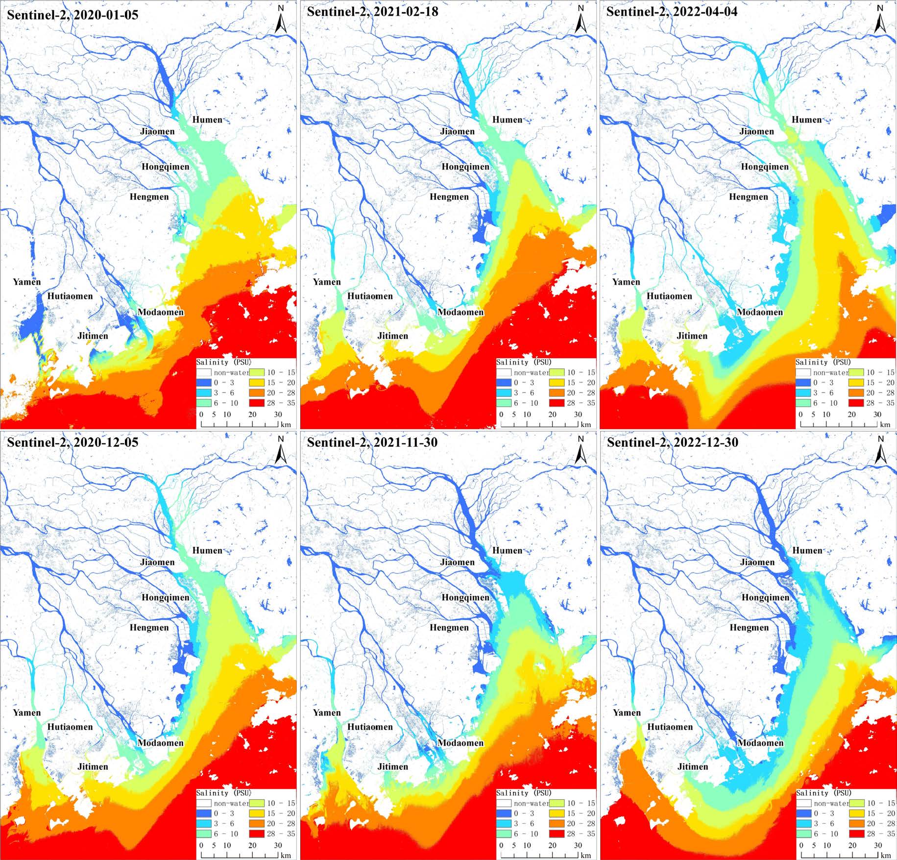
Satellite images with minimal cloud interference are chosen for both flood and ebb tides, guided by north-south tidal levels from four stations (Huangpu, Hengmen, Jiuzhou Port, Dawanshan), as shown in Figure 4. The ESS distribution for the corresponding date is depicted in Figure 5.

Tide curves for each tidal station at respective imaging times. Location information for the four tidal stations (blue: Huangpu, orange: Hengmen, gray: Jiuzhou Port, yellow: Dawanshan) can be found in Figure 1.
Generally, the ESS within the PRE shows a gradient with higher salinity in the southern regions decreasing towards northern areas and progressively diminishing from the open sea to the upstream river mouths. Various spatial distribution patterns emerge:
(1) During flood tides (Figure 5, first row: Dec. 5, 2020; Feb. 18, 2021; Apr. 4, 2022), tidal dynamics dominate the estuary. High-salinity eastern water intrudes and pushes upstream along deep river mouth channels, resulting in northward tongue-shaped salinity contours. Salinities in the eastern and central deep channels typically exceed those on the western shores. Salinity concentrations ranging from 3 to 6 PSU commonly extend to the Pearl River Front Channel and the East River North Branch.
(2) During ebb tides (Figure 5, second row: Jan. 5, 2020; Nov. 30, 2021; Dec. 30, 2022), downstream discharge dynamics dominate the estuary. Adjacent regions such as eastern Humen and western Jiaomen, along with Hongqimen, Hengmen, and Modaomen, become dominated by freshwater, with low-salinity outflows from upstream channels beyond the river mouths.

Sentinel-2 retrieval of ESS in the PRE at six different imaging times. Non-water pixels are excluded (white area). A color gradient from low (blue) to high (red), representing salinity values, is shown with a detailed distribution.
The obtained results above reveal that the remote sensing estimated salinity in the PRE exhibits significant spatial variability. To further visualize and quantify these errors, bias and RMSE maps for flood tides, ebb tides, and overall tidal periods are produced as shown in Figure 6. The first row of maps (Figure 6 a to Figure 6 c) depicts the bias, showing a positive bias (overestimation) in the salinity on the west coast of the estuary and upstream of Hengmen, with values ranging from 0 to 1 PSU during both flood and ebb tides. In contrast, the downstream open waters of the estuary exhibit a negative bias, with values ranging from -1 to -2 PSU.
The second row (Figure 6 d to Figure 6 f) represents the RMSE, which indicates that the overall riverine portion of the estuary exhibits an average error below 1.5 PSU. However, a slightly higher RMSE (1.5–2 PSU) is observed in the water body extending from northeast to southwest downstream of the PRE. This increased uncertainty may be attributed to two factors: the relatively sparse training data in this region and the complex interactions between freshwater input from rivers and ocean currents. Furthermore, during high tide, the bias and RMSE values are indeed higher than those observed during low tide. This might be due to the increased mixing of waters during high tide, leading to a more pronounced exchange of water between the river and the ocean. As a result, the remote-sensing estimated salinity may not accurately capture this dynamic process, resulting in larger errors. In contrast, during ebbing, the estuary’s water outflow tends to create more uniform salinity conditions, which leads to lower biases and errors in remote-sensing estimates.

Bias and RMSE maps of ESS estimated by remote sensing in the PRE. The top row shows the bias, with overestimation indicated by a blue-green color gradient and underestimation indicated by a yellow-red gradient. The bottom row illustrates the RMSE, with higher errors depicted in red and lower errors shown in blue.
DISCUSSION
By optimizing the input parameters, a practical algorithm for ESS estimation from Sentinel-2 imagery was proposed and applied to the PRE, a region notable for its high salinity variability resulting from the intricate ocean-estuary-runoff interaction.
Estuaries, where freshwater rivers meet the ocean, are among the most productive and biodiverse ecosystems on Earth. They are also highly vulnerable to human impacts, including land use changes, pollution, and climate-driven alterations in ocean circulation patterns. This is particularly true for estuaries like the PRE, whose unique geography, with its complex network of rivers, tidal flats, and mangrove forests, makes it especially susceptible to human activities and climate change impacts. To address these challenges, it is essential to develop accurate and effective monitoring strategies that can keep up with the complexity and variability of estuarine systems. This includes integrating data from multiple sources, such as satellite imagery, sensor networks, and hydrological models, to provide a comprehensive understanding of the PRE’s hydrodynamics and water quality, and the impacts of human activities on these processes.
Data analysis indicates that the PRE will experience low water flow from 2019 to 2028, a condition expected to intensify tidal intrusion (Yang et al., 2021). It poses a significant threat to the water supply security of coastal cities in the GBA and the ecological balance of the Pearl River Delta. Notably, the East River Delta of the PRE had a record-breaking saltwater intrusion during the dry season of 2021-2022, aligning with this predicted trend (Yang et al., 2023). This study aims to accomplish spatially continuous observation of water salinity in the PRE. To this end, satellite remote sensing technology distinguished by its expansive coverage and spatial continuity was chosen as the primary monitoring method. Despite the fact that Sentinel-2 has fewer spectral bands and broader spectral ranges compared to conventionally utilized ocean color satellites, the higher spatial resolution enhances its suitability for monitoring estuarine salt intrusion, thereby increasing the effectiveness of remote sensing. Although there is a disparity when juxtaposed against satellite data, even with enhanced resolution, Sentinel-2’s extensive coverage area (requiring merely two tiles to encompass the PRE region), coupled with the advantage of being freely accessible, led to our decision to adopt it as the primary data source.
During this process, however, we encountered an inevitable challenge: the lack of spectral response from water surface salinity, which cannot be directly inverted with optical remote sensing data. In past research, two typical approaches were adopted. One involved identifying water color parameters sensitive to salinity, thus obtaining salinity indirectly; the other entailed utilizing algorithms such as regression analysis, decision trees, neural networks, etc., to construct empirical models linking water surface salinity with various spectral combinations, selecting the model with the highest R² as the definitive salinity remote sensing model.
In the former approach, techniques have evolved from relying on a singular sensitive factor to applying multiple sensitive factors. Taking the PRE as an example, Chen et al. (2004) used colored dissolved organic matter (CDOM) as an indicator for salinity sensitivity, similar to other estuaries in Asia (Sasaki, et al., 2008), the Americas (Palacios et al., 2009) and Europe (Binding and Bowers, 2003). In high-salinity waters far from the shore, CDOM typically dominates the water body’s spectrum. However, when using the model in nearshore waters, where salinity gradients change significantly, the optical effects of other water components, such as suspended particles and chlorophyll, are often overlooked, which can lead to inconsistencies in the model results. More recently, He et al. (2020) suggested using suspended particulate matter during the flood season and the permanganate index and chlorophyll during the dry season. Nevertheless, fluctuations in proxy parameters frequently result in discontinuities within the spatial distribution of the salinity inversion results, hindering accurate comprehension of the salinity dynamics in other PRE regions.
In the latter approach, current investigations typically confine their scope to single-outlet estuaries, as shown by Jiang et al. (2024) focusing on the Modaomen of the PRE. Since simple linear or nonlinear equations are insufficient to describe the complex salinity distribution in multi-outlet estuaries, most researchers opt for neural networks. However, even with these advanced models, significant challenges arise from complex hydrodynamic factors (including tidal interactions, flooding and drying cycles, and a dense river network) and human activities. When relying solely on spectral information for surface salinity retrieval, significant errors may arise between retrieved and actual salinity values.
After analyzing the spatial distribution of the ESS, we discerned the basic pattern of salinity gradually decreasing from the estuary to the sea. Based on this revelation, we aimed to incorporate geographic information (i.e., the longitude and latitude of image pixels) as one of the input parameters, along with image spectral data for the ESS inversion. Ensuing model training and validation, we achieved high accuracy and obtained more uniform outcomes of salinity inversion.
Apart from spatial distribution traits, estuarine salinity is also subject to fluctuations in upstream water discharge from each estuary mouth, exhibiting temporal distribution attributes. To enhance the model’s practicality, we used the imaging date of the remote sensing images as another important parameter to reflect changes in upstream water flow and incorporated it into the model construction. The results displayed in Figure 5 also show that the model can capture the temporal variations in water surface salinity.
However, when constructing remote sensing models, it is crucial to acknowledge the fundamental distinction between site measurements and remote sensing images, namely, the difference between a point and an area. A point refers to a limited observational perspective yet with increased precision, whereas an area denotes a more expansive view that includes additional details or anomalies. Precisely due to this distinction, the process of model construction and analysis still has limitations and areas for improvement:
(1) Including geodetic coordinates enhances model physical mechanisms and accuracy, but may also cause overfitting. For example, N1G has the highest R2 according to Table 2, but N1G-01 and N1G-02 with ~0.95 R2 yield unreasonable results. As shown in Figure 6, abnormal 15–20 PSU in the Lingdingyang or negative upstream salinity on Jan. 5, 2020; N1G-02 also shows unrealistic phenomena like Modaomen high salinity upward movement and sudden Lingdingyang decrease. Future improvements could expand synchronized measurements for uniform estuary distribution, and refine input parameter weighting of neural network models.
(2) ESS distribution is significantly influenced by tides and upstream inflows. Figure 8 shows a comprehensive overview of this phenomenon based on salinity monitoring stations located near the Modaomen in the downstream PRE. Figure 8 a shows the tide level curves and corresponding salinity over a three-day period during a particularly severe saltwater intrusion in the winter of 2020. Figure 8 b provides a scatter plot of tide levels versus salinity during the same period. These figures reveal a positive correlation between tide levels and salinity, suggesting that, as the tide rises, high-salinity water from the sea intrudes upstream, increasing regional water salinity. During this period, the upstream West River flow was relatively low (approximately 3,200 m³/s), weakening the influence of river discharge on the regional hydrodynamic environment. In contrast, Figure 8 c depicts the tidal level and corresponding salinity during the flood season of the following year (2021), when the upstream West River discharge was significantly higher (around 14,800 m³/s). As expected, the impact of river runoff on local hydrodynamic conditions far surpassed that of tidal forces, leading to a notable decrease in water salinity and a weakened correlation between salinity and tide levels. Figure 9 presents data from Humen upstream during a severe saltwater intrusion at the end of 2021. Compared to Modaomen, the correlation between tidal level and salinity has increased significantly and exhibits a nonlinear relationship. This highlights the significant impact of both tidal cycles and river runoff on regional water salinity and underscores the spatial variability in salinity distribution within this complex estuary. To balance the mechanism and the practicality of remote sensing models, this study reduced input sources and used remote sensing image dates to represent estuary seasons and tides, which has certain limitations. Future improvements could incorporate upstream river flow data, like the West and East Rivers, to further enhance model accuracy and robustness.

Relationship between tide levels and salinity of the Modaomen in the downstream PRE. The top row shows the relationship over a three-day period during saltwater intrusion in the winter of 2020 by comparing tide level curves with concurrent salinity (a), and the corresponding scatter plot (b). The bottom row depicts the varied relationship during flood season in the following year by curves comparison (c) and scatter plot (d).

Relationship between tide levels and salinity of Humen in the upstream PRE during Saltwater Intrusion Events. The left plot (a) shows that the correlation between tidal level and salinity has increased significantly, while the right plot (b) exhibits a nonlinear relationship compared to Modaomen areas.
CONCLUSIONS
This study utilizes extensive historical imagery and synchronized salinity measurement to construct a neural network-based remote sensing method for ESS applicable to Sentinel-2 imagery. The neural network model demonstrates strong nonlinear fitting capabilities, achieving effective inversion in the PRE with complex tidal-river interaction and multi-gate hydrology. The ESS in the PRE exhibits higher southern and lower northern spatial patterns, with outer estuary areas higher than inner ones, influenced by tidal dynamics. Incorporating longitude/latitude for spatial information and dates for tidal information enhances the ESS model’s physical mechanism. Spectral processing, like near-infrared correction and band ratios, further improves model precision and stability. The inversion revealed high-salinity seawater coming from the eastern channel during flood tides, gradually merging upstream with freshwater. Low-salinity masses reached the Front Channel of the Pearl River and the North Branch of the East River. During ebb tides, due to downstream runoff, the low-salinity mass surged outwards, primarily retreating eastward to Humen.
Data availability statement
The measured salinity are not publicly available due to commercial confidentiality agreements. However, the remote sensing data used in this study can be accessed through publicly available online platforms. Sentinel-2 images can be obtained from the Copernicus Browser (https://browser.dataspace.copernicus.eu/).
Supplementary material
No supplementary material is provided.
Funding
The Guangdong Provincial Water Resources Science and Technology Innovation Project (2023-01); the Ministry of Water Resources Major Science and Technology Project (SKS-2022005).
Acknowledgments
The authors acknowledge the projects supported by the following grants: the Guangdong Provincial Water Resources Science and Technology Innovation Project (2023-01) “Research on Salinity Monitoring, Forecasting, and Control Strategies in the Pearl River Estuary,” the Ministry of Water Resources Major Science and Technology Project (SKS-2022005) “Key Technologies and Control Strategies for Identifying Salinity Risks in the Pearl River under Extreme Drought,” and the Science and Technology Innovation Independence Project of Pearl River Water Resources Research Institute ([2023]YF005). These projects have provided invaluable resources, data, and technical support, enabling us to delve into the satellite monitoring of salinity intrusion in the Pearl River Estuary, and making solid strides on our scientific journey.
The authors also extend their gratitude to the OCR editors and reviewers for their patient guidance and assistance in optimizing this work.
REFERENCES
-
Binding C. E., Bowers D. G., 2003. Measuring the salinity of the Clyde Sea from remotely sensed ocean colour. Estuarine, Coastal and Shelf Science, 57(4): 605-611. DOI: https://doi.org/10.1016/S0272-7714(02)00399-2
» https://doi.org/10.1016/S0272-7714(02)00399-2 -
Cao Bin, Qiu Zhenge, Cao Bincai, 2017. lmprovement of BPANN Based Algorithm for Estimating Water Depth from Satellite Imagery. Bulletin of Surveying and Mapping 5. DOI: ( https://doi.org/10.13474/j.cnki.11-2246.2017.0045 )
» https://doi.org/10.13474/j.cnki.11-2246.2017.0045) -
Chen, S., Hu, C., 2017. Estimating sea surface salinity in the northern Gulf of Mexico from satellite ocean color measurements. Remote Sensing of Environment 201, 115–132. DOI: ( https://doi.org/10.1016/j.rse.2017.09.004 )
» https://doi.org/10.1016/j.rse.2017.09.004) -
Chen, Z., Li, Y., Pan, J., 2004. Distributions of colored dissolved organic matter and dissolved organic carbon in the Pearl River Estuary, China. Continental Shelf Research 24, 1845–1856. DOI: ( https://doi.org/10.1016/j.csr.2004.06.011 )
» https://doi.org/10.1016/j.csr.2004.06.011) -
Hagan M.T., M. Menhaj., 1999, Training feed-forward networks with the Marquardt algorithm. IEEE Transactions on Neural Networks, 5(6), 989-993. DOI: https://doi.org/10.1109/72.329697 .
» https://doi.org/10.1109/72.329697 -
He, Y., Gong, Z., Zheng, Y., Zhang, Y., 2021. Inland Reservoir Water Quality Inversion and Eutrophication Evaluation Using BP Neural Network and Remote Sensing Imagery: A Case Study of Dashahe Reservoir. Water 13, 2844. DOI: https://doi.org/10.3390/w13202844
» https://doi.org/10.3390/w13202844 -
He Yingqing, Feng Youbin, Fu Qinghua, Liu Chaoqun, 2020. A Study on Optical Remote Sensing Inversion of Sea Surface Salinity in the Pearl River Estuary. Geography and Geo-Information Science 36(6), 40-47. DOI: https://doi.org/10.3969/j.issn.1672-0504.2020.06.007
» https://doi.org/10.3969/j.issn.1672-0504.2020.06.007 -
Jiang, D., Dong, C., Ma, Z., Wang, X., Lin, K., Yang, F., Chen, X., 2024. Monitoring saltwater intrusion to estuaries based on UAV and satellite imagery with machine learning models. Remote Sensing of Environment 308, 114198. https://doi.org/10.1016/j.rse.2024.114198
» https://doi.org/10.1016/j.rse.2024.114198 -
Kim, Y.J., Han, D., Jang, E., Im, J., Sung, T., 2023. Remote sensing of sea surface salinity: challenges and research directions. GIScience & Remote Sensing 60, 2166377. DOI: https://doi.org/10.1080/15481603.2023.2166377
» https://doi.org/10.1080/15481603.2023.2166377 -
Kolodziejczyk, N., Boutin, J., Vergely, J.-L., Marchand, S., Martin, N., Reverdin, G., 2016. Mitigation of systematic errors in SMOS sea surface salinity. Remote Sensing of Environment, Special Issue: ESA’s Soil Moisture and Ocean Salinity Mission - Achievements and Applications 180, 164–177. DOI: https://doi.org/10.1016/j.rse.2016.02.061
» https://doi.org/10.1016/j.rse.2016.02.061 -
Liu, R., Zhang, J., Yao, H., Cui, T., Wang, N., Zhang, Y., Wu, L., An, J., 2017. Hourly changes in sea surface salinity in coastal waters recorded by Geostationary Ocean Color Imager. Estuarine, Coastal and Shelf Science 196, 227–236. DOI: https://doi.org/10.1016/j.ecss.2017.07.004
» https://doi.org/10.1016/j.ecss.2017.07.004 -
Sentinel-2 MPC Team. Sentinel-2 Level-2A Algorithm Theoretical Basis Document (S2-PDGS-MPC-ATBD-L2A). 15 Nov. 2021]; Available from: https://step.esa.int/thirdparties/sen2cor/2.10.0/docs/S2-PDGS-MPC-L2A-ATBD-V2.10.0.pdf .
» https://step.esa.int/thirdparties/sen2cor/2.10.0/docs/S2-PDGS-MPC-L2A-ATBD-V2.10.0.pdf -
Nakada, S., Kobayashi, S., Hayashi, M., Ishizaka, J., Akiyama, S., Fuchi, M., Nakajima, M., 2018. High-resolution surface salinity maps in coastal oceans based on geostationary ocean color images: quantitative analysis of river plume dynamics. J Oceanogr 74, 287–304. DOI: https://doi.org/10.1007/s10872-017-0459-4
» https://doi.org/10.1007/s10872-017-0459-4 -
Palacios S. L., Peterson T. D., Kudela R. M., 2009. Development of synthetic salinity from remote sensing for the Columbia River plume. Journal of Geophysical Research: Oceans, 114(C2). DOI: ( https://doi.org/10.1029/2008JC004895 )
» https://doi.org/10.1029/2008JC004895) -
Reul, N., Grodsky, S.A., Arias, M., Boutin, J., Catany, R., Chapron, B., D’Amico, F., Dinnat, E., Donlon, C., Fore, A., Fournier, S., Guimbard, S., Hasson, A., Kolodziejczyk, N., Lagerloef, G., Lee, T., Le Vine, D.M., Lindstrom, E., Maes, C., Mecklenburg, S., Meissner, T., Olmedo, E., Sabia, R., Tenerelli, J., Thouvenin-Masson, C., Turiel, A., Vergely, J.L., Vinogradova, N., Wentz, F., Yueh, S., 2020. Sea surface salinity estimates from spaceborne L-band radiometers: An overview of the first decade of observation (2010–2019). Remote Sensing of Environment 242, 111769. DOI: ( https://doi.org/10.1016/j.rse.2020.111769 )
» https://doi.org/10.1016/j.rse.2020.111769 -
Sasaki H., Siswanto E., Nishiuchi K., Tanaka K., Hasegawa T., Ishizaka J., 2008. Mapping the low salinity Changjiang Diluted Water using satellite-retrieved colored dissolved organic matter (CDOM) in the East China Sea during high river flow season. Geophysical Research Letters, 35(4). DOI: https://doi.org/10.1029/2007GL032637
» https://doi.org/10.1029/2007GL032637 -
Taillade, T., Engdahl, M., Fernandez, D., 2023. Can We Retrieve Sea Surface Salinity With Polarimetric Radar Measurements? IEEE Geoscience and Remote Sensing Letters 20, 1–5. DOI: https://doi.org/10.1109/LGRS.2023.3286436
» https://doi.org/10.1109/LGRS.2023.3286436 -
Urquhart, E.A., Zaitchik, B.F., Hoffman, M.J., Guikema, S.D., Geiger, E.F., 2012. Remotely sensed estimates of surface salinity in the Chesapeake Bay: A statistical approach. Remote Sensing of Environment 123, 522–531. DOI: https://doi.org/10.1016/j.rse.2012.04.008
» https://doi.org/10.1016/j.rse.2012.04.008 -
Wang, J., Sun, W., Zhang, J., 2019. Sea Surface Salinity Products Validation Based on Triple Match Method. IEEE Journal of Selected Topics in Applied Earth Observations and Remote Sensing 12, 4361–4366. DOI: https://doi.org/10.1109/JSTARS.2019.2945486
» https://doi.org/10.1109/JSTARS.2019.2945486 - Yang F., Lin Z., Zou H., Zhu L., Zou X., 2023. Study on the response law of saltwater intrusion in the Dongjiang Delta of the Pearl River Estuary under extreme drought conditions. Marine Science Bulletin 42, 496–507.
-
Yang Fang, He Yingqing, Lu Chen, Zou Huazhi, 2021. Changes of seawater invention situation in the Pearl River estuary and salinity reduction solutions. China Water Resources 5, 21–23. DOI: https://doi.org/10.3969/j.issn.1000-1123.2021.05.012
» https://doi.org/10.3969/j.issn.1000-1123.2021.05.012 -
Zhang, L., Zhang, R., He, Q., 2020. Sea Surface Salinity Retrieval from Aquarius in the South China Sea Using Machine Learning Algorithm, in: IGARSS 2020 - 2020 IEEE International Geoscience and Remote Sensing Symposium. Presented at the IGARSS 2020 - 2020 IEEE International Geoscience and Remote Sensing Symposium, pp. 5643–5646. DOI: ( https://doi.org/10.1109/IGARSS39084.2020.9323153 )
» https://doi.org/10.1109/IGARSS39084.2020.9323153 -
Zhang, L., Zhang, Y., Yin, X., 2023. Aquarius sea surface salinity retrieval in coastal regions based on deep neural networks. Remote Sensing of Environment 284, 113357. https://doi.org/10.1016/j.rse.2022.113357
» https://doi.org/10.1016/j.rse.2022.113357 -
Zhang, Z., Cui, B., Zhao, H., Fan, X., Zhang, H., 2010. Discharge-salinity relationships in Modaomen waterway, Pearl River estuary. Procedia Environmental Sciences, International Conference on Ecological Informatics and Ecosystem Conservation (ISEIS 2010) 2, 1235–1245. DOI: https://doi.org/10.1016/j.proenv.2010.10.134
» https://doi.org/10.1016/j.proenv.2010.10.134 -
Zhou, Y., Lang, R.H., Dinnat, E.P., Le Vine, D.M., 2017. L-Band Model Function of the Dielectric Constant of Seawater. IEEE Transactions on Geoscience and Remote Sensing 55, 6964–6974. DOI: https://doi.org/10.1109/TGRS.2017.2737419
» https://doi.org/10.1109/TGRS.2017.2737419
Edited by
-
Associate Editor:
Cesar Rocha