Real-time drifter tracking system for coastal studies

ABSTRACT

This article presents a real-time drifter tracking system designed to investigate circulation and transport processes in coastal environments. Field demonstrations were conducted in two contrasting Brazilian coastal regions: Florianópolis Island in the south, a microtidal area driven primarily by wind circulation, and São Marcos Bay in the northeast, an estuary complex characterized by strong tidal forcing. Surface Velocity Program (SVP) drifters were adapted for coastal applications, incorporating a reel to adjust drogue depth and electronic systems housed in a 3D-printed enclosure. The tracking system was also tested with an undrogued iSphere drifter to assess estuarine surface circulation. Satellite communication systems enabled real-time tracking for efficient deployment and recovery of drifters, while optional fast-response loggers ensured near-continuous data collection. Results revealed rapid circulation responses to wind forcing north of Florianópolis Island, and a tidal-dominated environment in São Marcos Bay, with secondary influence from wind and waves. The real-time tracking system prevented equipment loss and enhanced data acquisition. This reusable drifter setup offers a practical solution for oceanographic studies, supporting repeated deployments, streamlined data collection, and adaptability to various coastal applications and drifter types.

Keywords:
SVP drifter; iSphere; Coastal circulation; Florianópolis; São Marcos Bay

INTRODUCTION

Coastal circulation drives the transport of water masses, nutrients, and pollutants, playing a central role in the dynamics of marine ecosystems. Understanding these processes is crucial for human activities such as port operations, oil exploration, and the planning of sustainable coastal infrastructure.

Surface drifters are essential tools for studying circulation, providing accurate data on particle trajectories, flow velocities, and patterns. Modern drifters typically comprise a surface buoy, a submerged drogue, and electronic systems, including Global Navigation Satellite System (GNSS) receivers, communication modules, and environmental sensors (Lumpkin et al., 2017; Richardson, 2009). They are designed to be lightweight, durable, cost-effective, and easy to deploy. In many cases, drifters are programmed for periodic data transmission, with no intention of instrument recovery.

The Surface Velocity Program drifter (SVP), for example, was designed to track the mixed layer, with velocity measurements averaged vertically over a 6-m tall drogue centered at 15 m below the ocean surface (Niiler et al., 1991). The Global Drifter Program - part of the WOCE and TOGA - deployed thousands of SVP to resolve global ocean circulation and eddy energy at high spatial resolution (Lumpkin et al., 2017; Pazan, 2004).

Drifters were also used to investigate the continental shelf (Assireu et al., 2003; Griggs, 1974) and gulf circulation (Mariano et al., 2016), estuarine and bay exchange processes (Conomos et al., 1972; Pape and Garvine, 1982; Pawlowicz et al., 2019), coastal plume dynamics (Kakoulaki et al., 2020), circulation in shallow environments (Mullarney and Henderson, 2013), surf zone (Schmidt et al., 2003), and surface gravity waves (Guimarães et al., 2018).

Beyond scientific research, drifters were employed in various practical applications, including search and rescue operations (Breivik and Allen, 2008), tracking of plumes from ocean outfalls (Terrill et al., 2014), monitoring of plastic transport (Merlino et al., 2023), as well as studies of macroalgae drift and larval dispersal (Méndez-Jiménez et al., 2015).

In coastal environments, circulation is driven by complex factors, including astronomical tides, buoyancy, waves, wind forcing, and interactions with large-scale currents (Csanady, 1982). Unlike deep-water drifters, which use drogues without depth constraints, coastal drifters are restricted by shallower operating depths.

Previous studies focused on coastal surface circulation have utilized undrogued drifters, such as the “bucket-type” described by Kakoulaki et al. (2014) or the cylindrical PVC drifter reported by van der Mheen et al. (2020). Other studies concerned with the combined effects of surface currents and waves employed the CODE-Davis type of drifter, with a drogue consisting of a one-meter-long tube with four radial panels for drag (Davis, 1985; Tseng, 2002). Other applications employed drifters with drogues centered at 1 m depth, such as the Microstar drifter (Pacific Gyre, 2023; Subbaraya et al., 2016).

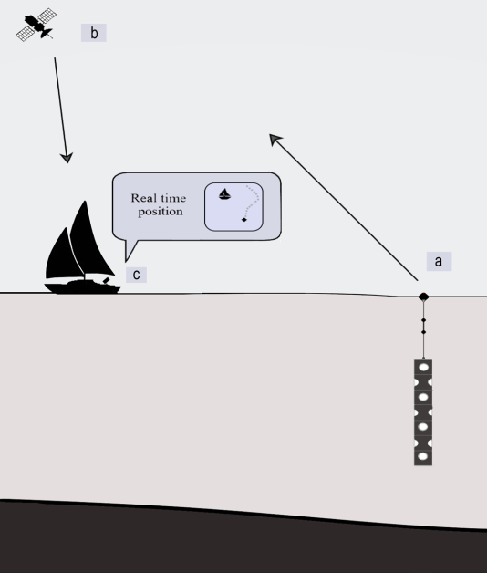
In this study, Surface Velocity Program (SVP) drifters were adapted to investigate coastal circulation by employing a fully extended, reduced-depth drogue to minimize the risk of stranding. The drifters also incorporated fast-response satellite positioning and communication systems. The aim was to adapt a robust deep-ocean drifter for shallow-water applications by designing a reel system to reduce the drogue depth. Specifically, the SVP drifters were used here to track the near-surface flow with a 6.2 m long drogue centered at approximately 6 m depth. Another key objective was to test a cost-effective, real-time tracking setup to streamline drifter deployment and recovery in coastal environments, with potential applications to other drifter types (Figure 1).

Figure 1
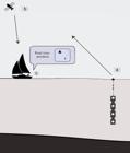
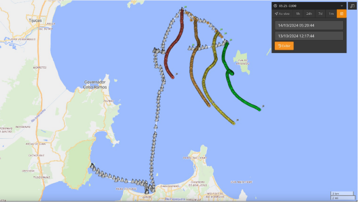
Real-time drifter tracking system. (a) The buoy transmits its position via satellite communication. (b) Starlink enables real-time communication, receiving buoy and vessel positions at short intervals, in support of deployment and recovery operations. (c) Navigation system provided by the FindMeSpot web service, showing the vessel and drifter positions.

Recoverable systems have been successfully used in previous studies, enabling repeated experiments and substantially reducing equipment costs. For instance, Schmidt et al. (2003) used radio frequency telemetry for tracking surf-zone drifters, while Kakoulaki et al. (2014, 2020) conducted multiple drifter deployments in the Merrimack River plume using a GPS satellite tracking system provided by Comtech Mobile Datacom. Assireu et al. (2026) employed drifters to measure the Doce River discharge using a GNSS receiver integrated with a cellular modem. However, the proposed system has nearly worldwide satellite coverage, facilitating its application across diverse aquatic environments.

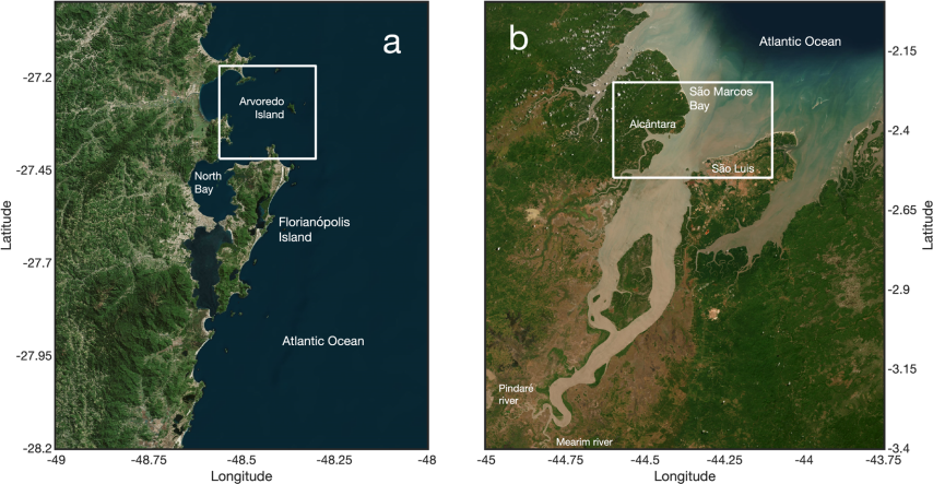
The coastal SVP drifters and their tracking system were tested in two distinct oceanographic environments along the Brazilian coast. The first site lies north of Florianópolis Island and southwest of Arvoredo Island, a region characterized by a microtidal regime, predominantly wind-driven circulation, and depths ranging from 10 to 50 m (Dalbosco et al., 2020; Pimenta et al., 2004) (Figure 2a).

Figure 2
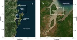
(a) Florianópolis Island in southern Brazil. The study area is in the northern part of Florianópolis and southwest of Arvoredo Island. (b) São Marcos Bay in northeastern Brazil. The study region is situated between Alcântara and São Luís.

The second site, São Marcos Bay, between Alcântara and São Luís in Maranhão, northeastern Brazil, features macrotidal ranges, low river discharge, steady wind forcing, and depths of 10-50 m (Czizeweski et al., 2020; El-Robrini et al., 1992) (Figure 2b). In São Marcos, the tracking system was also tested with an iSphere drifter (MetOcean, 2017). This type of drifter is undrogued and commonly used for oil spill tracking (Ivichev et al., 2012; Woodbury, 2017), but in this study it was employed to monitor surface currents in the uppermost layer and to compare its behavior with that of drogued SVP drifters.

This article is organized into three main sections. The next section details the methods, including drifter adaptations (drogue-cable reducer and electronic equipment enclosure), drag force calculations, satellite tracking and communication systems, and rescue procedures. The third section shows experimental results from deployments conducted in October 2024 off Florianópolis Island and in April 2025 in São Marcos Bay, highlighting deployment and recovery strategies as well as observed circulation patterns. The final section provides a summary and concluding remarks.

METHODS

DRIFTER ADAPTATIONS

The SVP drifters used in this study were provided by the National Oceanic and Atmospheric Administration (NOAA) via the Brazilian Navy’s PNBOIA Program. Seven SVP drifters were adapted for coastal applications by shortening the drogue cable. A protective shelter was also designed to house new satellite tracking electronics and enhance the buoy’s signaling for rescue operations. Moreover, one undrogued iSphere drifter hull was employed to compare with the SVP drifters, and to test the proposed tracking system.

DROGUE-CABLE REEL

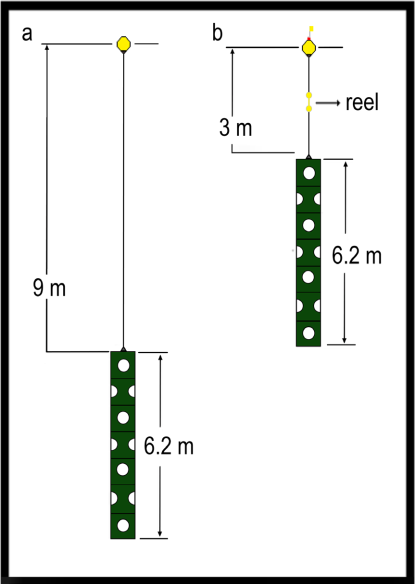
Surface Velocity Program (SVP) drifters were originally designed for deep-ocean applications, with 6.2-m-long drogues positioned at 15 m depth, reaching a maximum depth of approximately 18 m (Figure 3a). With this configuration, the drag ratio of the drogue to its cable and submerged buoy is 38:1, such that the buoy responds primarily to so-called “mixed layer currents”, being suitable for deep-water, outer, and mid-continental shelf studies (Niiler et al., 1991).

Figure 3
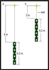
(a) Original configuration of the Surface Velocity Program (SVP) drifter, with a full cable length of 9 m and a drogue of 6.2 m, designed for deep-ocean applications. (b) Coastal SVP drifter adapted for shallower waters, with the drogue-cable length reduced to 3 m using a reel.

In this study, SVP drifters were adapted for shallower environments, such as bays and inner- to mid-shelf regions. The primary modification involved designing a reel system to adjust the cable length without cutting, enabling the drogue to be positioned closer to the surface or at mid-depth.

The concept of varying drogue depth is not new. Krauss (1993) used satellite-tracked cylindrical buoys with 10-m holey-sock drogues to track different water layers in the Yellow Sea, with positions obtained via the Argos system six to eight times daily (every three to four hours). Geyer (1989) employed holey-sock drifters with varying buoy and drogue diameters, tracked by the del Norte microwave positioning system, in coastal waters of 12-20 m depth to quantify drifter performances.

In contrast, the proposed setup incorporates a reel mechanism for customizable drogue depth adjustments, tailored to specific environmental conditions and applications. Furthermore, the integration of new tracking technologies enhances deployment and recovery efficiency while improving temporal and spatial resolution, as detailed in subsequent sections.

Figure 3b illustrates the layout of the adapted SVP drifter, highlighting the reel for cable length adjustment. In our application, the cable was shortened to 3 m, positioning the drogue to a maximum depth of 9.2 m. This restricts the drifter’s application to depths of approximately 12 m. The drogue spans a significant portion of the upper water column, and the drifter’s response is representative of the near-surface flow.

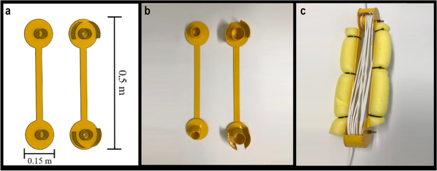
The reel consists of two 0.5-m long, 0.15-m wide steel sections, with cylindrical pivots and broad lateral protections to guide the cable (Figure 4a). The cable can be wound in a “figure-eight” pattern, enabling shortening to the desired depth before deployment. The reel was coated with yellow paint to enhance visibility (Figure 4b). Two bolts with nuts connect the two sections, and once assembled, foam spaghetti tubes can be attached to counterbalance the reel’s weight (Figure 4c).

Figure 4
Reel design and complete assembly for cable-length reduction. (a) CAD design with part dimensions; (b) photograph of the disassembled steel reel; (c) photograph of the assembled reel with cable and floaters to neutralize its weight in water.

ELECTRONICS PROTECTIVE SHELTER

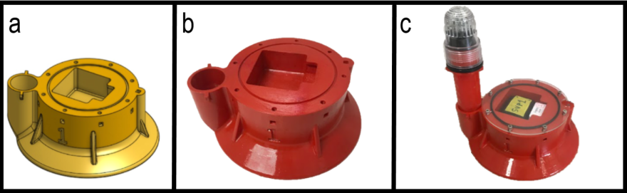
A protective shelter for electronic components was designed with OnShape software for installing the electronics on the top of SVP buoys. The shelter was fabricated via 3D printing with PETG filament, chosen for its high impact resistance and thermal stability. The shelter features a central compartment to house electronic sensors and is reinforced around its perimeter with ribs for increased rigidity. The base was designed to be wide and rounded for secure mounting on the SVP surface buoy. Two laterally reinforced spaces were incorporated to accommodate LED light and a flag mast (Figure 5a).

Figure 5
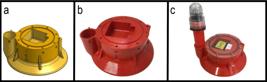
Tracker device shelter. (a) CAD design of the shelter. (b) 3D-printed shelter using PETG filament. (c) Finished shelter with epoxy resin coating, sensors, LED light, flag mount, acrylic lid, screws, and O-ring.

After printing, the shelter was laminated with epoxy resin to ensure waterproofing and increased mechanical strength, crucial for withstanding harsh marine conditions (Figure 5b). The shelter was securely attached to the buoy with silicone glue, and the final assembly included an acrylic lid secured with eight socket head Allen bolts and a sealing O-ring, ensuring watertightness.

Special inserts were designed to accommodate rectangular nuts for firmly tightening the lid. Figure 5c shows the shelter mounted with sensors, acrylic lid, O-ring, bolts, and the signaling LED light to facilitate drifter signaling in dark hours (Kakoulaki et al., 2020).

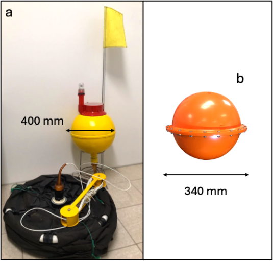
Figure 6a illustrates the coastal SVP drifter assembled for deployment, with its electronics shelter, flag, and light installed, cable shortened by the reel, and drogue secured with ropes for transport. The electronics shelter, installed facing upward, is a mandatory requirement for electronics onboard. Figure 6b illustrates the undrogued iSphere, with a 34 cm diameter. An empty buoy hull was equipped with a Spot Trace tracker and rebalanced with lead to maintain the waterline at the design level.

Figure 6
(a) Coastal SVP drifter setup, featuring a cable reduction reel, shelter for housing electronics, signaling light, flag, and its drogue. (b) iSphere undrogued drifter.

DRIFTER DRAG FORCES AND DOWNWIND SLIP

Winds acting on the drifter’s surface generate drag that induces slip aligned with the wind direction. Similarly, submerged components, such as the buoy and cable, experience additional forces due to the combined effects of winds and waves that are confined near the surface (Niiler et al., 1995).

Given the complexity of modeling these combined forces, field measurements have been conducted to quantify drifter’s relative response to wind. Geyer (1989) employed holey-sock drifters and a drifting current meter array to obtain estimates of slip velocity that varied between 1 and 4 cm s^-1. Niiler et al. (1995) installed vector-averaging current meters at the top and bottom of SVP drifter holey-sock drogues and estimated the downwind slip to be on the order of Us≈0.001 Uw, where Uw is the wind speed.

Poulain and Gerin (2019) used Aquadopp acoustic velocimeters mounted on CODE/Davis-type drifters to estimate a slip of about 0.1% of the wind speed. Pawlowicz et al. (2024) simultaneously deployed drogued and undrogued drifter types alongside rhodamine dye in a field experiment designed to assess their water-tracking performance. Notably, the undrogued iSphere had the largest downwind slip of approximately Us≈0.04 Uw, equivalent to 4% of the wind speed.

Following the modifications to the coastal SVP drifter design, it is worthwhile to reassess the influence of wind and currents on its components. Table 1 lists the lengths (L), diameters (D), areas (A), drag coefficients (Cd), and drag areas (Cd A) for the different components of the coastal SVP. It also evaluates drag forces for emerged and submerged components of the drifter under strong winds of 10 m s^-1 and ocean currents of 0.5-2.0 m s^-1. Drag forces are computed using the quadratic drag formula, which accounts for fluid density, drag area and the square of the relative fluid velocity.

Table 1
Drag areas and forces on coastal SVP drifter components. Drag forces are computed separately for emerged parts under 10 m s^-1 winds and submerged parts under 0.5-2.0 m s^-1 currents. Here L represents the length (cm), D the diameter (cm), and Cd represents the drag coefficients, following Niiler et al. (1991), Niiler et al. (1995) and Cengel and Cimbala (2011). Frontal area A (m²) is calculated from A=LD (after converting units) for most components, A=LD/2 for urethane (cone projection), A=(πD²)/4 for the spherical buoy (half disk), and A=LD for the flag, representing a plate aligned with the wind. (Cd A) represents the drag area.

Surface drifter components	L (cm)	D (cm)	A (m2)	Cd	Cd A	Drag force (N) from 10 m s-1 winds
Tracker shelter	10	15	0,0150	0,600	0,0090	0,54
Flag	20	15	0,0600	0,010	0,0006	0,04
Aluminum square mast	65	0,8	0,0052	2,200	0,0114	0,69
Lantern	26	4,8	0,0125	0,820	0,0102	0,61
Surface buoy (emerged)	-	40	0,0628	0,500	0,0314	1,88
Total					0,0627	3,76
Subsurface drifter components						Drag force (N) from currents
						0.5 m s-1	2.0 m s-1
Surface buoy (submerged)	-	40	0,0628	0,500	0,031	4,03	64,40
Buoy urethane connection	40	4	0,0080	1,000	0,008	1,03	16,40
Cable	300	1	0,0300	1,400	0,042	5,38	86,10
2 reel disks	-	15	0,0353	1,000	0,035	4,53	72,45
Reel axis	50	2	0,0100	1,300	0,013	1,67	26,65
Spaghetti float	30	6	0,0180	0,800	0,014	1,85	29,52
Drogue urethane connection	40	4	0,0080	1,000	0,008	1,03	16,40
Drogue	620	60	3,7200	1,400	5,208	667,28	10676,40
Total					5,360	686,77	10988,33
Ratio subsurface/surface					85,50	182,59	2921,36
Ratio drogue/(buoy+cables)					36,18	36,18	36,18

The emerged components-tracker shelter, flag, mast, lantern, and surface buoy generate an expected drag (Fw) of 3.8 N for winds of 10 m s^-1. In contrast, submerged components, including the buoy, cable, reel, spaghetti float, and drogue, produce an estimated current drag (Fc) that ranges from 687 N to 10988 N. The Fc/Fw ratio, ranging from 183 to 2921, highlights the dominance of current-induced drag, particularly from the drogue, emphasizing the drifter’s dominant response to ocean currents.

The drogue and its urethane connection contribute most of the submerged drag, compared to other submerged components (surface buoy, buoy urethane connection, cable, reel, and spaghetti float). This results in a drag ratio of 36.2, slightly lower than the original SVP drogue-to-cable ratio of 38 for deep-water drifters (Niiler et al., 1991), yet it indicates that the coastal SVP drifter remains responsive to currents acting on the drogue.

As the addition of surface components increase the wind drag over the coastal SVP, it is worthwhile to estimate the impact of these elements through a simplified drag balance of its surface and subsurface components. Assuming a steady drag balance between air acting on exposed components and water acting on submerged components, the resulting downwind slip can be estimated as (Kirwan, 1975; Poulain & Gerin, 2019):

$U_s=\sqrt{\frac{{\rho }_a}{{\rho }_w}\frac{\Sigma {\left(C_{d}A\right)}_a}{\Sigma {\left(C_{d}A\right)}_w}}{U}_w$

with the air density (1.2 kg m^-3) and as the water density (1025 kg m^-3). According to Table 1, here and represent the sum of surface and submerged drag areas, respectively. This expression, if applied to the classical SVP (=8.52 m², 0.024 m²) results in Us≈0.0018 Uw for a drogue of 92 cm of diameter (Niiler et al., 1991). The additional surface components increase wind drag influence, corresponding to Us≈0.0037 Uw for our 60 cm diameter drogue.

For the iSphere buoy, the emerged part would generate near 1.36 N of drag for wind of 10 m s^-1, while the submerged part produces 2.91 N to 46.53 N for currents of 0.5-2.0 m s^-1, yielding an Fc/Fw ratio that varies from 2.1 to 34.2. The same simplified wind drag analysis, when applied to the iSphere, can be expressed as $U_s~\sqrt{{\rho }_s/{\rho }_w}{U}_w$, what results in Us≈0.034 Uw, one order of magnitude larger than the coastal SVP estimated downwind slip.

SATELLITE COMMUNICATION AND POSITIONING

The integration of satellite tracking and communication systems is a crucial component in the study of recoverable coastal drifters, as it enables trajectory data acquisition and real-time monitoring. Two off-the-shelf tracking devices were used on our buoys (Spot Trace and i-gotU GT-600B), complemented by a Starlink communication system installed on the vessel (Figure 7).

Figure 7
Satellite-based tracking and communication systems: (a) Spot Trace for real-time drifter position tracking; (b) Starlink for high-speed satellite communication at sea; (c) i-gotU data logger for high-accuracy geographic position recording.

The Spot Trace is an asset tracker developed by Globalstar, commonly used for boats and high-value cargo. In this study, the device was employed to track the position of the buoy, using the Globalstar satellite communication network, which offers low latency and near-global coverage with position reporting at programmable intervals.

The use of Spot Trace in drifter applications is not new, it has been successfully employed in previous coastal (e.g., Pawlowicz et al., 2019), shelf (Morey et al., 2018), and deep-ocean deployments (Siji and Pattiaratchi, 2025, van Sebille et al., 2021). The GLAD experiment, for example, deployed 297 CODE-style drifters equipped with Spot Trace units to study surface velocity statistics and dispersion processes in the Gulf of Mexico (Mariano et al., 2016). More than 1,000 biodegradable drifters equipped with Spot Trace were used in the Lagrangian Submesoscale Experiment (LASER) (Lumpkin et al., 2017; Novelli et al., 2017).

This equipment measures 68.3 mm in length, 51.3 mm in width, and 21.44 mm in thickness, weighing 87.9 g (Figure 7a). The device includes a vibration sensor to detect movements, combined with a GPS and communication system. Globalstar recommends four AAA lithium batteries for optimal performance, though alkaline batteries were used in our fieldworks. Table 2 specifies that the equipment can be set to a sampling rate between 2.5 to 60 minutes, which results in battery autonomy that varies from six to 60 days.

Table 2
Spot Trace autonomy and tracking.

Spot Trace
Transmission interval Δt	Battery life (constant movement)	Drift distance (m) at Δt
		0.25 m s-1	0.5 m s-1	2 m s-1
60 min	60 days	900 m	1800 m	7200 m
30 min	35 days	450 m	900 m	3600 m
15 min	20 days	225 m	450 m	1800 m
10 min	13 days	150 m	300 m	1200 m
5 min	8 days	75 m	150 m	600 m
2½ min	6 days	37.5 m	75 m	300 m

Spot Trace also has a line-power option with a 5V USB connection, but this was not used due to the short duration of our campaigns. The device was configured with “dock mode disabled” during field operations. The tracker can enter sleep mode if no movement or vibration occurs, a situation that may arise during very low waves and negligible currents. To prevent this, the device shelter was designed with extra space around the equipment to enable movement inside the shelter. Although the sensor has an IP68 rating, it was protected with a ziplock bag.

The Spot Trace must be positioned face-up to ensure effective Iridium satellite communication (Figure 5c). Previous studies report positioning standard errors of 2.5 to 6 m (Lumpkin et al., 2017; Pawlowicz et al., 2019), with 95% of positions having an error of 10 m or less (Novelli et al., 2017). The ability to transmit real-time alerts every 2.5 minutes is essential for locating drifters during rescue operations, reducing the chance of equipment loss.

The Starlink satellite communication system (Figure 7b) enables continuous monitoring of drifters during the deployment and recovery phases by providing internet access to the Globalstar FindMeSpot web portal (Figure A1). Through this portal, drifter positions, reported by Spot Trace, can be accessed in near real-time, so that the tracking history can be plotted on a map.

The system also provides a reliable communication link that can be powered by a solar panel, battery, and inverter, making it particularly valuable in regions where rescue operations are often conducted using opportunistically rented vessels. During our field operations, an additional Spot Trace device was installed on the vessel, serving as a point of reference for navigation via the FindMeSpot mapping system (Figure A1).

The i-gotU (model GT600B), a high-sensitivity data logger, records position, velocity, at intervals ranging from one to 60 seconds, with a battery life of 40 hours at one-second intervals to 400 hours at 60-second intervals (Table 3). Measuring 46 mm in height, 41.5 mm in width, and 14.3 mm in thickness, and weighing 33 g, the device must also be installed facing upward to optimize satellite reception (Figure 7c). It also incorporates a vibration sensor to conserve power.

Table 3
I-gotU transmission range, drift distance, and autonomy.

i-gotU
Recording interval Δt	Battery life (constant movement)	Drift distance (m) at Δt
		0.25 m s-1	0.5 m s-1	2 m s-1
60 seconds	16.6 days (400 hrs)	15 m	30 m	120 m
30 seconds	10 days (240 hrs)	7.5 m	15 m	60 m
15 seconds	6.25 days (150 hrs)	3.75 m	7.5 m	30 m
10 seconds	1.88 days (45 hr)	2.25 m	5 m	20 m
5 seconds	1.6 days (40 hrs)	1.25 m	2.5 m	10 m
1 second		0.25 m	0.5 m	2 m

Due to its compact size, i-gotU was previously used in ecological studies, such as animal monitoring (e.g. Henderson et al., 2018; Nunes et al., 2022). The tracker requires charging via USB before deployment and features Bluetooth communication for easy configuration. Data downloading and visualization can be performed post-recovery from a computer or mobile phone.

Here we propose that i-gotU might be optionally combined with Spot Trace to enhance drifter measurements. First, i-gotU ensures data redundancy in case Spot Trace communication is lost. Secondly, it can improve the spatial resolution compared to Spot Trace.

Table 2 illustrates Spot Trace transmission interval (∆t), the expected battery life and expected drifter displacement as a function of transmission ∆t, and different current magnitudes. Table 3 lists the same characteristics for i-gotU. As shown, Spot Trace, with 60 min transmission interval, has autonomy for 60 days, but the drifter expected spatial resolution would range from 900 m (0.25 m s^-1 current) to 7200 m (2 m s^-1), which may be adequate for shelf studies but are usually coarse for bays, estuaries, and islands. At its shortest interval of 2.5 min, battery life is reduced to six days, but Spot Trace yields drift distances of 37.5 m (0.25 m s^-1) to 300 m (2 m s^-1), which may still lack the precision for fast speed rivers and coastal environments.

In contrast, the i-gotU offers higher temporal resolution that can be tailored to experimental needs, with drift distances ranging from 15 m (0.25 m s^-1) to 120 m (2 m s^-1) at a 60-sec interval (16-day battery life) and as fine as 0.25 m (0.25 m s^-1) to 2 m (2 m s^-1) at a 1-sec interval (1.6-day autonomy). This flexibility makes the i-gotU suitable for capturing precise trajectory data in dynamic coastal environments. Spot Trace is well-suited for equipment tracking and recovery, as well as data analysis for most environments, but might require data screening, interpolation, and smoothing.

DEPLOYMENT AND RESCUE PROCEDURES

Recovery of coastal drifters is a critical component of the system, ensuring equipment reuse, data extraction, and optimization of research resources while enhancing the sustainability of coastal campaigns. The process involves four main stages: planning, deployment, tracking, and drifter recovery, which are briefly discussed below.

(1) Planning is an essential phase for the deployment and success of recovery. Deployment strategies can be selected according to research objectives, which may be the study of estuarine, tidal and wind-driven processes, either mapping circulation patterns, assessing residence times, or tracking the release of substances. According to the objective, a selection of deployment approaches might be used, such as the single, twin, cluster, timeline, or streakline type of deployment. Single and twin drifters are suitable for circulation studies, while cluster deployments with three or more drifters are necessary for dispersion assessments (Tseng, 2002). The timeline refers to the deployment of drifters along a transect, effectively mapping flow patterns across bay mouths and shelves, also helping in the investigation of convergences, divergences, and recirculation. Streakline type of deployment - though more costly - enables tracking of drifters released from a fixed location. Recovery plans need to consider the duration of the experiment, vessel speed, battery life, and the expected range of drifter movements, which can be estimated from prior knowledge of the local circulation or guided by real-time observations and forecasts.

For tidal dominated environments, knowledge of the dominant constituent enables the estimation of the tidal excursion length , the distance typically traveled by a water parcel during half a tidal cycle. Here u₀ represents the tidal current amplitude, and is the astronomical tidal frequency, with T as the constituent period (Miranda et al., 2002). Assuming uniform and symmetrical tidal currents, with no residual flow, the water parcel would theoretically return near its starting position after a full tidal cycle. Thus, L offers a useful reference for the distance traveled by the drifters and planning of rescue operations. Deployment in tidal environments might be fine-tuned with charts and knowledge of the ebb and flood periods. In high discharge estuaries, residual flow might be considered.

For wind dominated environments, the along shelf circulation typically aligns with wind direction, with a delay of a couple of hours (Andrade et al., 2016; Pimenta et al., 2004). For mid-latitude shelves, dominated by subtidal variability, sea-level might serve as a proxy for the direction of shelf currents, possibly anticipating the initial trajectory of drifters (Pimenta et al., 2013; Truccolo et al., 2006). Along shelf excursion distances can be estimated from the magnitude of wind-driven currents. Frictionally adjusted currents might be estimated from: $v=\sqrt{\left(\tau /\rho C_d\right)}$, with τ as the alongshelf wind stress (N m^-2), ρ as the water density and Cd=2x10^-3 as the drag coefficient (Csanady, 1982).

(2) Deployment follows the planning, with launching assisted by the FindMeSpot web portal. Drifter electronics should be turned on 15 minutes prior to launch to ensure coordinated updates are confirmed. Drogued drifters can be deployed from the boat stern, starting with the drogue, cable, and reel, and finally the drifter buoy. For taller vessels, the drifter can be launched overboard. In this case, the drogue should be packed with masking tape that disintegrates in water to prevent tangling with the vessel’s structure. In cases such as the timeline and streakline types of deployments, real-time tracking of drifters enables adaptations of the deployment plan, guided by updated weather forecasts.

(3) Tracking starts immediately after the first drifter deployment and should be continued until the recovery of all equipment. Drifters can be monitored aboard by Starlink and by other land crew members with a mobile phone or computer. As drifters might become stranded or stolen, it is good practice to maintain surveillance, even during overnight deployments, so that emergency recoveries can be executed. Similarly, meteoceanographic information and the drifter’s path should be continuously updated to adapt the recovery plan accordingly.

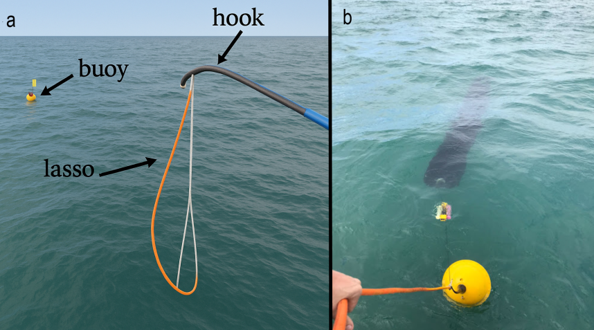
(4) Recovery will be facilitated using fast boats. For streakline type of deployment and longer experiments, it may be necessary to use auxiliary boats. It is good practice to begin recovery with the drifter farthest from shore and proceed toward those closer to the coast or port. Navigation can be highly assisted by the FindMeSpot web portal, including one sensor for the rescue boat, so that the navigation course can be easily determined (Figure A1). Spot Trace updates positions at 2.5-minute intervals, so in strong current environments, buoys might drift up substantially between updates. Flags and light to ensure visibility in rough seas, low-light, and foggy conditions. After visual contact, drifter recovery is best performed by two or three crew members at the bow, using a 4-m aluminum pole equipped with a hook and lasso. The lasso, made of polypropylene rope encased in a plastic hose, maintains an open shape for its effective use (Figure 8a). The pole facilitates the retrieval of fast-drifting buoys alongside the vessel, extending the operator’s reach on low-freeboard vessels. The lasso ensures secure capture, aiding vessel maneuvering and buoy towing, while minimizing the risk of drogue entanglement in the propeller or keel (Figure 8b). The drifter should be brought onboard starting with the buoy to prevent damage to the sensors, followed by the reel, cable, and drogue.

Figure 8
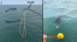
(a) Buoy approach and initial capture using a 4-m pole with a hook and lasso. (b) The drifter, secured by the lasso, is brought alongside the ship for retrieval, aided by the pole-mounted hook. Note the reel and extended drogue positioned away from the boat.

STUDY AREA DESCRIPTIONS

The study area encompasses distinct oceanographic settings in Brazil. The first is the coastal region between Ponta das Canas, north of the Florianópolis coast, and Arvoredo Island, in Santa Catarina State, southern Brazil, at 27°S, 48°W. The second is São Marcos Bay, in Maranhão State, northeastern Brazil, at 2°S, 44°W (Figure 2).

FLORIANÓPOLIS NORTHERN SHELF

Florianópolis shows a dynamic coastal environment shaped by winds, tides, and small local river discharges, which influence shelf circulation. Astronomical tides are mixed, predominantly semi-diurnal with small amplitudes, characterizing a microtidal regime (Truccolo et al., 2006). Previous hydrographic campaigns in this region recorded salinity ranging from 32 to 36.5 and temperatures between 14 and 28°C (Hille et al., 2008). The winter incursion of less saline, colder waters is attributed to the intrusion of Plata River plume waters (Möller Jr. et al., 2008, Pimenta and Kirwan, 2014).

Subtidal sea-level variability is significant in the meteorological band, driven primarily by-passing cyclones and anticyclones (Pimenta et al., 2004). On the eastern side of the island, previous waverider buoy rescue operations indicated mid-shelf currents aligned with the coastline (Pimenta et al., 2013). Earlier drifter deployments on the outer shelf also revealed coherent currents flowing along isobaths (Assireu et al., 2003; Souza and Robinson, 2004).

Near Arvoredo Island, ADCP campaigns indicated that currents are strongly correlated with wind and local sea level, the primary forcings at subtidal frequencies. Currents typically average 0.2 m s^-1, but during strong events, speeds exceeding 0.5 m s^-1 have been recorded (Dalbosco et al., 2020).

Two drifter deployments were conducted in October 2024 off northern Florianópolis Island (Figure 2a). The first, a cluster-type deployment off Ponta das Canas, investigated circulation and dispersion responses to southern winds. The second, a timeline-type deployment, investigated current structures and shelf-exchange processes with Florianópolis North Bay (Figure 2a).

SÃO MARCOS BAY

São Marcos is an estuary complex located in northeastern Brazil at 2.42°S, 44.30°W, situated at the transition between Amazonian and semiarid Brazilian climates (Lima et al., 2021; Santos et al., 2025). The estuary, commonly referred to as São Marcos Bay, features a well-developed ebb-dominated tidal channel oriented in a NE-SW direction (El-Robrini, 1992, 2006). Caranguejo Island further divides the bay into two channels in the inner part of the estuary. The bay’s length can reach 130 km, measured from Ponta da Raposa near the bay’s mouth up to the Mearim River. Our study area is situated in a 15 km wide channel between São Luís and Alcântara, a region characterized by depths between 10 and 50 m (Figure 2b).

The dominant tidal constituents are the principal lunar semidiurnal M2 and the principal solar semidiurnal S2, characterizing São Marcos as a hypersynchronous macrotidal estuary, where some areas experience tidal ranges exceeding 6 m (Azevedo et al., 2016; Czizeweski et al., 2020; Santos et al., 2025).

Tidal flow in the estuary’s main channels, derived from both models and observations, shows currents ranging from 1.5 to 2 m s^-1 (Czizeweski et al., 2020; Santos et al., 2025). River discharge to the bay is provided by two main contributions: the Mearim and Pindaré rivers (Figure 2). Mearim averages 708 m³ s^-1 but can reach 1240 m³ s^-1 during the wet season. Pindaré average discharge is 246 m³ s^-1 (Santos et al., 2025; SECID, 2014). Previous hydrographic campaigns conducted reveal surface salinity varying 20.5 to 30.5 (wet season) to 26.4 to 32.4 (dry season) between Caranguejo Island and Alcântara, also displaying a tendency for freshwaters to exit the estuary through the left of the channel (Lefèvre et al., 2017). Santos et al. (2025) based on hydrographic and current data classified São Marcos predominantly as a well-mixed estuary. During the neap tides and rainy season, the estuary might approach partially mixed conditions.

Tidal excursion length L is estimated to be between 21.4 and 28.5 km considering currents varying from 1.5 to 2 m s^-1 and semi-diurnal tidal frequency. Prevailing winds typically blow from the northeast. The region is dominated by the trade winds system, and sea breezes are an important component of coastal winds (Pimenta et al., 2023).

The experiment conducted in São Marcos Bay was designed to investigate the effects of tides and winds on its circulation. A cluster-type deployment was conducted in April 2025 near Porto do Itaqui, involving two coastal SVP drifters and one iSphere drifter. The iSphere buoy was undrogued but equipped with a Spot Trace device mounted inside its hull.

RESULTS

Field experiments were conducted on the Florianópolis northern shelf (SC) and in São Marcos Bay (MA) to validate the coastal drifter tracking system, achieving a 100% recovery rate. The drifters’ trajectories and velocities provided high-resolution data on the dynamics of these environments, highlighting the influence of tides, winds, and bathymetry on circulation.

FLORIANÓPOLIS NORTHERN SHELF

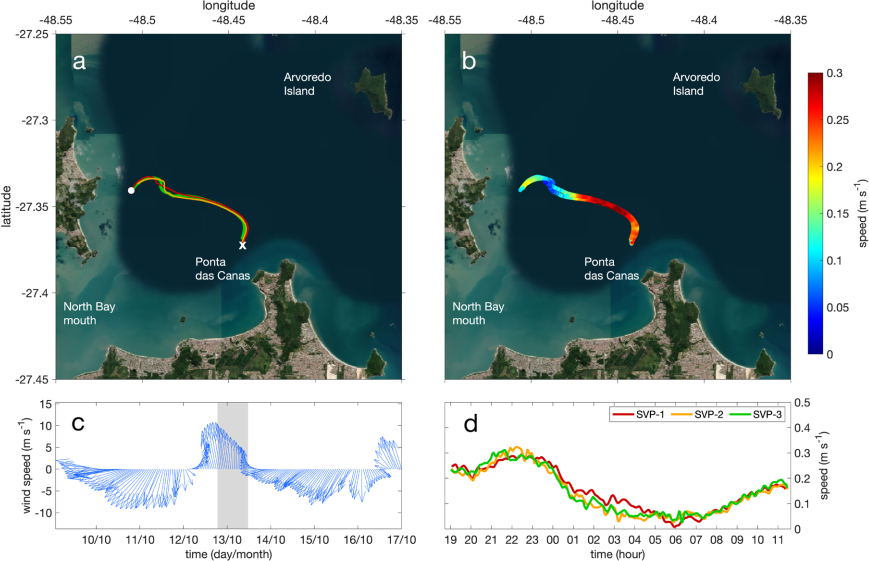
Two deployments followed by drifter recoveries were conducted in southern Brazil aboard the 60-foot sailboat ECO. The cluster-type deployment occurred at Ponta das Canas on October 12^th, 2024, at 19:00 UTC (16:00 local time), releasing three coastal SVP drifters. Figure 9a illustrates the drifter release point marked with an “X” and individual drifter tracks as colored lines. Drifters were launched at the onset of a relatively brief but strong southerly wind event with speeds of 5 to 10 m s^-1 (Figure 9c).

Figure 9
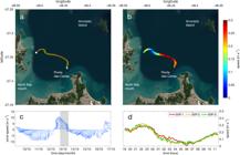
Deployment of three coastal SVP drifters in cluster mode at Ponta das Canas, southern Brazil, between October 12^th and 13^th, 2024. (a) Individual trajectories of SVP-1 (red), SVP-2 (orange), and SVP-3 (green), with the deployment location marked by an “X” and the recovery location by a white circle. (b) Drifter tracks, with the colorbar indicating speeds (m s^-1). (c) Time series of wind speeds from October 10^th to 17^th 2024, derived from ERA5 atmospheric reanalysis for a grid point located at 48.25^oW, 27.25^oS (Hersbach et al., 2020). A gray bar indicates the deployment period. (d) Time series of drifter speeds (m s^-1) from October 12^th, 19:00 to October 13^th, 11:00, 2024, with the x-axis representing UTC hours.

The drifters initially moved northward from Ponta das Canas at speeds up to 0.25 m s^-1 at the start of the experiment. As winds weakened, the drifters veered northwest. Figure 9b illustrates the evolution of drifter speeds along their tracks and Figure 9d shows time series of individual drifter speeds, with velocity components calculated from their positions using central differences. Drifter speeds peaked at 0.32 m s^-1 on October 12^th at 22:00 UTC, slowing to very low velocities by October 13^th at 05:00 UTC as they moved to the west.

With the onset of the flood tide and under easterly winds, the drifters moved toward the bay mouth with increasing speed past 08:00 UTC. The three trajectories remained closely aligned with minimal dispersion and were recovered on October 13^th around 11:00 UTC (Figure 9a).

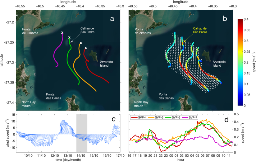
During the timeline deployment, increasing northeasterly winds prevailed (Figure 10). The operation involved four coastal SVP drifters, spaced 1.8 to 3.2 km apart, launched on October 13^th, 2024. Figure 10a illustrates the boat’s trajectory during the transect between Arvoredo Island and Ponta de Zimbros, with “X” symbols marking the drifters’ deployment locations. The transect was approximately 7.2 km long, began on October 13^th, 16:00 UTC and was completed in about 50 minutes.

Figure 10
Deployment of four coastal SVP drifters using the timeline method at Arvoredo, southern Brazil, between October 10^th and 14^th, 2024. (a) Individual trajectories of SVP-4 (red), SVP-5 (orange), SVP-6 (green), and SVP-7 (purple), with deployment locations marked by an “X”. (b) Drifter tracks, with the colorbar indicating speeds in m s^-1. White vectors indicate the interpolated near-surface velocity field derived from the drifter observations using an objective interpolation method. (c) Time series of wind speeds for 10 to 17 October 2024, derived from ERA5 atmospheric reanalysis for a grid point located at 48.25°W, 27.25°S (Hersbach et al., 2020). A gray bar indicates the deployment period. (d) Time series of drifter speeds (m s^-1) from October 13^th, 16:00 to October 14^th, 11:00, 2024, with the x-axis representing UTC hours.

All drifters initially followed a southward trajectory with velocities of 0.20 m s^-1, showing slight variations. Drifter SVP-4 (red line) maintained a southerly path, accelerated as it passed Arvoredo Island, then looped anticyclonically, likely induced by a vortex generated by the island’s wake.

SVP-5 (orange) followed a similar track, initially veering toward the bay mouth, but then making a wide anticyclonic turn to the southeast (Figure 10a). Both SVP-4 and SVP-5 drifters accelerated as they moved offshore (Figure 10b). Figure 10d illustrates that drifters’ speed increased from 0.1 m s^-1 on October 14^th at 00:00 UTC to 0.4 m s^-1 on October 14^th at 07:00 UTC, later decaying to 0.15 m s^-1 offshore. SVP-6 (green) also accelerated along its southeast trajectory. However, near the end of its path, the drifter turned southwest, diverging substantially from SVP-5’s track (orange) (Figure 10a).

Figure 10b displays the near-surface velocity field, with colors along the drifter tracks indicating speed. The white vector field was obtained by objectively interpolating the drifter-derived horizontal velocity components (u, v) following the approach of Bretherton et al. (1976). Given the non-stationary nature of the flow during the deployment period, this interpolated field should be interpreted with caution. Nevertheless, it provides a useful synoptic view of the circulation associated with the upwelling event. The vector field indicates southward currents west of Arvoredo Island that diverge near Ponta das Canas, with one branch entering the North Bay mouth and another merging with offshore shelf currents. This circulation pattern is consistent with previous modeling results for the region (Marta-Almeida et al., 2021).

SVP-7 (purple) initially moved southward, then shifted southwest before veering toward the bay mouth, where it was captured by a fishing boat (Figure 10a). The capture was detected during the fieldwork due to unrealistic speeds and trajectories (not shown). The equipment was recovered by pursuing the boat and contacting the local fisherman. The SVP-7 drifter, which was positioned closer to the coastline, exhibited lower speeds (Figure 10c). All drifters slowed down toward the end of the experiment. Apart from the winds shown in the ERA5 data (Figure 10c), which indicated a slight decay, local wind conditions were relatively mild during the offshore recoveries.

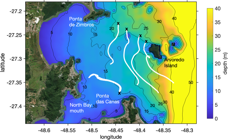
Figure 11 superimposes all drifter trajectories on bathymetry. During both the cluster-type and timeline deployments, the drifters remained in waters deeper than the limiting operational depth (12 m). The maximum depth reached was 40 m, recorded by drifter SVP-4 during the second deployment.

Figure 11
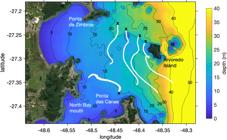
Drifter trajectories overlaid on a bathymetric map of the northern Florianópolis shelf, encompassing the region between Arvoredo Island, Ponta de Zimbros, and the mouth of the North Bay. SVP trajectories from the first and second deployments are shown as white tracks, with deployment positions indicated by black “X” symbols. Color shading and contour lines represent water depth (m).

SÃO MARCOS BAY

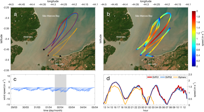
A cluster-type deployment was conducted in São Marcos Bay between April 1^st and 2^nd, 2025, aboard the catamaran Guará, using two coastal SVP drifters and one iSphere buoy instrumented with Spot Trace. Winds blew steadily from the northeast sector throughout the experiment, which spanned two ebb and two flood periods (Figure 12).

Figure 12
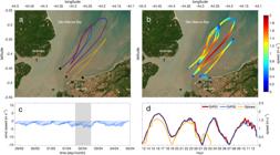
Deployment of two coastal SVP drifters and one undrogued iSphere drifter at São Marcos Bay, northeastern Brazil. (a) Individual trajectories of SVP-1 (red), SVP-2 (blue), and the undrogued iSphere (orange). The deployment location is marked with an “X” and recovery locations with black circles. (b) Drifter tracks, with the color bar indicating speeds in m s^-1. (c) Time series of wind speeds for 29 March to April 5^th 2025, derived from ERA5 atmospheric reanalysis for a grid point located at 44.25^oW, 2.5^oS (Hersbach et al., 2020). A gray bar indicates the deployment period. (d) Time series of drifter speeds (m s^-1) from April 1^st, 12:30 to April 2^nd, 13:00, 2025, with the x-axis representing UTC hours.

Drifters were released during syzygy on April 1^st at 13:00 UTC, near the 25 m isobath of a subchannel east of the main estuarine channel (Figure 12). The deployment coincided with the transition from flood to ebb tide. Consequently, all drifters initially followed short southwestward paths toward the estuary, before reversing to the northeast and extending offshore during the first ebb tide cycle (Figure 12a). SVP-1 (red) and SVP-2 (blue) reached approximately 27 km offshore before turning anticyclonically during the ebb-to-flood transition and circulating around a shallow shoal. Figure 13 shows this behavior more clearly by superimposing the drifter trajectories on the bathymetry. These drifters remained close and traveled back during the first flood cycle, reaching a region about 5 km north of the launch position (Figure 12a).

Although launched nearly simultaneously, the undrogued iSphere followed a markedly different trajectory. During ebb flow, it traveled east of the SVPs and its offshore excursion was notably shorter, approximately 20 km. The iSphere also showed a sharper turn during the ebb-to-flood transition (Figure 12a). During the flood, it traveled east of its initial ebb path and returned to a point about 2 km east of the deployment site, in significantly shallower waters (Figure 12a). At the onset of the next ebb cycle, the iSphere drifted eastward, induced by shore-parallel tidal currents but was ultimately carried by strong nighttime winds and waves, running aground at Praia do Calhau and recovered around April 2^nd at 03:00 UTC (Figure 12a).

During the second ebb cycle, SVP-1 and SVP-2 followed trajectories along the main channel, west of their first-cycle paths and the shallow bank located near 44.23°W, 2.35°S (Figure 13). The excursion length was shorter, reaching 17 km offshore, with an abrupt anticyclonic turn during the tidal shift. Notably, the drifters remained very close to each other throughout the experiment, and their return during the second flood cycle followed nearly identical routes. Both SVPs were recovered in the main channel on April 2^nd, 2025 at approximately 12:45 UTC (09:45 local time), at a depth of 40 m, at the location marked by a bullet (Figures 12a and 13).

Figure 13
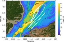
Drifter trajectories overlaid on a bathymetric map of São Marcos Bay, between Alcântara and São Luís. SVP and iSphere trajectories are shown as white tracks, with the deployment position indicated by a black “X” symbol. Color shading and contour lines represent water depth (m).

Peak velocities of 1.9 m s^-1 were recorded by the SVPs during the first ebb cycle (Figure 12b), while the iSphere reached a maximum of 1.6 m s^-1. The time series also indicate a decline in tidal current magnitudes following the drifters’ transition from a shallower subchannel to the main channel (Figure 12d, 13). This pattern is also evident in Figure 12b, which overlays drifter speeds along their trajectories. These changes in current speed are likely related to the complex bathymetry of the São Marcos estuary, where multiple banks and channels partition the tidal flow into distinct branches that interact with the shelf circulation, generating spatial variability in flow speeds, recirculation cells, and differences in the timing of ebb-flood reversals.

The iSphere trajectory likely results from the combined influence of tides, winds, and wave-induced circulation. Theory suggests that wide estuaries adjust to persistent onshore axial winds by generating downwind currents over shallow areas, while a barotropic upwind return flow prevails in the main channel (Sanay & Valle-Levinson, 2005; Wong, 1994). This mechanism may explain the reduced offshore extent of the iSphere trajectories relative to the SVPs. Wind drag is also a plausible factor influencing iSphere behavior. Pawlowicz et al. (2024) showed that the iSphere’s downwind slip is approximately 3-4% of the wind speed, which corresponds to 0.2-0.3 m s^-1 under 8 m s^-1 winds. This magnitude is comparable to the observed speed deficit relative to the SVPs (Figure 12d). Over the six-hour period, the iSphere’s offshore excursion was 7 km shorter, corresponding to an average speed of 0.32 m s^-1.

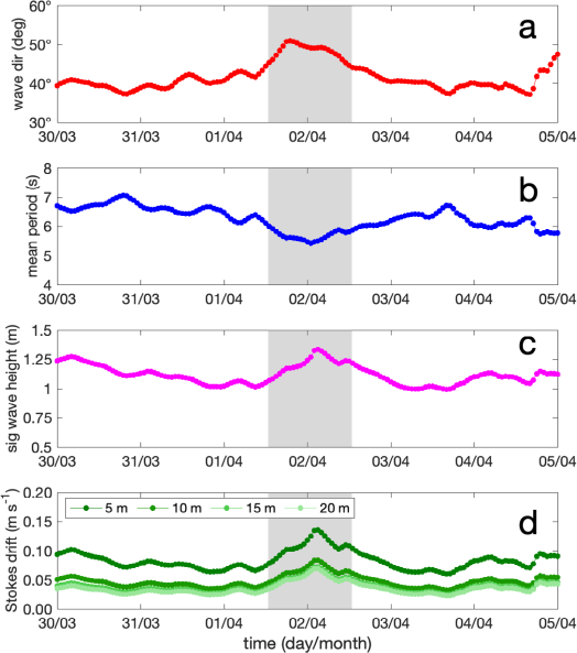
Regarding transverse excursion, the iSphere drifted approximately 2 km relative to the SVP trajectories over a six-hour period, corresponding to a mean cross-channel velocity of ~0.09 m s^-1. Wind drag may have contributed to this displacement, particularly if anticlockwise shifts in wind direction occurred relative to the estuarine axis; however, such short scale variability cannot be resolved by the ERA5 reanalysis. During the deployment, offshore wave conditions were characterized by periods between 4 and 6 s, a significant wave height of ~1 m, and a mean propagation direction varying between 44° and 51°N. A simplified estimate of the Stokes drift (Us) suggests surface velocities on the order of 0.05-0.1 m s^-1 (Figure A2).

According to theory, wave-induced drift increases in magnitude for shorter wave periods and shallower water depths. The combined effects of wave refraction and Stokes drift toward the eastern shore of São Marcos Bay could therefore provide a mechanism for the observed onshore displacement of the iSphere.

The influence of laterally sheared longitudinal tidal currents and Coriolis remains to be assessed (Chant, 2010). Sanay and Valle-Levinson (2005) demonstrated that transverse Ekman circulation may develop in estuaries in which h/d>1, with h representing the maximum depth and d the Ekman layer thickness. Despite the low latitude of São Marcos Bay (2.4° S), parameter analysis indicates h/d values ranging from 0.9 to 2, suggesting potential susceptibility to rotational effects¹. More extensive fieldwork combining wind, waves and current measurements would be necessary to clarify these dynamics. Finally, given the intense cargo ship traffic in São Marcos Bay, one SVP drifter was recovered with red paint marks on its buoy hull, most likely from a collision. This incident underscores the robustness of the coastal SVP drifter for field campaigns in busy port areas.

SPOT TRACE AND I-GOTU COMPARISONS

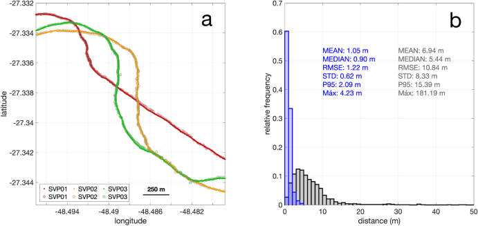
A direct comparison between the Spot Trace and i-gotU GNSS sensors was conducted during the Florianópolis deployments. Figure 14a illustrates a detailed track comparison, revealing strong agreement between the two sensors, although Spot Trace had some outliers. In contrast, the i-gotU’s raw data produced notably smoother tracks with minimal data loss, tracking an average of 11 satellites, ranging from 8 to 14. Data from the i-gotU installed on SVP-4 ceased operation during deployment.

Figure 14
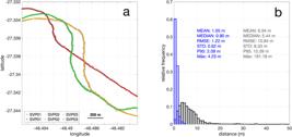
(a) Detailed view of the track records from the first deployment in Florianópolis. Large bullets denote Spot Trace positions for coastal drifters SVP-1 (red), SVP-2 (orange), and SVP-3 (green) updated every 2.5 minutes. Small dots of corresponding colors represent i-gotU positions recorded at one-second intervals for the same drifters. (b) Histogram of distances errors. The gray histogram depicts the differences between Spot Trace and i-gotU satellite track coordinates, derived from 1,306 coordinate pairs collected during two deployments. The blue histogram illustrates the distribution of errors for a static test where four i-gotU remained fixed in an open field location for two hours, collecting 28,803 coordinate points.

Sensors mounted on the same drifters were evaluated by calculating the distances between their recorded coordinates, using the WGS84 ellipsoid as the reference model. Vincenty’s formula was applied to compute the shortest path on the ellipsoid with high precision. Coordinate pairs (latitude and longitude) were synchronized to the nearest second, yielding 1,306 pairs for Florianópolis Deployments 1 and 2.

The gray histogram in Figure 14b shows the results. The mean distance error between the sensors was 6.94 m, with a median of 5.44 m. The root mean square error (RMSE) was 10.84 m, the standard deviation 8.33 m. The 95th percentile (P95) was 15.39 m, and the maximum outlier reached 181 m.

A complementary static test was subsequently conducted using i-gotU sensors to assess their precision. Four i-gotU units were mounted on a plastic sheet, fixed with zip ties, spaced 15 cm apart, and installed in an open grass field at Campeche Beach (48.4873°W, 27.6836°S), Florianópolis, on July 26^th, 2025. Since the i-gotU sensors may enter hibernation mode to conserve power, a small electric motor with a rotating pendulum was attached to the sheet to keep the sensors continuously vibrating and recording. The plastic sheet remained in a fixed position throughout the test. Distance errors were calculated based on the mean latitude and longitude recorded by each tracker.

A total of 28,803 positions were registered during a two-hour experiment with i-gotU sensors set to a one-second recording interval. Figure 14b shows the results as a blue histogram. The mean distance error between sensors was 1.05 m, with a median of 0.90 m. The RMSE was 1.22 m, the standard deviation was 0.62 m, the 95th percentile (P95) was 2.09 m, and the maximum error was 4.23 m. These metrics outperform those reported for the Spot Trace system, with static mean errors of 2.5 m (Pawlowicz et al., 2019) and 6 m (Lumpkin et al., 2017), and a P95 error of 10 m (Novelli et al., 2017).

Results indicate that i-gotU may significantly enhance drifter tracking accuracy, especially in areas with complex geography and flow patterns. In this study, Spot Trace latitude and longitude tracks were processed by removing outliers, interpolating to a one-minute interval, and applying a Gaussian smoothing filter.

CONCLUSIONS AND SUMMARY

This study presents the development and validation of a cost-effective real-time tracking system, alongside modifications to SVP drifters for coastal applications. Field tests were performed in two contrasting Brazilian coastal settings: the microtidal, wind-driven Florianópolis Northern Shelf and the macrotidal São Marcos Bay. The principal adaptations comprised a reel for adjustable drogue depth, a 3D-printed housing for electronic components, and integrated satellite communication systems (Spot Trace and Starlink) to ensure accurate tracking and reliable recovery.

Field experiments conducted in October 2024 off Florianópolis Island and in April 2025 in São Marcos Bay achieved full drifter recovery, demonstrating system robustness. At Florianópolis, both cluster and timeline deployments captured a rapid reversal of wind-driven circulation, with downwelling-favorable northwest flow under southerly winds and upwelling circulation under northeasterly winds. Divergent trajectories observed in the timeline deployment suggest modulation by local bathymetry and potentially by island-induced steering.

In São Marcos Bay, the cluster deployments revealed a predominantly tidal-driven circulation, with secondary modulation by wind and waves. The drogued SVP drifters tracked near-surface currents within the upper water column (3-9 m), governed primarily by barotropic tidal dynamics, following well-defined channel pathways and completing tidal excursions of 17-27 km.

In contrast, the undrogued iSphere, operating in the uppermost ~0.3 m, showed greater sensitivity to surface processes, indicating an enhanced response to wind and waves. The iSphere showed a shorter offshore excursion and a pronounced transverse (eastward) displacement. Although not fully resolved, its behavior is consistent with the combined effects of wind drag, wave-induced transport, and possibly wind-driven longitudinal and transverse estuarine circulation. More generally, these observations underscore that transport pathways can differ substantially depending on whether substances are confined to the surface layer or distributed throughout the water column.

The robustness of the drifters was also demonstrated: one coastal SVP drifter survived a collision with a cargo ship, while the iSphere was recovered from the beach. The real-time tracking system, powered by Starlink and the FindMeSpot portal, improved operational navigation, enabling rapid deployment adjustments and precise recovery. Optionally, drifters can be complemented with faster-response trackers, such as the i-gotU, providing supplementary data and balancing real-time tracking with higher-frequency data recording.

The financial viability of recoverable versus disposable drifters for coastal studies warrants consideration. Recoverable drifters consist of a hull (buoy and drogue) with an estimated cost of US$750, a Spot Trace device (US$80), an i-gotU sensor (US$100), an LED light (US$10) and a protective shelter (US$50) totaling about US$990 per unit². In contrast, disposable drifters include only the hull, protective shelter, and Spot Trace device, costing ~US$880 per unit.

In Brazil, boat rental rates are typically around US$1,000 per day. A deployment without recovery generally requires one day of vessel time, costing US$1000, whereas a deployment with recovery requires two days, costing US$2,000. Assuming a 100% recovery rate, the recoverable approach incurs only the vessel cost per operation, since drifters are reused. In contrast, the disposable approach incurs one day of vessel cost (US$1,000) plus the replacement of lost drifters (US$880 x N, where N is the number of drifters deployed). The break-even point occurs when the cost of the disposable approach equals that of the recoverable approach, yielding N~1.2. Thus, recovery becomes more cost-effective when deploying two or more drifters in a single operation, with savings increasing from US$760 for two drifters to US$7,800 for ten. For higher vessel costs, the break-even point shifts to N=3.4 for US$3,000/day and N=6 for US$5,000/day, making recovery less advantageous for few drifters’ deployment. Accounting for higher hull and drogue costs shifts the break-even point to even lower values of N. Beyond cost savings, the recoverable approach reduces environmental impact by preventing the permanent loss of equipment at sea and offers a scalable, low-cost solution for coastal studies.

The real-time tracking system based on Starlink and Spot Trace and i-gotU provides near-global coverage, enabling recovery across a wide range of environments, including rivers, lakes, fjords, estuaries, and coastal oceans. Satellite communication, however, depends on open-sky conditions and may be less effective in densely forested rivers and estuaries.

Compared with the classical SVP drifter configurations described in the literature, the cable reel system enables rapid adaptation for tracking near-surface currents between 3 and 9 m depth, extending the drifter’s operational range in coastal areas to approximately 12 m. High-visibility buoy painting, together with a signaling flag and LED light, significantly enhances recovery operations. Future improvements, such as manufacturing the cable reel from lightweight alloy materials, could reduce system weight and minimize or eliminate the need for auxiliary flotation. Moreover, a modular or sectional drogue design would enable further reduction of drogue length, enabling SVP operation in even shallower environments.

The robustness and adaptability of the SVP system make it suitable for repeated deployments across diverse aquatic environments to study transport and dispersion processes, while supporting research on marine ecosystems, port operations, and environmental monitoring.

FRMa $d=\sqrt{2A_z/\left|f\right|}$

DATA AVAILABILITY STATEMENT

Data are available upon reasonable request for academic, non-commercial research purposes.

SUPPLEMENTARY MATERIAL

The supplementary material is provided in the Appendix of this article.

ACKNOWLEDGMENTS

We express our gratitude to the Brazilian Navy and NOAA for the donation of SVP drifters. Alejandro Donnangelo Varela and the crews of the sailboat ECO and the catamaran Guará provided skilled and enthusiastic support. Luciano Cota skillfully constructed the reel systems used in the SVP drifters. Saulo Guths kindly provided space for painting the SVPs. Rumano L. Imbali helped with the Florianópolis operations. A.D. Kirwan and A. Valle-Levinson offered insightful and constructive feedback on the initial draft of this manuscript. D.P. Wang kindly provided the software used for constructing the vector fields. Bruna Alves and Rafael Quezada provided critical support in equipment handling and project management. We thank two anonymous reviewers for their constructive suggestions, which improved this manuscript, including the evaluation of wave-induced drift.

REFERENCES

• Andrade, M. M., Toldo Jr., E. E. & Nunes, J. C. 2016. Variabilidade das correntes na plataforma interna ao largo de Tramandaí, RS durante o verão de 2014. Pesquisas em Geociências, 43(3), 289-298. DOI: https://doi.org/10.22456/1807-9806.78231
  » https://doi.org/10.22456/1807-9806.78231
• Assireu, A. T., Pimenta, J. V., Saavedra, O. R., Camacho, R., El Robrini, M., Pimenta, F. M., Tiago Filho, G. L., & Cosme, D. S. 2026. Hydrokinetic energy assessment downstream of the hydroelectric Dam from GNSS-tracked drifters: a new approach. Renewable Energy, 258, 124905. DOI: https://doi.org/10.1016/j.renene.2025.124905
  » https://doi.org/10.1016/j.renene.2025.124905
• Assireu, A. T., Stevenson, M. R. & Stech, J. L. 2003. Surface circulation and kinetic energy in the SW Atlantic obtained by drifters. Continental Shelf Research, 23(2), 145-157. DOI: https://doi.org/10.1016/S0278-4343(02)00190-5
  » https://doi.org/10.1016/S0278-4343(02)00190-5
• Azevedo, J. W. J., Castro, A. C. L. & Santos, M. C. F. V. 2016. Siltation rate and main anthropic impacts on sedimentation of the São Luís tidal inlet - state of Maranhão, Brazil. Brazilian Journal of Oceanography, 64(1), 9-18. DOI: https://doi.org/10.1590/S1679-87592016092106401
  » https://doi.org/10.1590/S1679-87592016092106401
• Breivik, Ø. & Allen, A. A. 2008. An operational search and rescue model for the Norwegian Sea and the North Sea. Journal of Marine Systems, 69(1-2), 99-113. DOI: https://doi.org/10.1016/j.jmarsys.2007.02.010
  » https://doi.org/10.1016/j.jmarsys.2007.02.010
• Bretherton, F. P., Davis, R. E. & Fandry, C. B. 1976. A Technique for Objective Analysis and Design of Oceanographic Experiments Applied to MODE-73. Deep Sea Research, 23(7), 559-582. DOI: https://doi.org/10.1016/0011-7471(76)90001-2
  » https://doi.org/10.1016/0011-7471(76)90001-2
• Chant, R. J. 2010. Estuarine secondary circulation. In: Valle-Levinson, A. ed. Contemporary issues in estuarine physics (pp. 100-124). Cambridge: Cambridge University Press.
• Conomos, T. J., McCulloch, D. S., Peterson, D.H. & Carlson, P. R. 1972. Drift of surface and near-bottom waters of the San Francisco Bay system, California: March 1970 through April 1971. Miscellaneous Field Studies. DOI: https://doi.org/10.3133/mf333
  » https://doi.org/10.3133/mf333
• Csanady, G.T. 1982. Circulation in the coastal ocean. Dordrecht, D. Reidel Pub.
• Czizeweski, A., Pimenta, F.M. & Saavedra, O.R. 2020. Numerical modeling of Maranhão Gulf tidal circulation and power density distribution. Ocean Dynamics, 70, 667-682. DOI: https://doi.org/10.1007/s10236-020-01354-8
  » https://doi.org/10.1007/s10236-020-01354-8
• Dalbosco, A. L. P., Franco, D., Barletta, R. C. & Trevisan, A. B. 2020. Analysis of currents on the continental shelf off the Santa Catarina Island through measured data. Revista Brasileira de Recursos Hídricos, 25. DOI: https://doi.org/10.1590/2318-0331.252020180175
  » https://doi.org/10.1590/2318-0331.252020180175
• Davis, R. E. 1985. Drifter observations of coastal surface currents during CODE: the method and descriptive view. Journal of Geophysical Research, 90(C3), 4756-4772. DOI: https://doi.org/10.1029/JC090iC03p04756
  » https://doi.org/10.1029/JC090iC03p04756
• El-Robrini, M. 1992. Evolution rapide des fonds d’une zone estuaire: Le secteur d’Itaqui-Baie São Marcos, Maranhão (Brésil). In: Marie-Thérèse, M (Ed.). Evolution des littoraux de Guyane et de La zone caraïbe méridionale pendant le quaternaire (159-176). Paris: ORSTOM.
• El-Robrini, M., Marques J., V., Silva, M. A. M. A., El-Robrini, M. H., Feitosa, A. C., Tarouco, J. E. F., Santos, J. H. S. & Viana, J. R. 2006. Maranhão. In: Muehe, D. (Org.). Erosão e progradação do litoral brasileiro (87-130). Brasília: Ministério do Meio Ambiente.
• Geyer, W. R. 1989. Field Calibration of Mixed-Layer Drifters. Journal of Atmospheric and Oceanic Technology 6 (2): 333-42. https://doi.org/10.1175/1520-0426(1989)006<0333:FCOMLD>2.0.CO;2
  » https://doi.org/10.1175/1520-0426(1989)006<0333:FCOMLD>2.0.CO;2
• Griggs, G. B. 1974. Nearshore current patterns along the central California coast. Estuarine and Coastal Marine Science, 2(4), 395-405. DOI: https://doi.org/10.1016/0302-3524(74)90007-3
  » https://doi.org/10.1016/0302-3524(74)90007-3
• Guimarães, P. V., Ardhuin, F., Sutherland, P., Accensi, M., Hamon, M., Pérignon, Thomson, J., Benetazzo, A. & Ferrant, P. 2018. A surface kinematics buoy (SKIB) for wave-current interaction studies. Ocean Science, 14(6), 1449-1460. DOI: https://doi.org/10.5194/os-14-1449-2018
  » https://doi.org/10.5194/os-14-1449-2018
• Henderson, T., Vernes, K., Körtner, G. & Rajaratnam, R. 2018. Using GPS technology to understand spatial and temporal activity of kangaroos in a peri-urban environment. Animals, 8(6), 97. DOI: https://doi.org/10.3390/ani8060097
  » https://doi.org/10.3390/ani8060097
• Hersbach, H., Bell, B., Berrisford, P., Hirahara, S., Horányi, A., Muñoz-Sabater, J., Nicolas, J., Peubey, C., Radu, R., Schepers, D., Simmons, A., Soci, C., Abdalla, S., Abellan, X., Balsamo, G., Bechtold, P., Biavati, G., Bidlot, J., Bonavita, M., De Chiara, G., Dahlgren, P., Dee, D., Diamantakis, M., Dragani, R., Flemming, J., Forbes, R., Fuentes, M., Geer, A., Haimberger, L., Healy, S., Hogan, R. J., Hólm, E., Janisková, M., Keeley, S., Laloyaux, P., Lopez, P., Lupu, C., Radnoti, G., de Rosnay, P., Rozum, I., Vamborg, F., Villaume, S. & Thépaut, J.-N. 2020. The ERA5 global reanalysis. Quarterly Journal of the Royal Meteorological Society, 146(730), 1999-2049. DOI: https://doi.org/10.1002/qj.3803
  » https://doi.org/10.1002/qj.3803
• Hille, E., Schettini, F. A. C. & Ribeiro, M. R. 2008. Estrutura termohalina no litoral de Santa Catarina nos anos de 2005 e 2006. In: Braga, E. S. (Ed.). Oceanografia e mudanças Globais (pp. 371-381). São Paulo: Edusp.
• Ivichev, I., Hole, L. R., Karlin, L., Wettre, C. & Röhrs, J. 2012. Comparison of operational oil spill trajectory forecasts with surface drifter trajectories in the Barents Sea. Geology & Geosciences, 1(1), 1-8.
• Kakoulaki, G., MacDonald, D. G. & Cole, K. 2020. Calculating lateral plume spreading with surface lagrangian drifters. Limnology and Oceanography: Methods, 18(7), 346-361. DOI: https://doi.org/10.1002/lom3.10356
  » https://doi.org/10.1002/lom3.10356
• Kakoulaki, G., MacDonald, D. & Horner-Devine, A. R. 2014. The role of wind in the near field and midfield of a river plume. Geophysical Research Letters, 41(14), 5132-5138. DOI: https://doi.org/10.1002/2014GL060606
  » https://doi.org/10.1002/2014GL060606
• Kirwan, A.D., McNally, G., Chang, M. S., and Molinari, R. 1975. The Effect of Wind and Surface Currents on Drifters. Journal of Physical Oceanography 3(1): 361-68.
• Krauss, W. 1993. Ekman drift in homogeneous water. Journal of Geophysical Research, 98(C11), 20187-20209. DOI: https://doi.org/10.1029/93JC01898
  » https://doi.org/10.1029/93JC01898
• Kundu, P. K. & Cohen, I. M. 2004. Fluid Mechanics. 3rd ed. California, Elsevier Academic Press. 759 pp.
• Lefèvre, N., Silva, C. E. F., Noriega, C., Araujo, M. & Ibánhez, J. S. P. 2017. A source of CO2 to the atmosphere throughout the year in the Maranhense continental shelf (2°30’S, Brazil). Continental Shelf Research, 141, 38-50. DOI: https://doi.org/10.1016/j.csr.2017.05.004
  » https://doi.org/10.1016/j.csr.2017.05.004
• Lima, H. P., F. J. S. Dias, C. E. P. Teixeira, V. A. Godoi, A. R. Torres, and R. S. Araújo. 2021. Implications of Turbulence in a Macrotidal Estuary in Northeastern Brazil - The São Marcos Estuarine Complex. Regional Studies in Marine Science 47: 101947. https://doi.org/10.1016/j.rsma.2021.101947
  » https://doi.org/10.1016/j.rsma.2021.101947
• Lumpkin, R., Özgökmen, T. & Centurioni, L. 2017. Advances in the application of surface drifters. Annual Review of Marine Science, 9(1), 59-81. DOI: https://doi.org/10.1146/annurev-marine-010816-060641
  » https://doi.org/10.1146/annurev-marine-010816-060641
• Mariano, A. J., Ryan, E. H., Huntley, H. S., Laurindo, L. C., Coelho, E., Griffa, A., Özgökmen, T. M., Berta, M., Bogucki, D., Chen, S. S., Curcic, M., Drouin, K. L., Gough, M., Haus, B. K., Haza, A. C., Hogan, P., Iskandarani, M., Jacobs, G., Kirwan Jr., A. D., Laxague, N., Lipphardt Jr., B., Magaldi, M. G., Novelli, G., Reniers, A., Restrepo, J. M., Smith, C., Valle-Levinson, A. & Wei, M. 2016. Statistical properties of the surface velocity field in the northern Gulf of Mexico sampled by GLAD drifters. Journal of Geophysical Research: Oceans, 121(7), 5193-5216. DOI: https://doi.org/10.1002/2015JC011569
  » https://doi.org/10.1002/2015JC011569
• Marta-Almeida, M., Dalbosco, A., Franco, D. & Ruiz-Villarreal, M. 2021. Dynamics of river plumes in the South Brazilian Bight and South Brazil. Ocean Dynamics, 71(1), 59-80. DOI: https://doi.org/10.1007/s10236-020-01397-x
  » https://doi.org/10.1007/s10236-020-01397-x
• Méndez-Jiménez, A., Heyman, W. D. & Dimarco, S. F. 2015. Surface drifter movement indicates onshore egg transport from a reef fish spawning aggregation. Physical Geography, 36(4): 353-366. DOI: https://doi.org/10.1080/02723646.2015.1023243
  » https://doi.org/10.1080/02723646.2015.1023243
• Merlino, S., Locritani, M., Guarnieri, A., Delrosso, D., Bianucci, M. & Paterni, M. 2023. Marine litter tracking system: a case study with open-source technology and a citizen science-based approach. Sensors, 23(2), 935. DOI: https://doi.org/10.3390/s23020935
  » https://doi.org/10.3390/s23020935
• METOCEAN. 2017. iSPHERE. Nova Scotia, Dartmouth. Available from: Available from: https://metocean.com/wp-content/uploads/2017/09/iSPHERE-3.pdf Access date: 2025 Mar. 27.
  » https://metocean.com/wp-content/uploads/2017/09/iSPHERE-3.pdf
• Miranda, L. B., Castro, F. B. M. & Kjerfve, B. 2002. Princípios de oceanografia física de estuários. São Paulo, Edusp.
• Möller Jr., O. O., Piola, A. R., Freitas, A. C. & Campos, E. J. D. 2008. The effects of river discharge and seasonal winds on the shelf off southeastern South America. Continental Shelf Research, 28(13), 1607-1624. DOI: https://doi.org/10.1016/j.csr.2008.03.012
  » https://doi.org/10.1016/j.csr.2008.03.012
• Morey, S. L., Wienders, N., Dukhovskoy, D. S. & Bourassa, M. A. 2018. Measurement characteristics of near-surface currents from ultra-thin drifters, drogued drifters, and HF radar. Remote Sensing, 10(10), 1633. DOI: https://doi.org/10.3390/rs10101633
  » https://doi.org/10.3390/rs10101633
• Mullarney, J. C. & Henderson, S. M. 2013. A novel drifter designed for use with a mounted acoustic doppler current profiler in shallow environments. Limnology and Oceanography: Methods, 11(8), 438-449. DOI: https://doi.org/10.4319/lom.2013.11.438
  » https://doi.org/10.4319/lom.2013.11.438
• Niiler, P. P., Paduan, J. D., Sybrandy, A. L. & Sombardier, L. 1991. The WOCE/TOGA Lagrangian Surface Drifter. Oceans Conference Record (IEEE) 2: 839-43. https://doi.org/10.1109/oceans.1991.627966
  » https://doi.org/10.1109/oceans.1991.627966
• Niiler, P. P., Sybrandy, A. S., Bi, K., Poulain, P. M. & Bitterman, D. 1995. Measurements of the water-following capability of holey-sock and TRISTAR drifters. Deep-Sea Research Part I: Oceanographic Research Papers, 42(11-12), 1951-1964. DOI: https://doi.org/10.1016/0967-0637(95)00076-3
  » https://doi.org/10.1016/0967-0637(95)00076-3
• Novelli, G., Guigand, C. M., Cousin, C., Ryan, E. H., Laxague, N. J. M., Dai, H., Haus, B. K. & Özgökmen, T. M. 2017. A biodegradable surface drifter for ocean sampling on a massive scale. Journal of Atmospheric and Oceanic Technology, 34(11), 2509-2532. DOI: https://doi.org/10.1175/JTECH-D-17-0055.1
  » https://doi.org/10.1175/JTECH-D-17-0055.1
• Nunes, G. T., Efe, M. A., Barreto, C. T., Gaiotto, J. V., Silva, A. B., Vilela, F., Roy, A., Bertrand, S., Costa, P. G., Bianchini, A. & Bugoni, L. 2022. Ecological trap for seabirds due to the contamination caused by the Fundão dam collapse, Brazil. Science of the Total Environment, 807, 151486. DOI: https://doi.org/10.1016/j.scitotenv.2021.151486
  » https://doi.org/10.1016/j.scitotenv.2021.151486
• PACIFIC GYRE. 2023. Microstar drifter datasheet. Retrieved June 20, 2025, from Retrieved June 20, 2025, from https://www.pacificgyre.com/microstar-product
  » https://www.pacificgyre.com/microstar-product
• Pape III, E. H. & Garvine, R. W. 1982. The subtidal circulation in Delaware Bay and adjacent shelf waters. Journal of Geophysical Research, 87(C10), 7955-7970. DOI: https://doi.org/10.1029/JC087iC10p07955
  » https://doi.org/10.1029/JC087iC10p07955
• Pawlowicz, R., Hannah, C. & Rosenberger, A. 2019. Lagrangian observations of estuarine residence times, dispersion, and trapping in the Salish Sea. Estuarine, Coastal and Shelf Science, 225, 106246. DOI: https://doi.org/10.1016/j.ecss.2019.106246
  » https://doi.org/10.1016/j.ecss.2019.106246
• Pawlowicz, R., Chavanne, C. & Dumont, D. 2024. The water-following performance of various Lagrangian surface drifters measured in a dye release experiment. Journal of Atmospheric and Oceanic Technology, 41, 45-63. DOI: https://doi.org/10.1175/JTECH-D-23-0073.
  » https://doi.org/10.1175/JTECH-D-23-0073.
• Pazan, S. E. & Niiler, P. P. 2004. New global drifter data set available. Eos, Transactions American Geophysical Union, 85(2), 17. DOI: https://doi.org/10.1029/2004EO020007
  » https://doi.org/10.1029/2004EO020007
• Pimenta, F. M., Melo, E., Franco, D. & Zavialov, P. O. 2004. Assessment of Santa Catarina shelf currents through the analysis of indirect measurements. Journal of Coastal Research, (39), 651-55.
• Pimenta, F. M., Mendes, D. A. R., Souto, A., Melo, E., Vicentini Neto, F. L., Franco, D., Pereira, N. C., Castelão, G., Hammes, G., Barletta, R. & Romeu, M. A. R. 2013. Técnicas aplicadas no fundeio e manutenção de um ondógrafo direcional. Revista Brasileira de Recursos Hídricos, 18(2), 281-296. DOI: https://doi.org/10.21168/rbrh.v18n2.p281-296
  » https://doi.org/10.21168/rbrh.v18n2.p281-296
• Pimenta, F. M. & Kirwan Jr., A. D. 2014. The response of large outflows to wind forcing. Continental Shelf Research, 89, 24-37. DOI: https://doi.org/10.1016/j.csr.2013.11.006
  » https://doi.org/10.1016/j.csr.2013.11.006
• Pimenta, F. M., Saavedra, O. R., Oliveira, D. Q., Assireu, A. T., Torres Júnior, A. R., de Freitas, R. M., Albuquerque Neto, F. L., Lopes, D. C. P., Oliveira, C. B. M., de Lima, S. L., de Oliveira Neto, J. C. & Veras, R. B. S. 2023. Characterization of wind resources of the east coast of Maranhão, Brazil. Energies, 16(14), 5555. DOI: https://doi.org/10.3390/en16145555
  » https://doi.org/10.3390/en16145555
• Poulain, P.-M. & Gerin, R. 2019. Assessment of the water-following capabilities of CODE drifters based on direct relative flow measurements. Journal of Atmospheric and Oceanic Technology, 36(4), 621-633. DOI: https://doi.org/10.1175/JTECH-D-18-0097.1
  » https://doi.org/10.1175/JTECH-D-18-0097.1
• Richardson, P. L. 2009. Drifters and floats. Encyclopedia of Ocean Sciences, 171-178.
• Sanay, R. & Valle-Levinson, A. 2005. Wind-induced circulation in semienclosed homogeneous, rotating basins. Journal of Physical Oceanography, 35(12), 2520-2531. DOI: https://doi.org/10.1175/JPO2831.1
  » https://doi.org/10.1175/JPO2831.1
• Santos, V. H. M., Dias, F. J. S., Torres Júnior, A. R. & Sousa-Filho, P. W. M. 2025. Estuarine circulation in a tropical macrotidal estuary on the Amazon coast: relating thermohaline structure and suspended particulate matter concentration. Estuaries and Coasts. DOI: https://doi.org/10.1007/s12237-025-01562-9
  » https://doi.org/10.1007/s12237-025-01562-9
• SECID. 2014. Resumo do diagnóstico do plano diretor da bacia hidrografica do Mearim - MA. Vol. I. São Luís, Editora.
• Schmidt, W. E., Woodward, B. T., Millikan, K. S., Guza, R. T., Raubenheimer, B. & Elgar, S. 2003. A GPS-tracked surf zone drifter. Journal of Atmospheric and Oceanic Technology, 20(7), 1069-1075. DOI: https://doi.org/10.1175/1460.1
  » https://doi.org/10.1175/1460.1
• Siji, P. & Pattiaratchi, C. 2025. Surface current observations in the southeastern tropical Indian Ocean using drifters. Journal of Marine Science and Engineering, 13(4), 717. DOI: https://doi.org/10.3390/jmse13040717
  » https://doi.org/10.3390/jmse13040717
• Souza, R. B. & Robinson, I. S. 2004. Lagrangian and satellite observations of the Brazilian Coastal Current. Continental Shelf Research, 24(2), 241-262. DOI: https://doi.org/10.1016/j.csr.2003.10.001
  » https://doi.org/10.1016/j.csr.2003.10.001
• Subbaraya, S., Breitenmoser, A., Molchanov, A., Müller, J., Oberg, C., Caron, D. A. & Sukhatme, G. S. 2016. Circling the seas: Design of Lagrangian drifters for ocean monitoring. IEEE Robotics and Automation Magazine, 23(4), 42-53.
• Terrill, E., Thomas, J., Footer, A., Rosenfeld, L., Largier, J. & Williams, D. 2014. 2012 Orange County Sanitation District (OCSD) outfall diversion - Summary Report. San Diego, Scripps Institution of Oceanography. 189 pp.
• Truccolo, E C, Franco, D. & Schettini, F. 2006. The low frequency sea level oscillations in the northern coast of Santa Catarina, Brazil. Journal of Coastal Research, 39: 547-552.
• Tseng, R.-S. 2002. On the dispersion and diffusion near estuaries and around islands. Estuarine, Coastal and Shelf Science, 54(1), 89-100. DOI: https://doi.org/10.1006/ecss.2001.0830
  » https://doi.org/10.1006/ecss.2001.0830
• van Sebille, E., Zettler, E., Wienders, N., Amaral-Zettler, L., Elipot, S. & Lumpkin, R. 2021. Dispersion of surface drifters in the Tropical Atlantic. Frontiers in Marine Science, 7, 607426. DOI: https://doi.org/10.3389/fmars.2020.607426
  » https://doi.org/10.3389/fmars.2020.607426
• van der Mheen, M., Pattiaratchi, C., Cosoli, S. & Wandres, M. 2020. Depth-Dependent Correction for Wind-Driven Drift Current in Particle Tracking Applications. Frontiers in Marine Science, 7, 305. DOI: https://doi.org/10.3389/fmars.2020.00305
  » https://doi.org/10.3389/fmars.2020.00305
• Wong, K. C. 1994. On the nature of transverse variability in a coastal plain estuary. Journal of Geophysical Research, 99(C7), 14209-14222. DOI: https://doi.org/10.1029/94JC00861
  » https://doi.org/10.1029/94JC00861
• Woodbury, S K. 2017. Tracking oil spills around the world. McLean, MetOcean Telematics. Available from: Available from: https://metocean.com/wp-content/uploads/2017/09/MetOcean-iSPHERE-Oil-Spill-Tracking-Buoy-2020.pdf Access date: 2025 Apr. 27.
  » https://metocean.com/wp-content/uploads/2017/09/MetOcean-iSPHERE-Oil-Spill-Tracking-Buoy-2020.pdf

• 1
  Here the Ekman depth is defined as FRMa, in which Az is the vertical eddy viscosity (m² s^-1) and f as the Coriolis parameter. Considering h=50 m and Az values of 0.01 to 0.002 m² s^-1 the ratio h/d in São Marcos Bay ranges from 0.9 to 2.
• 2
  The Spot Trace price in Brazil is approximately R$800, with door-to-door delivery. The LED light costs R$60, the shelter fabrication (3D printing) R$300, and the imported i-gotU device incurs an additional importation cost of approximately 20%.
• AI USE STATEMENT
  Artificial intelligence tools (ChatGPT, OpenAI) were used exclusively to refine the English language of this manuscript. The content was carefully reviewed by the authors to ensure consistency and correctness. Authors are fully responsible for the final version of the manuscript.
• FUNDING
  This research was supported by the National Institute for Fluvial and Oceanic Energies of Brazil (INCT/INEOF, CNPq Process 465672/2014-0) and the National Ocean Observation and Monitoring Network (CNPq GOOS/Brasil, Process 409666/2022-0).

APPENDIX

Figure A1
Example of the FindMeSpot web portal accessed via Starlink during field operations, showing the tracks of the vessel and four coastal SVP drifters.

Figure A2
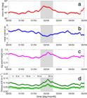
Wave conditions derived from ERA5 reanalysis for the period March 30^th to April 5^th at a grid point located at 44°W, 2°S (Hersbach et al., 2020). Panels show (a) mean wave direction (°N), (b) mean wave period (s), (c) significant wave height, Hs (m), and (d) surface Stokes drift, Us (m s^-1), estimated for water depths of h=5, 10, 15, and 20 m. Stokes drift was computed as Us=(Hs/2)² ωk [cosh(2kh)/(2 sinh²(kh))], where ω=2π/T and k was obtained from the full dispersion relation (Kundu and Cohen, 2004).

Edited by

• Associate Editor:
  Mauro Cirano

Publication Dates

• Publication in this collection
  31 July 2026
• Date of issue
  2026

History

• Received
  14 Sept 2025
• Accepted
  10 Mar 2026