Optimizing Laser Welding of Dissimilar Aerospace Materials: A Multiphysical Modeling Approach for Heat Flux and Residual Stresses in AA6013/Ti-6Al-4V Joints

Abstract

Optimizing laser welding of dissimilar materials is critical for aerospace applications, where high-performance joints are required under stringent weight and reliability constraints. This study presents a multiphysics modeling framework for predicting heat flux and residual stress development in laser-welded AA6013/Ti-6Al-4V dissimilar joints. A finite element model was implemented in COMSOL Multiphysics to simulate transient heat transfer, thermal gradients, and thermo-mechanical stress evolution, and was validated against experimentally measured thermal cycles, yielding deviations of 2.5–6%. The results demonstrate that heat input (HI) and beam offset strongly govern the temperature field, residual-stress distribution, and intermetallic-compound (IMC) formation at the Al/Ti interface. For condition T7 (HI = 9.6 J/mm; offset = 0.3 mm), the model predicted a peak temperature of 5950 K in the high-energy interaction region. A comparison between conditions T6 and T9 showed that, under identical beam intensity, reducing the welding speed increased the energy absorbed by the titanium side, with a 22% reduction in heat dissipated by conduction relative to T6. Residual stresses decreased with distance from the laser path; for a fixed offset, increasing HI increased compressive residual stress, reaching a maximum of 26 MPa (≈10% of the AA6013 yield strength) at HI = 24 J/mm and remaining nearly constant thereafter. In addition, higher cooling rates reduced IMC thickness from approximately 7 µm to 3 µm, indicating improved metallurgical conditions. Overall, the validated model provides a predictive tool for selecting process parameters to minimize residual stresses and control IMC growth, supporting the development of aerospace-grade AA6013/Ti-6Al-4V dissimilar laser welds.

Keywords:
Laser welding; Dissimilar joints; Multiphysical modeling; Residual stresses; Intermetallic compounds; AA6013; Ti-6Al-4V

1. Introduction

In aerospace structures, dissimilar aluminum–titanium joints are attractive for enabling lightweight hybrid designs that combine the high specific strength, corrosion resistance, and temperature capability of titanium with the low density and formability of aluminum alloys. Such joints are relevant for transition connections and local reinforcements in airframes where titanium fittings or frames interface with aluminum skins, stringers, or stiffened panels, and where galvanic/corrosion and thermal constraints motivate the use of titanium locally while retaining aluminum in less demanding regions. Laser beam welding is particularly appealing for these applications due to its high energy density, low overall heat input, and potential for controlled interfacial reactions compared with conventional fusion joining routes. Prior investigations on Al–Ti laser welding—including dissimilar AA6013/Ti6Al4V joints for aerospace-oriented solutions—highlight that process-window control is essential to limit intermetallic compound (IMC) growth and to obtain adequate joint integrity¹.

Laser beam welding (LBW) is widely adopted in high-value manufacturing sectors such as aerospace, automotive, and medical devices due to its high energy density, small heat-affected zone (HAZ), and high processing speed. In aerospace structures, dissimilar aluminum–titanium joints are particularly attractive for lightweight hybrid designs that combine the low density and good formability of aluminum alloys with the high specific strength and corrosion resistance of titanium alloys. Typical applications include transition joints and local reinforcements where titanium components (e.g., fittings, frames, or inserts) must be integrated with aluminum skins, stringers, or stiffened panels. However, the reliability of Al/Ti dissimilar welds remains highly sensitive to process parameters, motivating predictive tools that support parameter selection and quality optimization².

Numerical simulation has therefore become increasingly relevant for LBW process development, because it can reduce trial-and-error experimentation, identify defect-prone process windows, and improve joint quality while lowering manufacturing cost. In addition, computational models can support industrial decision-making by accelerating parameter optimization and improving production-line robustness. Mathematical and numerical approaches have been developed to estimate residual stresses and distortions generated during welding, and the finite element method (FEM) is one of the most widely used techniques to predict thermal fields and the resulting metallurgical and mechanical consequences in welded joints. The earliest analytical treatment of welding heat sources is commonly attributed to Rosenthal, who provided solutions for moving heat sources under simplified assumptions³.

Since then, numerous heat-source models have been proposed for arc welding, high-energy beam welding (electron beam and laser), and even solid-state joining processes, using both two-dimensional (2D) and three-dimensional (3D) approaches. More recently, “thermal simulation in four dimensions (TS4D)”—three spatial dimensions plus time—has been applied to handle multiple heat sources, surface sinks, dissimilar materials, and diverse surface cooling mechanisms, enabling both steady-state and transient predictions⁴.

A comprehensive literature review covering approximately 230 FEM-based welding studies (including ~150 focused on laser welding) reported that most thermal solutions are ultimately derived from the heat-conduction equation under appropriate boundary conditions⁵. Furthermore, Multiphysics simulation provides better understanding and mastery of processes. The biggest challenge in laser welding simulation is the interaction among the various phenomena involved in the process, such as photon-electron interactions, part distortion, and keyhole behavior.Despite advances in computational performance, a simulation approach encompassing everything from light propagation to structural distortion is currently not feasible, as it would require substantial computational power. Research about this type of simulation shows that numerical codes developed are restricted to simulating certain phenomena separately and then relate to the results obtained. Usually, the first step is the interaction of the laser with the material, investigating the heat transfer and the flow of the molten material.

Despite significant advancements, there remains a need for comprehensive multiphysical models that can accurately simulate the complex interactions between heat flux, residual stresses, and material behavior in laser welding of dissimilar joints. Existing models often lack the capability to integrate multiple physical phenomena and their impacts on joint integrity comprehensively⁶. Additionally, validation of these models with experimental data is essential to ensure their accuracy and reliability.

By the time-dependent heat function, it is possible to solve the problems related to the metallurgical behavior and obtain the mechanical properties of the welded joint. A common approach in the literature is that simulations of heat transfer and fluid flow are coupled with a frontal tracking method (or free surface) and a multiple reflection consideration⁷,⁸. The limitation to calculate all phenomena involved reduces the boundary conditions of the study. For example: the transfer of energy from the laser to the workpiece is usually approximated by the absorption coefficient of the material.

Pang, Chen, and Wang have found that the simulation using the Eulerian method can calculate the instability of the keyhole in addition to predicting pores formation⁹,¹⁰. In other studies, the best results were identified for the simulations that considered the various reflections of the laser, the heat transfers with the molten metal, the gas flow, the displacement of the free surface interface liquid/gas and the careful calculation of the recoil pressure¹¹. On the other hand, Level Set and VoF methods have presented limitations to calculate the size and type of mesh adopted to represent the spatter that can occur in laser welding. The front tracking method, with Lagrangian treatment of the interface¹⁰ or the Fluid Moment (Eulerian) method¹² are promising alternatives to reduce the numerical size of the problem and optimize the simulation results.

Laser welding of dissimilar lightweight alloys—particularly aluminum and titanium—remains challenging due to the pronounced mismatch in thermophysical properties, which promotes highly non-uniform heating/cooling and restricts stable interfacial wetting/spreading, thereby compromising joining quality. Moreover, dissimilar couples are prone to forming brittle intermetallic compounds (IMCs) at the interface, which can dominate failure behavior if their thickness and continuity are not controlled. Recent studies on dissimilar laser-based joining emphasize that these limitations originate from property mismatch and IMC formation, and further highlight that interface engineering approaches (e.g., transition layers or tailored interfacial conditions) can mitigate mismatch effects and enhance bonding reliability. In Al/Ti laser welding, these issues motivate the need for process-parameter optimization (e.g., heat input and offset) and predictive modeling capable of linking thermal fields to residual-stress evolution and IMC growth¹³.

In this context, the work aimed to develop a multiphysical modeling of heat flux and residual stresses generated by the laser to optimize the laser welding process of the dissimilar joint between AA6013 and the titanium alloy Ti-6Al-4V (AA6013/Ti-6Al-4V), both of which are used in the aerospace industry.

The study simulated and identified the influence of heat input (HI) and offset (the distance from the beam incidence to the interface between the two sheets). The modeling and simulation were validated by experimental data. In other words, the models developed can be used to estimate the joint regions, the formation of intermetallic compounds (IMCs), and the mechanical properties of the dissimilar joint (AA6013/Ti-6Al-4V) welded by laser beam.

2. Materials and Methods

As base metals for the experimental study, two dissimilar sheets were employed: an AA6013-T4 aluminum alloy and a Ti-6Al-4V (Grade 5) titanium alloy. Both sheets measured 100 mm × 50 mm × 1.6 mm and were cut to size using a guillotine shear. The T4 temper of the AA6013 sheet indicates that the alloy was solution heat-treated, rapidly quenched, and naturally aged.

Both the titanium and aluminum sheets were used in the as-received condition. The Ti-6Al-4V sheet was manufactured by hot rolling and subsequently annealed in accordance with ASTM B265¹⁴, whereas the AA6013-T4 sheet complied with the supplier’s temper specification described above. For both materials, the rolling direction was preserved during specimen preparation. The chemical compositions of the alloys are listed in Table 1¹⁵, and their mechanical properties are summarized in Table 2¹⁶-¹⁸.

Table 1
Chemical composition of base metal, wt.%.

	Al	C	Fe	Ti	V	Mn	Si	Cu	Mg	Zn
Ti-6Al-4V*	5.72	0.06	0.37	Base	4.10	-	-	-	-	-
AA 601315	Base	-	0.50	0.10	-	0.80	1.00	1.00	1.20	0.25

• ^*
  According to the manufacturer

Table 2
Mechanical properties of the base metals.

Base metal	Tensile strength (MPa)	Yield limit (MPa)	Modulus of elasticity (GPa)	Elongation (%)
AA601316,17	350	230	53	28
Ti-6Al-4V1,18	895	830	114	10

2.1. Experimental setup

The welding experiments were performed using an IPG YLR-2000 fiber-laser welding system installed at the Multiuser Laboratory for the Development of Laser and Optics Applications (DEDALO), Photonics Division (EFO), Institute for Advanced Studies (IEAv). The system is a continuous-wave (CW) ytterbium-doped fiber laser with a rated average power of 2 kW. It employs a 5 m delivery fiber with a 50 µm core, a beam parameter product (BPP) of 6.3 mm·mrad, and operates at a wavelength of 1.07 µm. The laser beam exhibited a near-Gaussian (TEM₀₀-like) intensity distribution, with a beam quality factor of M² ≈ 9 and a nominal beam diameter of 0.1 mm at the workpiece.

During welding, argon was supplied as the shielding gas for the molten pool at a flow rate of 18 L/min, while nitrogen was used to protect the optical system. The welding conditions were identical to those described in¹. The laser beam was directed toward the Ti-6Al-4V side (Figure 1), and the offset values are listed in Table 3.

Figure 1
Schematic drawing of the laser welding processing.

Table 3
Welding conditions and offset values.

Sample	Power (kW)	Offset (mm)	Welding speed (mm/s)	Heat input (J/mm)
T1	1.20	0.5	33.3	14.4
T2	1.00	0.5	33.3	12.0
T5	1.20	0.3	33.3	14.4
T6	1.00	0.3	33.3	12.0
T7	1.20	0.3	50.0	9.6
T8	1.00	0.3	50.0	8.0
T9	1.00	0.5	16.6	24.0

2.2. Description of modeling and simulation

The COMSOL Multiphysics software was chosen for its advanced capabilities in modeling the complex interactions involved in laser welding, particularly for dissimilar material joints like AA6013 and Ti-6Al-4V. Its multi-physics environment enables the coupling of heat transfer, structural mechanics, and material-specific properties, which are crucial for accurately predicting heat flux and residual stress distributions in such joints¹⁹.

The software's ability to simulate non-linear material behaviors and handle distinct thermal and mechanical properties of aluminum alloys and titanium alloys ensures realistic and reliable results. Moreover, its robust meshing algorithms and parametric study tools allow for detailed analysis of the effects of laser parameters, providing insights into optimizing the welding process. The integrated post-processing features deliver high-resolution visualizations, facilitating clear representation and interpretation of results, which are indispensable for correlating with experimental validations.

A three-dimensional model was developed to simulate the energy input and the residual stresses generated during the laser welding process of the dissimilar AA6013/Ti-6Al-4V joint. To make the simulation as close as possible to the experimental behavior and to reduce computational time, the following assumptions were made:

• The metallic alloys involved are homogeneous and isotropic materials.

• The laser beam exhibits a Gaussian profile with TEM00 mode²⁰.

• Heat conduction through the sheet is greater than any heat exchange with the environment by convection or radiation²¹.

• The temperature inside the keyhole is uniform, $T_{keyhole}=T_{vap}$.

• The weld face and root are nearly flat.

• Heat transfer equations for solid-state phenomena were applied.

• The keyhole exhibits stable behavior with a conical geometry²².

COMSOL Multiphysics software enables the addition of new physical properties or the creation of custom materials in its database. The thermophysical properties of the base metals, including specific heat, thermal conductivity, emissivity, and absorption coefficients, were obtained from validated datasets and correlations presented in Ribeiro²³. These data, originally developed and verified through experimental procedures in his doctoral research, were implemented in the present model to ensure realistic thermal behavior and accuracy in the simulation of heat flow and residual stress distribution during laser welding.

2.3. Heat flow modeling

The physical phenomena considered in developing the heat flow model included heat transfer, molten metal flow, mass transfer in terms of diffusion between chemical species, and solid mechanics for evaluating residual stresses. The mathematical treatment, representing the physical characteristics, corresponds to the solution of partial differential equations with appropriate boundary conditions. The interaction between the physical phenomena and the solution of the equations involved in the developed model was implemented using COMSOL Multiphysics™ Version 5.6.

The modeling of the heat input was determined by the nonlinear conservation of energy, being a function of the position and time according to Equation 1.

$\begin{array}{c}\rho \left(T\right)c_p^{eq}\left(T\right)\left(\frac{\partial T}{\partial t}\right)+\\ \rho \left(T\right)c_p\left(T\right)\overrightarrow{u}\overrightarrow{\nabla }T=\overrightarrow{\nabla }.\left(k\overrightarrow{\nabla }T\right)+q_L\end{array}$ (1)

In this equation $c_p^{eq}$ refers to the equivalent specific heat used to account for the latent heat of fusion ($L_f$, see Equation 2²⁴), $c_p$ is the specific heat, $\overrightarrow{u}$ is the velocity vector, $k$ is the thermal conductivity and $q_L$ is the effective energy for processing, resulting from the energy density deposited on the sheet by the laser beam.

$c_p^{eq}\left(T\right)=c_p^0\left(T\right)+L_f\frac{ex{p}^{\left(\frac{-{\left(T-T_{fus}\right)}^2}{\Delta T^2}\right)}}{\sqrt{\pi \Delta T^2}}$ (2)

$c_p^{eq}\left(T\right)$ can also be written as Equation 3:

$c_p^{eq}=c_p+D_m.L_f+D_v{L}_v$ (3)

$D_m$ and $D_v$ refer to the normalized Gaussian function for the melting and evaporation temperatures, respectively. Thus, the equivalent specific heat method is employed to describe the mushy phase (Equation 4).

$D_i=\frac{e^{\frac{-{\left(T-T_i\right)}^2}{\Delta T}}}{\sqrt{\pi \Delta T^2}}$ (4)

Where $\Delta T$ is a 50 K attenuation range

Assuming the laser energy distribution, where $q_L$ is represented by a Gaussian heat source applied to the top of the butt joint, and considering a continuous moving beam, we have the Equation 5:

$q_L=\frac{P_{L}A}{\pi r_0^2}{e}^{\left(\frac{-{\left(x+V_w.t\right)}^2+y^2}{r_0^2}\right)}$ (5)

Where $V_w$ is the welding speed, $r_0$ is the beam radius, and $P_L$ is the beam power (intensity). The laser radiation absorption coefficient for each material ($A$) is given by Equation 6:

$A=A_{solid}+\left(A_{líquido}{A}_{solid}\right).flc2h\left(T-T_{m,}\Delta T\right)$ (6)

$flc2h$ corresponds to the Heaviside function centered on the melting temperature ($T_m$) transitioning from 1 to 0 over the transition range $\Delta T$. This function accounts for changes in absorption values during melting, approximating the solid-liquid transition as a smooth step with a continuous second derivative, thereby reducing the computational load associated with logical true-step conditions²⁵,²⁶. In the Equation 7, such absorption in the liquid phase considers photon trapping in the keyhole due to critical penetration ($z_c$) defined as:

$A_{líquido}=A_{surf}+\left(A_{kh}-A_{surf}\right).flc2h\left(z-z_c,\Delta z\right)$ (7)

The other heat transfer mechanisms (convection and radiation) were also considered. Heat loss from the surface of the sheets was described by Equation 8.

$Q=h\left(T_s-T_0\right)+\sigma \epsilon \left(T_s{}^4-T_0{}^4\right)$ (8)

Where $Q$ represents the total heat loss due to convection and radiation, $T_s$ is the surface temperature, and $T_0$ is the ambient temperature. Note that the convective heat transfer coefficient is denoted b $h$. Similary, $\epsilon$ and $\sigma$ correspond to the material emissivity and the Stefan-Boltzmann constant, respectively.

The time step adopted in solving the computational model was 0.01 s. The total analysis time was associated with the derivative of the heat source position for each welding condition.

The heat source displacement is a function of time according to the Neumann boundary condition, relating Equation 5, the Gaussian heat source, and the radial coordinate ($r$):

$r=\sqrt{{\left(x-vt\right)}^2+y^2}$ (9)

2.4. Mesh study used in the modeling

Figure 2 illustrates the geometry, including the size and distribution of the mesh elements used in the model across the three domains, where a free tetrahedral mesh was applied. The largest element size was 2 mm, and the smallest was 0.02 mm for the titanium and aluminum sheet domains. However, for the domain representing the laser path, a more refined mesh was used, with the largest element size of 0.1 mm and the smallest of 0.0015 mm.

Figure 2
Mesh size and distribution of finite elements used for heat flow simulation.

The objective of using varying element sizes and distributions across the domains was to reduce processing time. The generated mesh presented 52,779 degrees of freedom (DOF), where the number of degrees of freedom corresponds to the product of the number of nodes and the number of dependent variables.

Similarly, a mesh refinement study was conducted to relate the physical phenomena of heat transfer and solid mechanics adopted in the modeling of residual stresses. Swept triangular elements with sizes smaller than the laser beam radius were used to construct the mesh for the laser path domain²⁷.

For domains 1 and 3, the mesh characteristics were selected based on a refinement study in which four types of meshes (TM) were compared to assess their impact on von Mises stress analysis results.

Table 4 summarizes the characteristics of the mesh types. The processing time for TM4 was approximately seven times longer than that for TM3, despite having a similar average element quality. Figure 3 demonstrates that the von Mises stress values for these two conditions are comparable. Consequently, the "Type 3" mesh configuration was adopted in the model.

Table 4
Mesh refinement study.

Characteristics	Mesh Type 1	Mesh Type 2	Mesh Type 3	Mesh Type 4
Geometry	Tetrahedral	Tetrahedral	Tetrahedral	Tetrahedral
Number of Elements	1456	3023	4346	10846
Average Element Quality	0.50	0.58	0.63	0.65
Mesh Volume	3040 mm2	3040 mm2	3040 mm2	3040 mm2
Total Processing Time	2 h 30 min 56 s	2 h 40 min	2 h 50 min	13 9 min

Figure 3
Von Mises Stress Values Associated with Different Meshes.

2.5. Residual stress modeling

Residual stress modeling was performed using data obtained from the heat flow analysis. The total strain was decomposed into three components, as described in Equation 10²⁸.

${\epsilon }_T={\epsilon }^e+{\epsilon }^p+{\epsilon }^{ts}$ (10)

Where: ${\epsilon }^e$ - elastic strain, ${\epsilon }^p$ - plastic strain,and ${\epsilon }^{ts}$ - thermal strain.

The elastic strain (${\epsilon }^e$) is determined by Hooke's Law (for isotropic materials) and is related to Young's modulus (temperature-dependent) and Poisson's ratio. The thermal strain (${\epsilon }^{ts}$) is calculated using the thermal expansion coefficient as a function of temperature. Finally, the plastic strain (${\epsilon }^p$) was modeled by applying the von Mises criterion, thermomechanical properties, and the isotropic hardening function. The von Mises yield criterion is expressed by Equation 11²⁹.

${\sigma }_v=\sqrt{\frac{1}{2}\left[{\left({\sigma }_1-{\sigma }_2\right)}^2+{\left({\sigma }_2-{\sigma }_3\right)}^2+{\left({\sigma }_3-{\sigma }_1\right)}^2\right]}$ (11)

${\sigma }_1$, ${\sigma }_2$e ${\sigma }_3$ are the main stresses, and ${\sigma }_v$ von Mises tension. The hardening function was generated based on the stress-strain data for each metallic alloy³⁰.

2.6. Procedures for modeling validation

The model validation was performed by comparing the experimentally obtained thermal cycle values with the simulated results. For this purpose, four Type K thermocouples were individually connected to four MAX6675K modules with a range of 0 °C to 1024 °C³¹. These modules were interfaced with Arduino UNO hardware (the cold junction was housed inside a metallic enclosure). The hot junctions of the thermocouples were attached to the sample as illustrated schematically (Figure 4).

Figure 4
Representation of the module used to determine the thermal cycle and position of the thermocouples. 1 – Mechanical, electromagnetic and thermal protection case; 2 – Protoboard for assembling the electronic circuit; 3 – Arduino UNO hardware; 4 – MAX6675K modules; 5 – Type K thermocouples; 6 – Laser head; 7 – Titanium plate; and 8 – Aluminum plate.

The module configuration was implemented based on the programming outlined by Bertoleti³². Data acquisition was conducted using the Arduino IDE serial monitor and saved in CSV format. From these temperature measurements, the experimental curve was obtained and compared with the simulated curve generated by the modeling.

3. Results and Discussion

3.1. Present heat distribution patterns and stress profiles

The welding parameters adopted for the modeling and simulation of heat flow and residual stresses were selected based on the experimental results presented in Table 3. Furthermore, the validation of the developed models was supported by the results of the weld profile and the thermal cycles obtained experimentally.

Figure 5 presents the transverse macrostructure of the AA6013/Ti-6Al-4V joint welded under condition T7 (HI = 9.6 J/mm; offset = 0.3 mm; v = 50 mm/s). The fusion zone (FZ) and heat-affected zones (HAZ) exhibit a clear asymmetry, with a more extended thermally affected region on the AA6013 side. This agrees with the predicted thermal field for T7, which indicates preferential heat spreading into aluminum due to its higher thermal conductivity and a localized thermal footprint associated with the high travel speed (low HI). Consequently, the macrograph provides experimental support for the simulated melt/HAZ extents that underpin the subsequent analyses of thermal cycles, IMC evolution, and residual-stress trends.

Figure 5
Transverse macrostructure of the AA6013/Ti6Al4V dissimilar joint produced by laser beam welding under condition T7 (HI = 9.6 J/mm, offset = 0.3 mm, v = 50 mm/s; beam incident on Ti-6Al-4V). FZ: fusion zone; HAZ: heat-affected zone².

Figure 6 presents the simulated temperature values for the heat flow on the surface of the plate, corresponding to an offset condition of 0.3 mm and HI = 9.6 J/mm (T7 condition). Since this is a transient simulation, a discrete solution is required to capture the temperature evolution over time. The model was simulated for a total time of $\frac{\left(8.r+L\right)}{W_s}\left[s\right]$ where $L$ is the sheet length and $r$ is the beam radius on the sheet. The simulation started at $t=0$, with a timestep of 0.001 s. The total time required to compute the model was approximately 4 hours and 50 minutes.

Figure 6
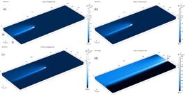
Heat flux on the plate surface, condition T7. For different laser travel times. (a) 0.3 s, (b) 0.4 s, (c) 0.5 s and (d) 1.08 s.

It is observed that for 0.3, 0.4, and 0.5 s, the highest temperature values are 4430 K, 4470 K, and 5950 K, respectively. The temperature varies as the laser beam advances along the Al/Ti interface, meaning the temperature is not constant at each time step. This variation is due to the interaction mechanisms between the beam and the material. The maximum simulated temperature occurs at the center of the heat source, on the titanium alloy side, where the laser beam was directed.

For the times shown in Figure 6(a), (b), and (c), three distinct regions can be observed, delineated by temperature ranges associated with the color scale: the molten region, on the aluminum alloy side, corresponds to the lightest blue shade. Similarly, the heat-affected zone (HAZ) exhibits the largest extent. Finally, the base metal, which was minimally affected by the heat input, is also highlighted.

It is also noted that the aluminum sheet exhibits a larger extent of HAZ. Figure 6 (d) shows the position of the laser 0.08 s after it has scanned the entire Al/Ti interface.

It should be noted that the thermocouples employed in this study provide a precision of 0.1 K but are limited to an operational range of approximately 1500 K. Therefore, experimental validation was restricted to the conduction and HAZ regions, where temperatures remained within this measurable range. The higher peak temperatures predicted in the molten pool and keyhole region (up to ~5950 K) cannot be directly validated with thermocouples. However, these values are consistent with reports in the literature for laser welding of titanium alloys, where vaporization and plasma formation occur³³.

Accordingly, while the experimental results confirm the accuracy of the model in the measurable domain (with discrepancies of only 2.5–6%), the predicted extreme values should be interpreted as model-based estimates beyond the limits of direct experimental validation. At this point, the highest heat flux is observed on the aluminum alloy side due to the thermal conductivity characteristics of the material (Figure 7).

Figure 7
Heat flux values on the sheet surface.

The welding energy and the offset value influenced the isotherms on both the aluminum alloy side and the titanium alloy side. Observing Figure 8, the isothermal contours on the top surface of the plate are shown for a time of 0.5 s, under conditions of the same offset and different heat inputs (HI) ((a) and (c)), and the same HI with different offsets ((a) and (b)). Note that the isotherms exhibit an elliptical shape and varying sizes. This is because the heat distribution fields calculated for each step were affected by the previous thermal energy. The elliptical shape also varies according to the welding speed and beam power for the same offset values.

Figure 8
Isotherms for conditions: (a) T5, (b) T1, (c) T7

For both the titanium and aluminum sheets, the isotherm is intense, and the temperature gradient is higher just ahead of the molten pool. On the other hand, due to the higher thermal conductivity of the aluminum alloy, the isotherms tend to be more circular.

The isotherms highlighted in Figure 9 show that the highest isotherm value is 4390 K, which is 40% higher than the boiling temperature of the Ti-6Al-4V³³ alloy, confirming the vaporization of elements from the titanium alloy. This satisfies the condition for plasma formation on the sheet surface due to the thermal load, leading to the subsequent formation of the keyhole.

Figure 9
Enlarged view of the isotherms for the welding condition of the sample for the T5 condition.

By comparing the simulated heat flow behavior with the previously presented microstructural transformations, it is confirmed that the isotherm duration and heating rate influenced grain growth³⁴. Furthermore, higher welding energy does not alter the shape but increases the size of the isotherm, thereby expanding the molten pool and the HAZ.

On the other hand, analyzing the isotherms on the titanium sheet side for the same beam displacement along the Al/Ti interface, and comparing conditions T6 and T9 (Figure 10), we observe that the temperature of isotherm I1 in T6 is 10% higher (539 K) than isotherm I2, observed under condition T9 (485 K). This indicates that for the same beam intensity and lower welding speed (T9), the heat dissipated by conduction in the titanium sheet was 22% lower than that transferred under condition T6, meaning more energy was absorbed by the titanium alloy in sample T9. This fact can be confirmed by Equation 12³⁵.

$P_D=4\rho t\left(T_m-T_m\right){\left(\frac{r.V_s}{k}/2\right)}^{1/3}$ (12)

The abbreviations presented in the equation above represent: $P_D$ - heat dissipated by conduction; $\lambda$ - thermal conductivity; $.V_s$ - welding speed; $.T_m$ - melting temperature plus an overheating of 200°C; $.T_e$ - ambient temperature; $r$ - radius of focus; $t$ - sheet thickness and $k$ - thermal diffusivity.

Figure 10
Isotherms for welding conditions: (a) T6 and (b) T9.

The heat treatment effect promoted during the thermal cycles generated in the welding process influences the metallurgical transformations of the molten pool and the heat-affected zone (HAZ). These transformations are fundamental in determining the mechanical properties of the weld. Therefore, modeling the thermal cycle and its relationship with welding energy and offset is of great importance.

Additionally, measuring the peak temperature and cooling rate experimentally is challenging due to the high temperatures and the narrow molten pool in the laser welding process. Thus, to validate the developed heat flow model, a comparison was made between the experimental and simulated thermal cycles.

As shown in Figure 11, the simulated thermal cycle is very close to the experimental values obtained using thermocouples. Two Type K thermocouples were used to measure the experimental thermal cycle, positioned on the titanium sheet surface at 2.0 mm from the heat source for both T6 and T9 conditions. The experimental thermal cycle values for T6 and T9 conditions were 6% and 2.5% higher, respectively, than the simulated results.

Figure 11
Comparison between experimental and simulated thermal cycles for the welding condition: (a) T6 and (b) T9.

These discrepancies are comparable to typical model-to-experiment differences reported for transient laser-welding simulations and are attributable to thermocouple response/attachment, millimeter-scale placement differences between sensor and model sampling point, literature-sourced temperature-dependent material properties, and modeling approximations (Gaussian heat source, simplified keyhole behavior).

In the predominantly elastic regime, thermal stress scales approximately with the local temperature rise (σ ≈ EαΔT), so a 2.5–6% thermal discrepancy yields a comparable first-order uncertainty in the elastic thermal stress contribution. Where plasticity and phase changes occur, non-linear effects and constitutive uncertainties can amplify residual-stress prediction uncertainty; conservatively, this can increase RS uncertainty to the order of several percent up to a few tens of percent locally. For the highest compressive residual stress observed (≈26 MPa), the thermal-error-propagated elastic uncertainty is ≈1–2 MPa; including model and material-property uncertainties gives a conservative uncertainty band of approximately ± (5–25%) of the predicted RS. To quantify sensitivity explicitly, a parametric uncertainty study (±2.5–6% perturbation of thermal input or material property values) is recommended for future work and is expected to confirm that the principal trends and process-optimization conclusions (e.g., influence of HI and offset on peak stress location and IMC thickness) remain robust.

Since residual stresses in laser welding primarily arise from constrained thermal contraction governed by the local thermal gradients and cooling rates, the validated thermal solution provides the required basis for predicting residual-stress distributions. Direct experimental residual-stress measurements were not available in the present study; therefore, stress results should be interpreted as model-based predictions whose accuracy is limited mainly by uncertainties in temperature-dependent elastoplastic properties and mechanical boundary conditions. Nevertheless, the model is suitable for assessing the relative influence of process parameters (HI and offset) on residual-stress trends and peak locations.

Figure 12 shows the positions of the points used to calculate the thermal cycles on the aluminum sheet side, specifically:

Figure 12
Position of points for calculations of simulated thermal cycles.

• P1: point located 1 mm from the interface,

• P2, P3, P4, and P5: sequentially positioned at 2 mm, 3 mm, 4 mm, and 5 mm from the joint interface.

Figure 13 presents the curves corresponding to the temperature variation over time for the five points located at different distances from the joint interface. These curves represent the simulated thermal cycles for the welding conditions in the following order: (a) T1, (b) T2, (c) T9, and (d) T12.Figure 13 shows that as the points move further from the joint interface, the peak temperature decreases rapidly, and the time required to reach it tends to increase. This occurs because the laser directly impacts the titanium alloy side, and heat propagates to the aluminum alloy primarily through conduction.

Figure 13
Simulated thermal cycles for welding conditions (aluminum sheet side): (a) T1, (b) T2, (c) T9 and (d) T12.

For an offset value of 0.5 mm, a 20% increase in welding energy resulted in nearly a 30% increase in the peak temperature (comparing conditions T1 and T2). However, with a 50% increase in welding energy, the heat source caused a 15% rise in the peak temperature (comparing conditions T9 and T12). The fact that the welding speed in conditions T9 and T12 was half the value used in conditions T1 and T2 explains the reduction by half in the peak temperature value.

Similarly, observing the cases with an offset of 0.3 mm, it is noted that a 20% increase in welding energy adds 6% to the maximum temperature value (comparing conditions T6 and T5). This behavior was also observed when comparing conditions T8 and T7.

On the other hand, Figure 14 shows the relationship between the cooling rate and the welding energy values, where T1, T2, T9, and T12 were analyzed for a 0.5 mm offset, and T5, T6, T7, and T8 for a 0.3 mm offset.

Figure 14
Cooling rate related to heat input values.

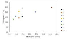
The cooling rate (CR) was calculated based on Equation 13, considering the peak temperature at Point 2 (2 mm from the Al/Ti interface) for each welding condition, and using the thermophysical properties of the aluminum alloy.

$\frac{dT}{dt}=2\pi k\rho c_p{\left(\frac{u_{x}h}{q}\right)}^2{\left(T-T_0\right)}^3$ (13)

Regarding Figure 14, for the condition with a 0.5 mm offset, it was observed that a 20% increase in heat input (HI) resulted in an 11.2% increase in the cooling rate (CR). However, the same HI increase led to a 16.5% rise in CR for a 0.3 mm offset. Additionally, for smaller offset values and the same HI, an increase in CR was noted. This occurred because the point under analysis was closer to the heat source.

The different HI values and offsets influenced the cooling rate and peak temperature. Higher HI values during laser welding resulted in increased cooling rates (as shown in Figure 14). In other words, there was a rapid temperature drop over a short time for lower welding energy values. Consequently, a narrower weld profile with a smaller HAZ was produced.

The cooling rate and peak temperature also affected the volumetric fraction of precipitates formed in the molten pool of the aluminum alloy. The volumetric fraction of precipitates was calculated using the ImageJ^® image processing software. As observed in Figure 15, higher cooling rates contributed to the formation of a greater volumetric fraction of precipitates.

Figure 15
Relationship between cooling rate and volume fraction of precipitates.

3.2. Effect heat flow and cooling rate on the formation of intermetallic compounds

Similarly, the developed model for simulating heat input, after being validated, contributed to explaining the mechanisms of intermetallic compound layer formation at the Al/Ti interface and the potential metallurgical weldability of the dissimilar joint.

First, the peak temperature was simulated at 0.06 mm from the joint interface (Figure 16) since this distance (approximately) corresponds to where the formation of the intermetallic compound layer was observed, for example, under condition T1. The maximum temperature in the analyzed region was 900 K (Figure 17), resulting in a cooling rate of 337.76 °C/s.

Figure 16
Point position for the simulated temperature peak at 0.06 mm from the Al/Ti interface, condition T1.

Figure 17
Thermal cycle simulated at 0.06 mm from the Al/Ti interface, condition T1.

The relationship between cooling rate and intermetallic compound formation during laser welding was elucidated through a thermodynamic analysis of the phases present. The Gibbs free energy ΔG_f

of the intermetallic compounds TiAl and $T{i}_{3}Al$ was highlighted within the temperature range of 273 to 1473 K, governed by the formation law presented in Table 5³⁶.

Table 5
Gibbs free energy of formation for TiAl and $T{i}_{3}Al$.

Intermetallic compound	Free energy of formation ($\Delta G_f$
${\text{Ti}}_3\text{Al}$	-29633,6 + 6,708017T
$\text{TiAl}$	-37445,1 + 16,79376T

Figure 18 shows the Gibbs free energy behavior for the two aforementioned phases. It can be observed that the Gibbs free energy of the $T{i}_{3}A$ phase is lower than that of the TiAl phase. Due to the rapid cooling rate in the laser welding process, the phase transition tends to occur in a manner that minimizes the system's energy³⁶.

Figure 18
Gibbs free energy of formation for TiAl and $T{i}_{3}Al$.

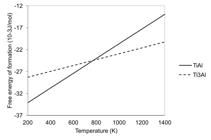
The Ti-Al phase diagram³⁷ indicates that the $\alpha \to {\alpha }_2+\gamma$ process occurs at temperatures above 774.5 K. The simulated temperature for the region of interest was 900 K, enabling this reaction. However, as shown in Figure 18 the Gibbs free energy for $T{i}_{3}Al$ formation is lower than the Gibbs free energy for TiAl formation (at 1400 K). Therefore, there is a tendency for the formation of the ${\alpha }_2-T{i}_{3}Al$.

In other words, the difference in Gibbs free energy between the ${\alpha }_2$ and $\gamma$ phases favor the formation of the ${\alpha }_2$ phase at high cooling rates. This behavior likely explains why the Ti-Al phase was identified in only three out of the twenty-four analyzed points.

Additionally, it was observed that increasing the cooling rate, while maintaining the same offset, reduced the thickness of the intermetallic compound (IMC) layer. Figure 19 illustrates this finding. It is noted that a 50% increase in heat input (from 9.6 to 14.4 J/mm) resulted in a nearly 50% reduction in the IMC layer thickness (from 7 µm to 3 µm).

Figure 19
IMC layer thickness: (a) Cooling rate = 16 °C/s, HI = 9.6 J/mm – condition T7. (b) Cooling rate = 24 °C/s, HI = 14.4 J/mm – condition T5.

The predicted intermetallic compound (IMC) thicknesses are directly relevant to the mechanical performance of the dissimilar joint. Previous studies have reported that thin IMC layers (<5 µm) generally contribute to sound metallurgical bonding, whereas excessive IMC growth (>10 µm) promotes brittle fracture and significantly reduces tensile and shear strength³⁸. This correlation highlights the practical significance of controlling process parameters such as heat input and offset, not only for thermal management but also for optimizing the structural integrity of Ti/Al dissimilar welds in aerospace applications.

The transient heat flow that influenced the formation of intermetallics originated from the heat transferred by conduction ($d_{flux}$) from the titanium alloy side to the aluminum alloy side. The $d_{flux}$ calculated using Equation 14, was affected by the heat input (HI) and offset for each welding condition, as shown in Figure 20.

$d_{flux}={\left(k_i{\nabla }^{2}T\right)}^{\frac{1}{2}}$ (14)

Where $k_i$ represents the thermal conductivity, in W/mK.

Figure 20
Heat flux profile for conditions: T1 (14.4 J/mm, 0.5 offset). T5 (14.4 J/mm, 0.3 offset), T7 (9.6 J/mm, 0.3 offset), T6 (12.0 J/mm, 0.3 offset), and T9 (24 J/mm, 0.5 offset).

Figure 20 indicates that the maximum heat flux values for conditions T1, T5, and T6 were obtained within the same time intervals, as these conditions had the same welding speed. However, condition T5 resulted in a heat flux 20.6% higher than that generated by condition T6 due to the higher HI value. The lower heat flux for condition T1 was attributed to the larger offset (compared to T5).

On the other hand, the leftward shift of the heat flux curve for condition T7 was due to its higher welding speed (50 mm/s). Comparing T1 and T9, the heat flux values were observed to be very similar.

Although the HI for T9 was 66% higher than for T1, and both conditions had the same offset values, the $d_{flux}$ was expected to be higher for the condition with greater HI (as previously analyzed). However, the region of interest reached a temperature of 1175 K (above the titanium allotropic transformation temperature of 1155 K³⁹), where a reduction in titanium’s thermal conductivity occurred (Figure 21).

Figure 21
Temperature values at point 1Al for conditions T1, T5, T6, T7 and T9.

3.3. Simulation of residual stresses (RS) in the welded joint

Residual stresses (RS) can significantly affect the welded joint. For instance, they can compromise fatigue resistance, induce brittle fracture, and promote stress corrosion. Therefore, one of the factors responsible for failures in dissimilar joints is the presence of RS. Residual stresses are generated within the material due to non-uniform plastic and elastic deformations, primarily caused by temperature variations. In the case of laser welding, the localized high energy is the primary source of RS⁴⁰.

The literature shows that most modeling studies on residual stresses in welded joints have not considered the influence of phase transformations⁴¹-⁴⁵. This is because the expansion caused by martensitic transformation is negligible compared to the stresses arising from thermal deformations. The present modeling approach for RS also prioritized the occurrence of the most significant phenomena.

Figure 22 presents the principal stress distribution on the titanium alloy side starting from the Al/Ti interface. It is observed that residual stresses decrease as the analyzed points move farther from the heat source. Furthermore, it is evident that tensile and compressive RS are distributed differently for conditions T1 and T5. Despite having the same HI values, these conditions have different offset values.

Figure 22
Distribution of first principal stresses on the titanium alloy side

Condition T5, with an offset of 0.3 mm, exhibited compressive stress values of 620 MPa because the analyzed point was located within the HAZ (closer to the molten pool). This scenario did not occur for condition T1 (offset of 0.5 mm), where only tensile RS (1000 MPa) were observed, indicating that the point is located within the molten pool.

In line with the presented results, both the offset and the welding heat input (HI) significantly affected the residual stresses (RS) generated in the weld region. Comparing the RS results for the titanium side and the aluminum side (Figure 22 and Figure 23, respectively), a considerable difference in the values and distribution of RS between the titanium alloy and aluminum alloy is observed. This difference arises due to the distinct thermophysical properties and microstructural transformations of the two alloys. Additionally, the laser directly impacted the titanium alloy, and the heat flow was primarily transferred to the aluminum alloy through conduction.

Figure 23
Distribution of first principal stresses on the aluminum alloy side. (a) offset = 0.3 mm; (b) offset = 0.5 mm

In general, Figure 23(a) shows that as HI increases, the residual stress values also increase. However, Figure 23(b) reveals that a 16% increase in HI did not result in significant changes in RS, indicating that an offset of 0.5 mm suppressed the generation of residual stresses. Nevertheless, for the condition with the highest HI (24 J/mm), the maximum RS value (~26 MPa) was reached and remained almost constant. It is noteworthy that this welding condition resulted in a larger molten pool.

Principal stresses were used to estimate regions with compressive stresses (negative values) and tensile stresses (positive values). Principal stress refers to the stress vector perpendicular to the plane, where shear stresses are not considered. In Figure 23(a), for the condition with a 0.3 mm offset, the thermal cycle generated by an HI of 14.0 J/mm produced a tensile residual stress of approximately 25 MPa at a point 0.5 mm away from the Al/Ti interface. However, for the condition with a 0.5 mm offset, under the same HI and at the same distance from the Al/Ti interface, a compressive residual stress of 15 MPa was observed (Figure 23(b)).

The first scenario indicates that the analyzed region corresponds to the molten pool, while the second case refers to the heat-affected zone (HAZ), which exhibits compressive residual stresses due to the expansion of the liquid metal. These observations are supported by microstructural images of these regions, as documented in the work of Ribeiro et al.¹.

The condition with an HI of 24 J/mm and an offset of 0.5 mm resulted in a maximum deformation of 0.09 mm on the aluminum sheet side. The 50% increase in deformation for the aluminum alloy is consistent, as its thermal expansion is nearly twice that of the titanium alloy. This also indicates that the offset values used did not influence the thermal deformation on the aluminum side, which was affected solely by the welding energy.

Similarly, the predicted deformation of the titanium sheet induced by thermally generated stresses was evaluated for conditions T5, T7, and T9. Notably, even at the highest heat input (HI) of 24 J/mm (condition T9), the maximum titanium-sheet distortion was only 0.07 mm. This result indicates that, within the investigated process window, variations in HI and offset had a limited effect on titanium-sheet distortion. It is important to reiterate that in the development of this model, the sheets were considered fixed. In scenarios where the restraining force is removed, transverse and longitudinal residual stresses induce greater displacement and, consequently, increased distortion of the sheets²⁷. Conversely, the constraints imposed on the sheets lead to a 16% increase in RS values⁴⁶.

For conditions with the same offset but different HI values, for example, T2 (12.0 J/mm), T1 (14.4 J/mm), and T9 (24.0 J/mm), it was observed that a 20% increase in HI did not significantly affect the behavior of the principal stresses. However, a 200% increase in welding energy (comparing T9 with T2) resulted in 255 MPa of compressive stress, whereas condition T2 exhibited 1020 MPa of tensile residual stress.

It is important to highlight that the lower welding speed in condition T9 led to a higher HI. Consequently, the reduction in welding speed contributed to an increase in residual stresses due to the greater energy absorbed per unit length.

4. Conclusions

This study developed and validated a multiphysical finite element model to simulate heat flux and residual stress distribution in AA6013/Ti-6Al-4V dissimilar joints welded by laser beam. The simulation results correlated strongly with experimental thermal cycles, with deviations of 2.5–6%, confirming the accuracy of the developed approach.

The findings highlight that welding speed, heat input, and offset are critical parameters in determining joint performance. For the same beam intensity, reducing the welding speed (T9 compared to T6) decreased heat dissipation in titanium by 22%, resulting in higher energy absorption. Residual stress analysis revealed that values decrease with distance from the laser beam and that a 0.2 mm variation in offset did not significantly affect stresses for the same HI. However, for a fixed offset, increasing HI led to higher residual stresses, with a maximum compressive stress of 26 MPa (≈10% of the AA6013 yield strength) observed at HI = 24 J/mm. Additionally, the cooling rate was shown to play a decisive role in IMC layer control, as higher cooling rates reduced IMC thickness from 7 µm to 3 µm, enhancing weldability.

The findings suggest that controlling HI and welding speed is essential to minimize residual stresses and limit IMC growth, both of which are critical for aerospace-grade dissimilar joints. Specifically, intermediate HI values combined with appropriate offsets yield lower stress concentrations without compromising metallurgical bonding. Thin IMC layers (<5 µm), achieved under higher cooling rates, are particularly beneficial in improving tensile and fatigue performance in service. These insights provide practical guidelines for optimizing laser welding of Ti/Al joints used in aerospace structures.

Additionally, the study revealed that the cooling rate plays a critical role in the formation of intermetallic compounds at the Al/Ti interface. Higher cooling rates promoted the formation of the Ti₃Al phase over the TiAl phase, as the Gibbs free energy of Ti₃Al was lower, making it more thermodynamically favorable. Additionally, increasing the heat input reduced the thickness of the IMC layer, which is beneficial for joint integrity.

The developed models can be used to estimate joint regions, intermetallic compound (IMC) formation, and the mechanical properties of the dissimilar joint (AA6013/Ti-6Al-4V) welded by a laser beam, providing valuable insights for optimizing the welding process in aerospace applications. Future developments should incorporate additional physical phenomena into the model to further enhance predictive accuracy. Coupling fluid flow within the molten pool and keyhole dynamics would improve the description of heat and mass transport. Integrating phase transformation kinetics and cyclic mechanical testing would also help establish a more comprehensive framework to link microstructural evolution with long-term mechanical performance.

• Data Availability
  The data that support the findings of this study are available from the corresponding author upon reasonable request.

5. References

• ¹ Ribeiro ACN, de Siqueira RHM, de Lima MSF, Giorjão RAR, Abdalla AJ. Improvement weldability of dissimilar joints (Ti-6Al-4V/Al6013) for aerospace industry by laser beam welding. Int J Adv Manuf Technol. 2021;116(3-4):1053-70. https://doi.org/10.1007/s00170-021-07506-4
  » https://doi.org/10.1007/s00170-021-07506-4
• ² Biswas AR, Banerjee N, Sen A, Maity SR. Applications of laser beam welding in automotive sector-a review. In: Ramesh Babu N, Kumar S, Thyla PR, Sripriyan K, editors. Advances in additive manufacturing and joining. Singapore: Springer; 2023. p. 37-46. https://doi.org/10.1007/978-981-19-7612-4_4
  » https://doi.org/10.1007/978-981-19-7612-4_4
• ³ Rosenthal D. Mathematical theory of heat distribution during welding and cutting. Welding Journal. 1941;20:220-34.
• ⁴ Andrew M. Numerical simulations of thermal processes and welding. Essex: University of Essex; 2003.
• ⁵ Mackwood AP, Crafer RC. Thermal modelling of laser welding and related processes: a literature review. Opt Laser Technol. 2005;37(2):99-115. https://doi.org/10.1016/j.optlastec.2004.02.017
  » https://doi.org/10.1016/j.optlastec.2004.02.017
• ⁶ Johnson TE. Multiphysical modeling in laser welding: current advances and future directions. Comput Mater Sci. 2017;132:125-40.
• ⁷ Otto A, Schmidt M. Towards a universal numerical simulation model for laser material processing. Phys Procedia. 2010;5:35-46. https://doi.org/10.1016/j.phpro.2010.08.120
  » https://doi.org/10.1016/j.phpro.2010.08.120
• ⁸ Unverdi SO, Tryggvason G. A front-tracking method for viscous, incompressible, multi-fluid flows. J Comput Phys. 1992;100(1):25-37. https://doi.org/10.1016/0021-9991(92)90307-K
  » https://doi.org/10.1016/0021-9991(92)90307-K
• ⁹ Pang S, Chen W, Wang W. A quantitative model of keyhole instability induced porosity in laser welding of titanium alloy. Metall Mater Trans, A Phys Metall Mater Sci. 2014;45(6):2808-18. https://doi.org/10.1007/s11661-014-2231-3
  » https://doi.org/10.1007/s11661-014-2231-3
• ¹⁰ Lu F, Li X, Li Z, Tang X, Cui H. Formation and influence mechanism of keyhole-induced porosity in deep-penetration laser welding based on 3D transient modeling. Int J Heat Mass Transf. 2015;90:1143-52. https://doi.org/10.1016/j.ijheatmasstransfer.2015.07.041
  » https://doi.org/10.1016/j.ijheatmasstransfer.2015.07.041
• ¹¹ Dal M, Fabbro R. [INVITED] An overview of the state of art in laser welding simulation. Opt Laser Technol. 2016;78:2-14. https://doi.org/10.1016/j.optlastec.2015.09.015
  » https://doi.org/10.1016/j.optlastec.2015.09.015
• ¹² Dyadechko V, Shashkov M. Moment-of-fluid interface reconstruction. Math Model Anal. 2005;836:1-41.
• ¹³ Zeng Y, Yang J, Dou T, Zheng M, Zhao Y, Oliveira JP, et al. Influence of laser powder bed fusion of high-entropy alloy transition layer on the wetting and spreading behaviour of Al alloy on steel substrate surface. J Mater Process Technol. 2025;340:118872. https://doi.org/10.1016/j.jmatprotec.2025.118872
  » https://doi.org/10.1016/j.jmatprotec.2025.118872
• ¹⁴ ASTM International. ASTM B265-15: standard specification for titanium and titanium alloy strip, sheet, and plate. West Conshohocken: ASTM; 2015.
• ¹⁵ Zhang CQ, Robson JD, Prangnell PB. Dissimilar ultrasonic spot welding of aerospace aluminum alloy AA2139 to titanium alloy TiAl6V4. J Mater Process Technol. 2016;231:382-8. https://doi.org/10.1016/j.jmatprotec.2016.01.008
  » https://doi.org/10.1016/j.jmatprotec.2016.01.008
• ¹⁶ Braun R. Laser beam welding of Al-Mg-Si-Cu alloy 6013 sheet using silicon rich aluminium filler powders. Mater Sci Technol. 2005;21(1):133-40. https://doi.org/10.1179/174328405X16225
  » https://doi.org/10.1179/174328405X16225
• ¹⁷ de Siqueira RHM, de Oliveira AC, Riva R, Abdalla AJ, Baptista CARP, de Lima MSF. Mechanical and microstructural characterization of laser-welded joints of 6013-T4 aluminum alloy. J Braz Soc Mech Sci Eng. 2014;37(1):133-40. https://doi.org/10.1007/s40430-014-0175-6
  » https://doi.org/10.1007/s40430-014-0175-6
• ¹⁸ ASTM International. ASTM B381-13: standard specification for titanium and titanium alloy forgings. West Conshohocken: ASTM; 2013.
• ¹⁹ COMSOL Multiphysics. Introduction to COMSOL multiphysics [online]. COMSOL, Inc.; 2023 [cited 2025 Jan 15]. Available from: https://www.comsol.com/documentation
  » https://www.comsol.com/documentation
• ²⁰ Indhu R, Loganathan S, Vijayaraghavan L, Soundarapandian S. A study on continuous beam laser welding of dissimilar materials using multi-physics simulation. In: Proceedings of the 2018 COMSOL Conference; 2018; Bangalore, India. Proceedings. Burlington (MA): COMSOL; 2018.
• ²¹ Elijah Kannatey-Asibu J. Principles of laser materials processing. London: John Wiley & Sons, Inc; 2009. https://doi.org/10.1002/9780470459300
  » https://doi.org/10.1002/9780470459300
• ²² Volpp J, Vollertsen F. Modeling keyhole oscillations during laser deep penetration welding at different spatial laser intensity distributions. Prod Eng. 2015;9(2):167-78. https://doi.org/10.1007/s11740-014-0594-3
  » https://doi.org/10.1007/s11740-014-0594-3
• ²³ Ribeiro ACN. Optimization of the weldability of dissimilar AA6013/Ti6Al4V joints for aerospace applications obtained by laser welding [dissertation]. São José dos Campos: Division of Space Science and Technology, Instituto Tecnológico de Aeronáutica; 2022 [cited 2025 Oct 9]. Available from: http://www.bdita.bibl.ita.br/tesesdigitais/lista_resumo.php?num_tese=78575
  » http://www.bdita.bibl.ita.br/tesesdigitais/lista_resumo.php?num_tese=78575
• ²⁴ Bonacina C, Comini G, Fasano A, Primicerio M. Numerical solution of phase-change problems. Int J Heat Mass Transfer. 1973;16(10):1825-32. https://doi.org/10.1016/0017-9310(73)90202-0
  » https://doi.org/10.1016/0017-9310(73)90202-0
• ²⁵ Tomashchuk I, Bendaoud I, Sallamand P, Cicala E, Lafaye S, Almuneau M. Multiphysical modelling of keyhole formation during dissimilar laser welding. In: 2016 COMSOL Conference; 2016 Oct 12-14; Franche-Comté, France. Proceedings. Munich, Germany: COMSOL; 2016. p. 1-7.
• ²⁶ Aycock KN, Campelo SN, Davalos RV. A comparative modeling study of thermal mitigation strategies in irreversible electroporation treatments. J Heat Transfer. 2022;144(3):031206. https://doi.org/10.1115/1.4053199 PMid:35833151.
  » https://doi.org/10.1115/1.4053199
• ²⁷ Leitz K-H. Thermo-mechanical modelling of laser beam welding of molybdenum. In: 2018 COMSOL Conference; Oct 2018; Lausanne, Switzerland. Proceedings. Burlington (MA): COMSOL; 2018. p. 1-7.
• ²⁸ Jiang W, Luo Y, Li JH, Woo W. Residual stress distribution in a dissimilar weld joint by experimental and simulation study. J Press Vessel Technol. 2017;139(1):1-10. https://doi.org/10.1115/1.4033532
  » https://doi.org/10.1115/1.4033532
• ²⁹ von Mises R. Mechanik der festen Körper im plastisch deformablen Zustand. Göttinger Nachrichten für Mathematik und Physik. 1913;1:582-92.
• ³⁰ Aakash BS, Connors JP, Shields MD. Stress-strain data for aluminum 6061-T651 from 9 lots at 6 temperatures under uniaxial and plane strain tension. Data Brief. 2019;25:104085. https://doi.org/10.1016/j.dib.2019.104085 PMid:31304211.
  » https://doi.org/10.1016/j.dib.2019.104085
• ³¹ Maxim Integrated Products. Cold-Junction-Compensated K-Thermocouple-to-Digital Converter (0°C to +1024°C) [Internet]. Sunnyvale, CA, USA; 2002 [cited 2025 Oct 9]. Available from: https://www.alldatasheet.com/datasheet-pdf/pdf/73692/MAXIM/MAX6675.html
  » https://www.alldatasheet.com/datasheet-pdf/pdf/73692/MAXIM/MAX6675.html
• ³² Bertoleti P. Como usar o termopar tipo K com Arduino [Internet]. Maker Hero; 2020 [cited 2025 Oct 9]. Available from: https://www.makerhero.com/blog/como-usar-o-termopar-tipo-k-com-arduino/?srsltid=AfmBOora-1p8VNT9MzjSlnEIPJ5j7BDbkS38l9t1M5Od8O9PTN6Bvlus
  » https://www.makerhero.com/blog/como-usar-o-termopar-tipo-k-com-arduino/?srsltid=AfmBOora-1p8VNT9MzjSlnEIPJ5j7BDbkS38l9t1M5Od8O9PTN6Bvlus
• ³³ Bremen S, Meiners W, Diatlov A. Elemental vaporization of Ti-6Al-4V in selective laser melting. Laser Tech J. 2012;9(2):33-8. https://doi.org/10.1002/latj.201290018
  » https://doi.org/10.1002/latj.201290018
• ³⁴ Alhazaa AN, Khan TI. Diffusion bonding of Al7075 to Ti-6Al-4V using Cu coatings and Sn-3.6Ag-1Cu interlayers. J Alloys Compd. 2010;494(1-2):351-8. https://doi.org/10.1016/j.jallcom.2010.01.037
  » https://doi.org/10.1016/j.jallcom.2010.01.037
• ³⁵ Bergmann JP, Patschger A, Bastick A. Enhancing process efficiency due to high focusing with high brightness lasers - applicability and constraints. Phys Procedia. 2011;12:66-74. https://doi.org/10.1016/j.phpro.2011.03.009
  » https://doi.org/10.1016/j.phpro.2011.03.009
• ³⁶ Kattner UR, Lin JC, Chang YA. Thermodynamic assessment and calculation of the Ti-Al system. Metall Trans, A, Phys Metall Mater Sci. 1992;23A(8):2081-90. https://doi.org/10.1007/BF02646001
  » https://doi.org/10.1007/BF02646001
• ³⁷ Massalski TB, Murray JL, Bennet LH. Binary alloy phase diagrams. Vol. 1. Materials Park: ASM International; 1986.
• ³⁸ Bunaziv I, Akselsen OM, Ren X, Nyhus B, Eriksson M, Gulbrandsen-Dahl S. A review on laser-assisted joining of aluminium alloys to other metals. Metals. 2021;11(11):1680. https://doi.org/10.3390/met11111680
  » https://doi.org/10.3390/met11111680
• ³⁹ Liu S, Chew Y, Weng F, Sui S, Du Z, Man Y, et al. Effects of laser pulse modulation on intermetallic compounds formation for welding of Ti-6Al-4V and AA7075 using AA4047 filler. Mater Des. 2022;213:110325. https://doi.org/10.1016/j.matdes.2021.110325
  » https://doi.org/10.1016/j.matdes.2021.110325
• ⁴⁰ Joseph A, Rai SK, Jayakumar T, Murugan N. Evaluation of residual stresses in dissimilar weld joints. Int J Press Vessels Piping. 2005;82(9):700-5. https://doi.org/10.1016/j.ijpvp.2005.03.006
  » https://doi.org/10.1016/j.ijpvp.2005.03.006
• ⁴¹ Panda SK, Kuntz ML, Zhou Y. Finite element analysis of effects of soft zones on formability of laser welded advanced high strength steels. Sci Technol Weld Join. 2009;14(1):52-61. https://doi.org/10.1179/136217108X343920
  » https://doi.org/10.1179/136217108X343920
• ⁴² Xie P, Zhao HY, Wu B, Gong SL. Using finite element and contour method to evaluate residual stress in thick Ti-6Al-4V alloy welded by electron beam welding. Acta Metall Sin. 2015;28(7):922-30. https://doi.org/10.1007/s40195-015-0276-y
  » https://doi.org/10.1007/s40195-015-0276-y
• ⁴³ Liu C, Zhang J, Niu J. Numerical and experimental analysis of residual stresses in full-penetration laser beam welding of Ti-6Al-4V alloy. Rare Met Mater Eng. 2009;38(8):1317-20. https://doi.org/10.1016/S1875-5372(10)60066-5
  » https://doi.org/10.1016/S1875-5372(10)60066-5
• ⁴⁴ Tremarin RC, Pravia ZMC. Analysis of the influence of residual stress on fatigue life of welded joints. Lat Am J Solids Struct. 2020;17(3):1-26. https://doi.org/10.1590/1679-78256020
  » https://doi.org/10.1590/1679-78256020
• ⁴⁵ Deng D, Liu X, He J, Liang W. Investigating the influence of external restraint on welding distortion in thin-plate bead-on joint by means of numerical simulation and experiment. Int J Adv Manuf Technol. 2016;82(5-8):1049-62. https://doi.org/10.1007/s00170-015-7413-7
  » https://doi.org/10.1007/s00170-015-7413-7
• ⁴⁶ Smith WF, Hashemi J. Fundamento de engenharia e ciência dos materiais. São Paulo: AMGH; 2012.

Edited by

• Associate Editor:
  José Daniel Biasoli de Mello.

• Editor-in-Chief:
  Luiz Antonio Pessan.

Data availability

The data that support the findings of this study are available from the corresponding author upon reasonable request.

Publication Dates

• Publication in this collection
  17 Apr 2026
• Date of issue
  2026

History

• Received
  14 Oct 2025
• Reviewed
  30 Jan 2026
• Accepted
  08 Mar 2026