MONITORING TEMPORARY CROPS IN IPU-CE USING SAR TIME SERIES IMAGES AND MACHINE LEARNING

MONITORAMENTO DE CULTIVOS TEMPORÁRIOS EM IPU-CE UTILIZANDO IMAGENS DE SÉRIES TEMPORAIS SAR E APRENDIZADO DE MÁQUINA

SURVEILLANCE DES CULTURES TEMPORAIRES DANS IPU-CE À L'AIDE D'IMAGES DE SÉRIES CHRONOLOGIQUES SAR ET D'APPRENTISSAGE AUTOMATIQUE

Abstract

In recent decades, remote sensing techniques have advanced considerably, enabling effective monitoring of land use, agricultural productivity, and the environmental impacts of agricultural expansion in the Caatinga biome. This study integrates H-αlpha decomposition products developed by Cloude-Pottier, Sigma-0 backscatter, polarization ratio, and vegetation indices derived from Sentinel-1 data cube from July 2021 to August 2022. The methodological approach enhanced the quality and heterogeneity of training samples, resulting in a more accurate and spatially distributed classified map. These findings contribute to a deeper understanding of agricultural dynamics in Ipu-CE, especially in areas with multiple crop cycles, and provide valuable insights to support sustainable agricultural monitoring and policymaking in semi-arid regions.

Keywords:
Monitoring Land Use and Land Cover; SAR Data Cubes; Caatinga Biome

Resumo

Nas últimas décadas, as técnicas de sensoriamento remoto avançaram consideravelmente, permitindo o monitoramento eficaz do uso da terra, da produtividade agrícola e dos impactos ambientais da expansão agrícola no bioma Caatinga. Este estudo integra produtos de decomposição H-alpha desenvolvidos por Cloude-Pottier, retroespalhamento Sigma-0, razão de polarização e índices de vegetação derivados de dados Sentinel-1 em um cubo de dados abrangendo julho de 2021 a agosto de 2022. A abordagem metodológica melhorou a qualidade e a heterogeneidade das amostras de treinamento, resultando em um mapa de classificação mais preciso e espacialmente distribuído. Essas descobertas contribuem para uma compreensão mais profunda da dinâmica agrícola em Ipu-CE, especialmente em áreas com múltiplos ciclos de cultivo, e fornecem insights valiosos para apoiar o monitoramento agrícola sustentável e a formulação de políticas em regiões semi-áridas.

Palavras-chave:
Monitoramento do Uso e Cobertura da Terra; Cubos de Dados SAR; Bioma Caatinga

Résumé

Au cours des dernières décennies, les techniques de télédétection ont considérablement progressé, permettant une surveillance efficace de l'utilisation des terres, de la productivité agricole et des impacts environnementaux de l'expansion agricole dans le biome de la Caatinga. Cette étude intègre les produits de décomposition H-alpha développés par Cloude-Pottier, la rétrodiffusion Sigma-0, le rapport de polarisation et les indices de végétation dérivés des données Sentinel-1 dans un cube de données couvrant la période de juillet 2021 à août 2022. L'approche méthodologique a amélioré la qualité et l'hétérogénéité des échantillons d'entraînement, ce qui a donné lieu à une carte de classification plus précise et plus distribuée spatialement. Ces résultats contribuent à une meilleure compréhension de la dynamique agricole dans l'Ipu-CE, en particulier dans les zones à cycles de cultures multiples, et fournissent des informations précieuses pour soutenir la surveillance et l'élaboration de politiques agricoles durables dans les régions semi-arides.

Mots-clés:
Surveillance de l'utilisation et de la couverture terrestre; cubes de données SAR; biome de Caatinga

INTRODUCTION

Synthetic aperture radars (SAR) are remote sensing systems that use microwave pulses to capture high-resolution images of the Earth’s surface and record the signal backscattered by targets, allowing the identification of their characteristics [Paradella et al. 2009]. Unlike optical sensors, it can collect data under meteorological and lighting conditions once SAR penetrates clouds, vegetation, and rain and operates at night [Le Toan and Floury 1998]. SAR emits energy pulses in the microwave range. It makes SAR images useful for continuous environmental monitoring applications [Moreira et al. 2013], [Kasischke et al. 1997], [Diniz et al. 2022]. These characteristics and processing derived from SAR images, such as Ground Range Detected (GRD), vegetation index, covariance matrix, polarimetric decomposition, and band ratio, allow SAR to provide valuable information about the surface despite some limitations, such as ionospheric effects and data availability [Gama et al. 2022], [Ulaby et al. 1982].

The increase in open data availability and application of remote sensing technologies in agriculture has transformed how crops are monitored and managed. Using time series and data cubes has become particularly prominent among the strategies available, as it effectively captures the temporal evolution of agricultural landscapes [Adami et al. 2012]. These methodologies are vital for crop mapping, offering a thorough and precise representation of land use and cover changes. Despite the potential methodologies and available data, as Sentinel-1 [European Space Agency 2022], there are few studies in Caatinga Biome1, especially in land use and land cover (LULC) monitoring. However, the Brazilian Chamber of Deputies is considering a bill to establish the National Policy for the Recovery of Caatinga Vegetation [Brazil 2024], which was already approved unanimously in the Federal Senate. This would aggregate efforts to monitor the Biome.

In this sense, we aimed to monitor and understand the dynamics of agricultural activity in Ipu, Ceará, in the Brazilian Caatinga Drought Polygon [Markham 1967]. We processed Sentinel-1 images from the regions around Ipu-CE from Jul/2021 to Aug/2022 and used time series and data cube methodologies to enhance temporary crops. Additionally, we investigated the SAR features used to improve the classification. We use previous knowledge about the study area, farmer information, field images, and statistical analyses to validate the classes obtained from our results. The product has the potential to support the implementation of public policies for sustainable agriculture. It contributes to the improvement of monitoring with less atmospheric interference.

BACKGROUND

SAR data provides detailed information on the structure and composition of the Earth’s surface by receiving microwave pulses reflected from targets. Sentinel-1A is one of large scale open data available in level 0, 1 and 2 for users application [ESA 2024]. There are some processes that should be applied to extract SAR features from Sentinel-1A, as thermal noise removal, radiometric calibration, geometric correction, speckle filtering, and polarimetric decomposition are essential steps in SAR image processing. Radiometric calibration adjusts radar return values to reflect surface properties correctly [López Martinez 2003]. Geometric correction ensures spatial data accuracy by correcting geographic distortions in the image through image modification [Hanssen 2001]. Speckle filtering is essential to reduce the characteristic noise of SAR images. Filters such as Lee, Frost, and Gamma MAP are widely used [Lee et al. 1994]. Speckle is a granular noise inherent in SAR images due to the coherent nature of the radiation used. Several filters mitigate this noise while keeping the image information intact. The Lee filter, which smooths speckles by maintaining edges using a statistical approach, is among the most popular.

Polarimetric decomposition is a method that splits the SAR signal into parts that represent various scattering mechanisms, including volumetric, double, and single scattering. H-alpha decomposition is a polarimetric approach that aims to find and quantify scattering components represented by eigenvectors and eigenvalues [Cloude and Pottier 1996]. Unlike the result for quadrature polarization images, the result for dual polarization images is significant only for Entropy (H) and Alpha Angle (α), discarding Anisotropy (A). With this range of features, SAR has a number of applications, including monitoring deforestation [Doblas et al. 2020], agriculture [Tomppo et al. 2019], water resource management [Liao et al. 2020] and studying natural disasters [Barra et al. 2016]. For example, the health of agricultural crops is monitored, changes in forest cover are mapped and floods are detected with SAR data [ESA 2024, Sano et al. 2023].

The analysis of satellite image time series allows the detection of changes in the earth’s surface over time, enabling the mapping of seasonal and interannual patterns in vegetation and the identification of transitions between different land uses [Pelletier et al. 2019]. Despite of the few studies in Caatinga biome, this technique is widely used in the Cerrado to monitor agricultural expansion, deforestation, and the recovery of degraded areas, providing crucial information for environmental management and territorial planning [Simões et al. 2020, Picoli et al. 2018, Sano et al. 2007].

Data cubes are used to perform time series classifications because their structured format organizes multi-dimensional remote sensing images, enabling the efficient analysis of large volumes of data [Truckenbrodt et al. 2019]. Researchers use data cubes to detect changes over time and extract relevant information for various applications, such as agricultural monitoring, land use studies, and environmental phenomenon analysis [Ferreira et al. 2020]. Satellite image time series are particularly effective in regions like Caatinga, where native vegetation and agricultural areas exist alongside one another in a complex landscape. Utilizing this approach aids in identifying subtle changes in land cover and monitoring annual agricultural cycles, ultimately contributing to sustainable agriculture and environmental conservation [Simões et al. 2020].

Machine learning (ML) algorithms, such as Random Forest (RF), are widely utilized for LULC classification. ML methodologies have demonstrated effectiveness in classifying multitemporal images, thanks to their capability to process large datasets and capture the intricacies of land use transitions [Pelletier et al. 2016]. Although there are some LULC products for Caatinga [Ganem et al. 2020], those remain mainly limited to optical images. When applied to time series SAR images, these techniques facilitate the identification of distinct crop phenological patterns, aiding in the differentiation between vegetation types and management practices.

MATERIAL E METHODS

STUDY AREA

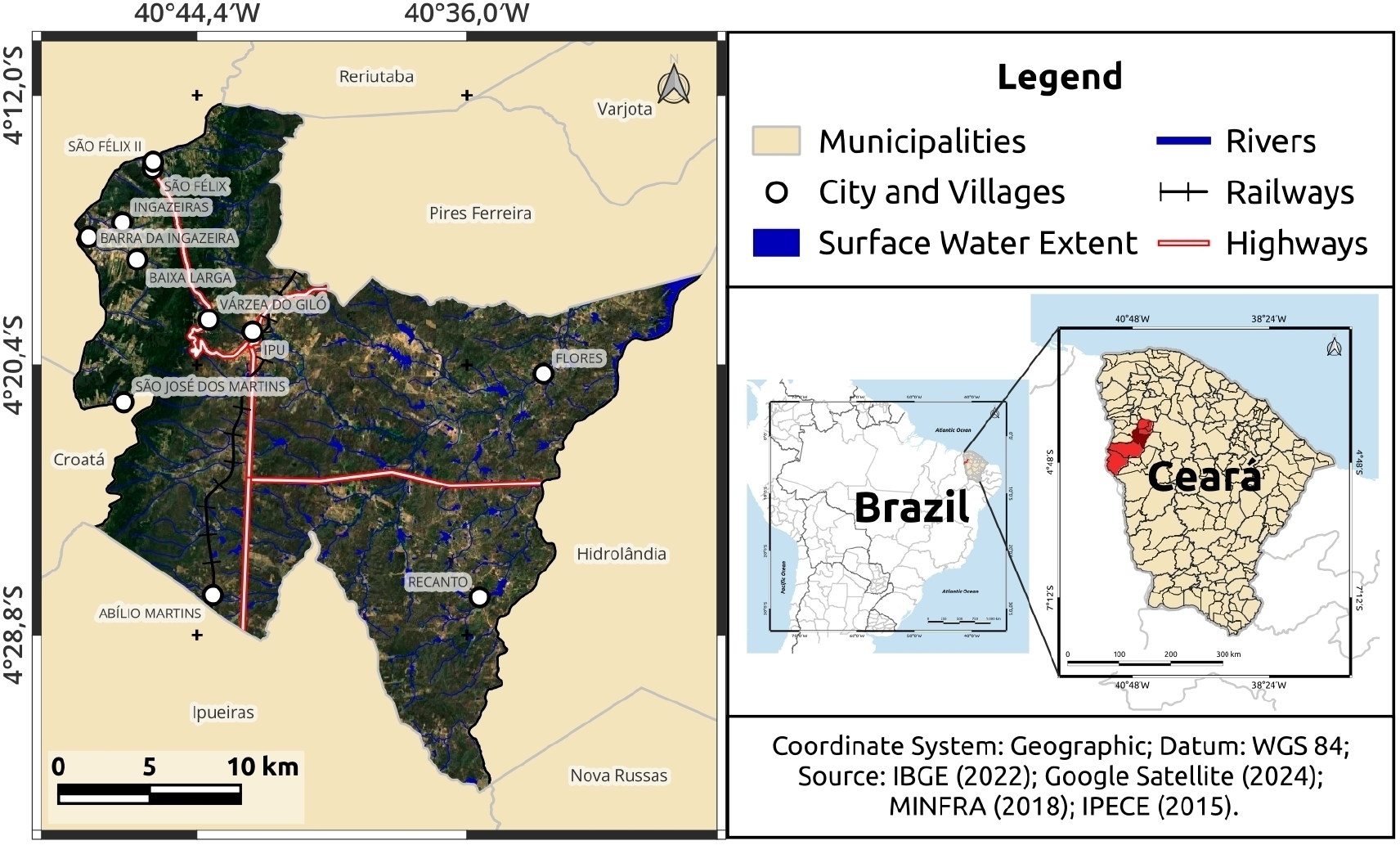
The municipality of Ipu is in the Ceará Northwest (Figure 1), in the Microregion of Ipu and is part of the influence area of the Ubajara National Park [ICMBIO 2017] and recognized by the touristic Ipu Waterfall, area that is part of the “Bica do Ipu” Environmental Protection Area (APA, acronym from brazil portuguese). The municipality comprises an urban center at its headquarters and five residential districts spread over rural areas. More than 46% of the municipality’s formal employees are involved in agriculture activities, responsible for 23.21% of the Gross Value Added (VAB), which mainly produced 4,330 tons of corn, 1,147 tons of beans in 2023 and more than 13,000 of cattle [IPECE 2024].

Figure 1
Ipu Location Map.

De Freitas et al. [De Freitas et al. 2017] delimited Ipu’s environmental systems to be planned based on the concept of systems, geosystems and geoecology [Von Bertalanffy 1975], [Bertrand and Bertrand 2007], [Rodriguez and Silva 2002]. Ipu is composed of Sertaneja Depression, an environment of stable transition and moderate vulnerability, called Sertão, from brazil portuguese. It has a crystalline basement with a preserved and moderately dissected flattened surface, with an altitude of 140 - 290 m (Figure 2). This system could develop extensive cattle, crops, vegetables, mineral extraction, dense surface drainage, and surface water extent. However, this system faces limitations related to soil mechanization, salinization, water irregularity, susceptibility to burning, vegetation with low soil protection capacity, erosion processes, and overall low sustainability.

Figure 2
Ipu’s Elevation and Topographic Profiles.

The Sedimentary Ibiapaba Plateau (SIP) is the second major environmental system, composed of the Ipu, Tianguá and Jaicós Formations, Ipu being the oldest of the three formations of the Serra Grande Group [Claudino-Sales et al. 2020]. Its surface is around 900 m above sea level, recent studies characterized this area as a glint, a large escarpment resulting from differential erosion at the edge of a sedimentary basin where the sedimentary material is more resistant than the underlying or adjacent crystalline material [Goudie 2004]. It presents significant potential, including deep soils, high annual rainfall indices, subsurface water resources, and most importantly, suitability for agriculture. However, it also faces limitations such as soil acidity and low fertility, steep slopes with deforestation on hillsides, and a low potential for surface water availability. The topographic profile A from Figure 2 presents an individual characteristic of this segment, the anaclinal rivers, which due to the process of differentiated erosion run counter to the escarpment forming waterfalls such as Ipu Waterfall [Claudino-Sales et al. 2020], differently of the pattern from SIP represented in the topographic profile B.

Finally, the River Plains environmental system is flat, resulting from the fluvial accumulation and subject to periodic flooding, bordering the river channels and widening in the lower valleys; due to the intermittent regime of the rivers, the fluvial plain occupies a small area, being reversed by riparian forests, especially the presence of carnauba trees. The area has potential deep soils, mineral extraction, water availability, irrigation projects, and agricultural activities. However, it also faces significant limitations such as the constraints of permanent preservation areas, the risk of salinization, and challenges in urban areas during the rainy season, which raise concerns about its long-term sustainability. This characterization is fundamental to understand the geometric features that could influence in some level the SAR images processing in this study.

DATA AND PROCESSING

We used Sentinel-1A level 1 data in Single-Look Complex (SLC) dual-pol (VH, VV) from the Interferometric Wide-swath mode (IW) between 07/2021 and 08/2022, the 2021/22 agricultural year, to generate the classification map (Table 1). SLC is obtained in the slant range, that is, the line-of-sight from the SAR to each reflecting object [ESA 2024]. We used the LULC MapBiomas (collection 9) [MapBiomas 2024] products as reference maps to initially obtain the training samples for the RF model for our classification. This data is produced on a large scale using metrics derived from Landsat images of August, September, and October of each year between 1985 and 2023, using RF to classify Brazil. To be conservative, we selected two years from the MapBiomas to ensure overlap between our study period. We adopted a methodological procedure to support mainly temporary crop monitoring divided into two steps:

i) generating SAR features, and ii) integrating the 35 images into a data cube to verify the effectiveness of the SAR features for the temporary crop.

FEATURE EXTRACTION FROM SAR IMAGES

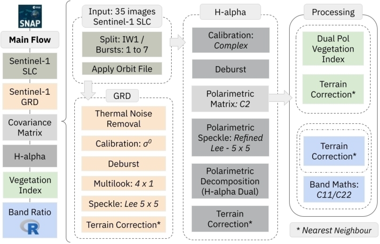
We rigorously processed Sentinel-1 data (Figure 3) to extract the 10 features (Table 2), resulting in over than 230 GB of data. We started with a split, to select the 1 to 7 bursts of interest from the IW1 SAR image in SNAP software [SNAP 2024]. We applied the orbit file to geolocate, removed the thermal noise, calibrated Sigma 0 (σ0) to generate the Ground Range Detected (GRD), and calibrated the complex for the polarimetric process.

Table 2
Features extracted from the Sentinel-1 data.

Features	Method	Feature Parameter	N°
Original	Covar iance matrix	Cll; C12 real; C12 imaginary; C22	4
Polarimetric Decomposition	H/A Alpha	Alpha Angle; H (Entr opy)	2
	DpRVI (Dual Pol Radar- Vegetation Index)		1
SAR Discriminators	GRD (Ground Range Detected)		2
	BR (BandRatio - Cl 1/C22)		1
Total			10

Figure 3
SAR Images Processing.

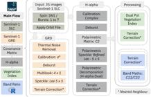
The deburst ensures a continuous and homogeneous image, without burst artifacts. We applied the covariance matrix (C2), utilized to analyze scattering mechanisms and extract key features. For the H-alpha dual polarimetric decomposition (5) we previously applied the Refined Lee (1 look, 5x5). We obtained from the C2 matrix the Dual Pol Radar Vegetation Index (DpRVI) (3) and the ratio bands (C11/C22). We adjust the SAR image geometry for all of the features by applying a geometric correction to ensure an accurate spatial representation of the data from the integration with the SRTM 3Sec digital elevation model using nearest-neighbor nearest-neighbor resampling methods.

SAR DATA CUBE CLASSIFICATION

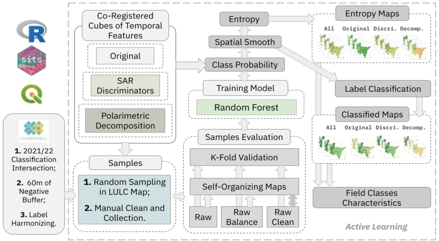
We adopted the active learning approach to perform our analysis. We used the open-source software QGis to clean and increment the training samples and SITS R package [Simões et al. 2021] to create data cubes from the processed Sentinel-1 images, extract time series from the training samples, perform evaluations, classify the images, estimate uncertainties, and validate the classification results (Figure 4). We divided this in three main steps for each and all features: i) samples collection; ii) samples evaluation and training model training; and, iii) classification and evaluation.

Figure 4
SAR Temporal Classification.

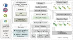
We intersected the 2021 and 2022 LULC reference maps, obtaining classes that remained the same and could represent the same class in our time series. We apply a 60m of negative buffer in each class being conservative to avoid samples in edges. We created a 1km negative buffer of the intersected area from 1 to 7 bursts in the time series and performed the random sample collection. Additionally, we refined the samples by manually cleaning them and adding new collections to improve the classification results. Therefore, it was necessary to harmonize the legend (Table 3). We decided not to use the “Mosaic of Uses” and “Other non Vegetated Areas” classes for the final classification, because they have not performed well in any testing classification, possibly due there are not large areas of them. We balanced the raw sample dataset using the SMOTE algorithm [Chawla et al. 2002].

Table 3
Harmonized classes labels. Note: (^*) Removed classes.

LULC Classes	Harmonized Classes
Forest Formation	Arboreal
Savanna Formation	Shrubby
Pasture	Pasture
Other Temporary Crops	Temporary Crops
Mosaic of Uses*	Mosaic ofUses*
Urban Ar ea	Urban (City and Village)
Other non Vegetated Areas*	Other*
River, Lake and Ocean	Water

We used Self-Organizing Maps (SOM) [Kohonen 1982] using euclidean distance to evaluate the quality of our Raw and Balance samples [Santos et al. 2021]. SOM transforms high-dimensional data into a two-dimensional space, enabling the visualization and identification of fundamental patterns within the data. We conducted sample cleaning in the raw dataset based on the SOM findings, allowing us to identify potential outliers or inconsistencies in the samples. This process aimed to ensure that the samples accurately represented the variability in LULC classes, grouping similar data and spreading differences. Thus, we created a third dataset with clean raw samples.

To evaluate the generalization and robustness of the classification model for Raw, Balance and cleaned samples, we employed the K-Fold cross-validation technique [Stone 1974], widely recognized for its effectiveness in validating predictive models. This technique helps reduce variance associated with partitioning the data into training and testing sets, providing a more reliable estimate of the model’s performance. The classification achieved should be consistent and representative of the entire dataset. However, despite previous knowledge about the study area and some inconsistencies related to the LULC reference, all results were checked to choose our result map.

We used the Random Forest R package [Liaw and Wiener 2002] in SITS to classify the SAR Data Cube. First, we obtained the probabilities of each pixel belonging to a given class. Then, we applied spatial smoothing to consider the continuity between neighboring pixels, assigning weights based on the neighborhood. Finally, we labeled the classes with the highest probability, ensuring a more coherent and spatially consistent classification.

We performed the classification evaluation using specialist knowledge. First, the entropy, which represents the uncertainties associated with the classification, was calculated from the smoothed class probability rasters. We choose the result map that performed better by visual interpretation between entropy maps, optical satellite images, the reference LULC and auxiliary data. It was possible due to the previous knowledge about the study area, associated with photos from the field to reinforce the results found in the chosen map. Building a relation between the field classes characteristics and the map, and how geometric municipality structures may affect the final results.

RESULTS

TRAINING SAMPLES EVALUATION

We extracted 7,655 training samples across the study area. After applying the SMOTE technique to balance our dataset, which we called Balance in Table 4, we obtained 1,468 samples. We also evaluated a third dataset called Clean, which we used 3,279 after the SOM cleaning (Table 4). We manually collected and cleaned some samples due to their lower distribution in the study area. For pasture, we removed points from small fragments. We increment samples from Shrubby and Arboreal and spread their points into big polygons from the LULC reference. For Temporary Crops, we considered them even minor because of their low occurrence.

Table 4
Samples by class for all features.

Classes	Raw	Balance	Clean
Arboreal	1,160	252	559
Shrubby	2,190	252	323
Pastrue	2,200	256	1,584
Temporary Crops	730	256	106
Urban (City and Village)	1,025	256	376
Water	350	196	331
Total	7,655	1,468	3,279

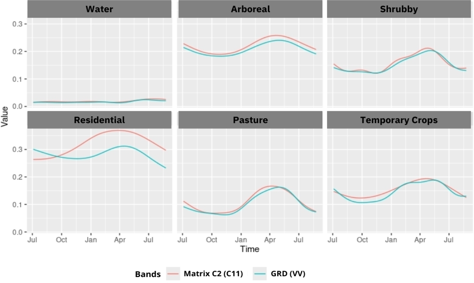
We extracted the temporal patterns for each class using Matrix C2 (C11 parameter) and GRD (VV parameter) (Figure 5). We chose these features because of their relation and similar interval values. The water pattern had lower values until April 2022 and presented a modest increase in May 2022, corresponding to the end of the rainy period in Caatinga. For Arboreal, we identified a regular decrease in values during July and December 2021, followed by an increase reaching their maximum between April and May 2022.

Figure 5
Balance Samples Patterns.

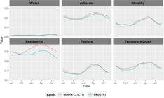
Despite the modestly more significant values for the Shrubby patterns, Temporary Crops present similar values and behavior, presenting short increasing and decreasing values that oppose the main patterns for classes in Caatinga. However, in Temporary Crops this behaviour represents two cycles in six months, starting in January from VV. Urban (City and Village) presents the highest values for the features for almost the entire year. Pasture significantly differs in value between the dry and rainy seasons and reaches minor values between vegetation classes.

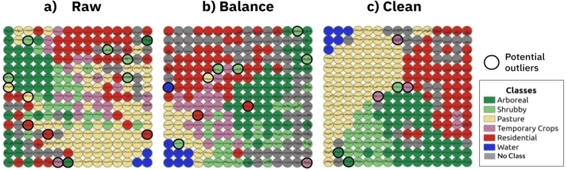
SOM effectively identified confusion between some classes across the time series. While the patterns across all features are consistent, the behavior within each neuron for specific features varies. We chose to show the SOM map based on All Feature samples because it produces the more homogeneous groups. Figure 6 presents the SOM map (15 × 15) for temporal patterns derived from the Dual-Pol Vegetation Index feature, as it exhibits variations over time that are more perceptible to human interpretation.

Figure 6
Dual Pol Vegetation Index feature Som Map (All Features).

We identified 13 potential outliers for Raw samples, 10 for Balance samples, and 6 for Clean samples. We considered the outlier neurons according to three premises: neurons classified differently from the neighboring majority class, more than three neurons away, and groups with at least three neurons. The SOM analysis using the mixture matrix revealed substantial class mixing, with confusion levels exceeding 20% for Raw samples, reducing to 15% for Balance samples, and falling below 10% for Clean samples (Supplementary Material Figure 1).

The Balance sample achieved better grouping for Temporary Crops, with only one outlier (Figure 6b). Otherwise, the Raw sample (Figure 6a) exhibited more dispersed neurons, with connections forming diagonal patterns or small groups of two neurons, despite having just one Temporary Crops outlier. For Clean samples (Figure 6c), there were three Temporary Crops outliers, but only two neurons grouped. We got empty neurons (No Class) in the three evaluated datasets; Balance samples had the highest count (57), followed by Clean (28) and Raw (22). Despite its limitations in grouping Temporary Crops and being second in terms of No Class neurons, the Clean sample visually demonstrated improved grouping for the other classes (Figure 6c).

After data cleaning, the K-fold results provided a comprehensive evaluation of model generalization and robustness across different datasets and feature sets. The All Features configuration demonstrated accuracy values ranging from 75.9% to 79.7% in the Raw and Balance dataset and achieved 97.3% in the Clean dataset, indicating a significant improvement due to data cleaning. Similar trends were observed in other feature sets, with Balance and Clean accuracies consistently outperforming Raw samples (Table 5).

Table 5
K-fold Overall Accuracy (95% confidence).

Features	Raw (%)	Balance (%)	Clean (%)
All Features	75.9	79.7	97.3
Original	56.2	59.5	94.5
Polarimetric Decomposition	75.1	62.2	97.8
SAR Discriminators	75.5	83.1	97.8

The Original feature set exhibited the lowest performance among the configurations, achieving accuracies of 56.2% in Raw and 59.5% in Balance but improving substantially to 94.5% in Clean. On the other hand, SAR Discriminators achieved the best results for Balance (83.1%) and Clean (97.8%), outperforming all other feature sets in Balance and Clean. For Raw datasets, accuracies were comparable across All Features, Polarimetric Decomposition, and SAR Discriminators, all hovering around 75%.

CLASSIFICATION MAPS

We produced 12 classified maps (Supplementary Material Figure 2). Water was well classified in all maps, followed by the Urban (City and Village), mainly limited in the Original classification (Supplementary Material Figure 2 B, F, and J) and over-classified in the Polarimetric Decomposition (Supplementary Material Figure 2 C, G, and K). Shrubby was partially hidden in Original and Polarimetric Decomposition in Raw and Clean, despite appearing better for the Balance (Supplementary Material Figure 2 E, F, G, and H). SAR discriminators and all features look similar, but the classification of all features from balance samples especially adheres to the visual and previous knowledge about municipality dynamics (Supplementary Material Figure 2 E).

We selected the classification of All Features from Balance samples as our primary product by visual analysis (Figure 7). The previous knowledge about the study area permitted us to make this decision due to the distribution identified for Temporary Crops and Arboreal classes within the Sertão region, which cover 28.1 km² and 156 km² of the study area, respectively (Figure 7). The Shrubby class encompassed the most significant area at 303.5 km² and dominated the municipality with 47.3%, mainly distributed and being the landscape matrix in the Sertão.

Figure 7
All Features from Balance Samples.

The Arboreal class is the second largest area, representing 24.3% of the study area, and is the landscape matrix in the mountainous region. It is followed by the Pasture class, with 21.2%, mainly spread in Sertão and bordering the Temporary Crops and the highway in the mountainous region (Figure 1). The urban (City and Village) and Water classes align with the municipal districts and rivers (Figure 1), occupying 7.4 km² and 10.4 km², respectively.

FIELD CLASSES CHARACTERISTICS

We identified the relationship between the classification and the field class characteristics from local observations and prior knowledge about the study area. In the first observation, we found a similar pattern from the LULC reference (Figure 8.1) despite the higher uncertainty values between 800 and 1000. Where we identified the same classes but in different concentrations, with more areas of Temporary Crops. The Arboreal class area achieves lower uncertainty values and changes the landscape matrix previously classified as Shrubby by the LULC reference in the mountainous region. In Optical Image, we have farms, rivers, and urban areas mapped by federal and state agencies, confirming our results.

Figure 8
Visual Interpretation.

Figure 9
New areas identified (2024).

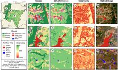
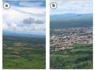
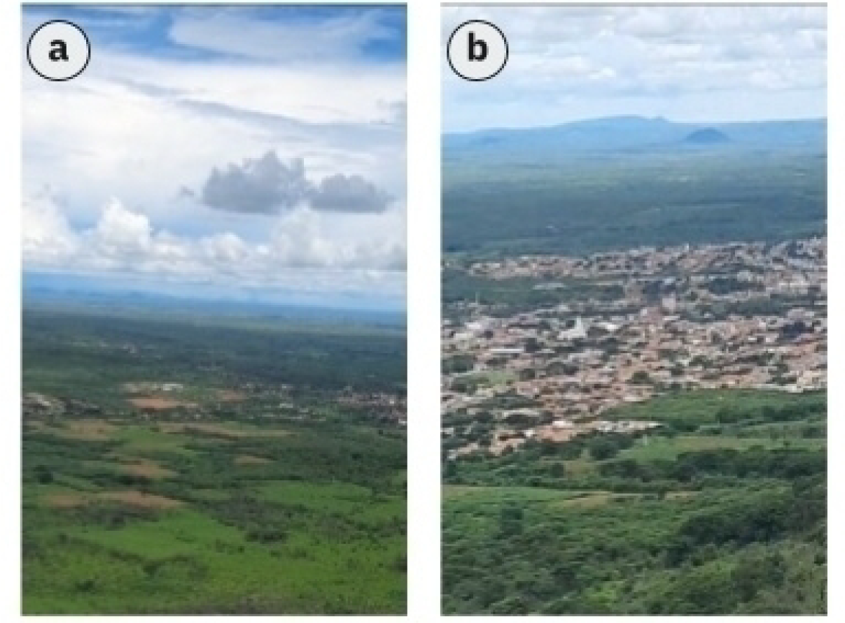
In the second observation, we identified new areas of Temporary Crops and more Arboreal and Pasture classes (Figure 8.2) next to the Urban (City and Village) area, which we confirmed from field observation (Figure 10). We registered it from the mountainous region with a view of the seat of the municipality, from northwest to southeast. The uncertainty reaches significant levels in the escarpment area, for the Arboreal class achieved middle levels, between 500 and 600, and low levels for the Pasture and Urban (City and Village) classes, between 300 and 400.

Figure 10
Corn Dynamic in Sertão (2024).

In the third (Figure 8.3), we identified Arboreal and Temporary Crops in the middle of Sertão, where the LULC reference classified as Shrubby, Pasture and Water classes. The Arboreal class was distributed along the river course, as presented in Optical Image, with uncertainty values between 600 and 700. The Temporary Crops areas are small, about 1 ha, and next to these areas. Pasture reaches low-uncertainty, between 300 and 400, but the values are even lower to Water, between 10 and 100.

DISCUSSION

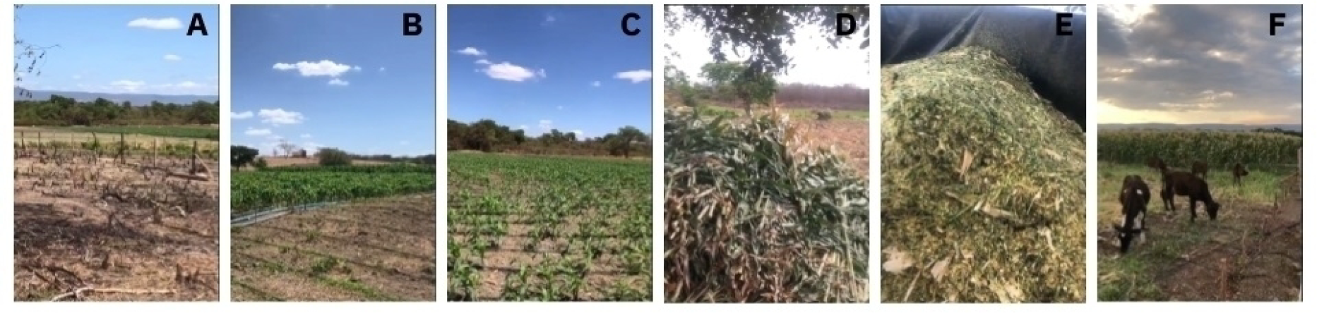
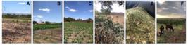
Using Machine Learning methods, specifically, Random Forest (RF), combined with SAR image time series properly processed to perform a Land Use and Land Cover classification, can result in accurate maps with strong generalization capabilities. A key factor in this approach is the need for heterogeneous training samples that exhibit a high degree of separability from other classes, reducing bias. This was guaranteed in the Active Learning approach adopted during the execution of the classification rounds [Crawford et al. 2013]. The pattern curves found for the training samples reflected the expected characteristics of each class over time, suggesting that the training samples adequately captured the spectral variations of the classes. In our results we identified the temporal patterns of the samples from the Temporary Crops (Figure 5), which we could identify in Sertão, far from the mountains. We confirm this when we analyze Figure 11: i) the corn dynamic involves deforestation (a), irrigation (b), crop development (c), harvest (d), processing (e), cattle before new planting (f); ii) following the sample pattern.

Figure 11
Water Seasonality (2024).

The choice of a 15 × 15 SOM was driven by the need to adequately distribute the higher number of neurons required for the Raw samples (7,655), which also supports the Balance (1,468) and Clean (3,279) samples without compromising interpretative value. This ensures the map preserves topological relationships across datasets with varying sizes, as SOM naturally adapts to the data density in different map regions. The presence of No Class neurons, particularly in the Balance sample, reflects regions of the feature space not represented by the dataset. Using a fixed grid size across datasets with varying densities is a natural outcome.

We had some potential outliers in SOM, this suggests that the classes share similar characteristics. The neuron arrangement highlights the impact of this confusion on class separability over the years, that are not necessarily the result of mislabeled samples, they can represent samples that have different patterns of land use and land cover classes in space or time, or samples that are not separable using time series or metrics extracted from them. Overall, the Dual Pol Vegetation Index feature stands out for its sensitivity to temporal variations, which aligns with the goal of using SOM for temporal pattern analysis. Future work could explore adaptive SOM grid sizes or weighted feature contributions to further optimize the map for datasets with high variability in sample sizes.

Reducing outliers and confusion levels from Raw to Balance and Clean samples demonstrates the importance of preprocessing steps, such as balance and clean, to refine class separability. However, the better grouping of Temporary Crops in the Balance sample emphasizes that reducing sample size and class imbalance can enhance cluster formation for minority classes without heavily impacting the overall map structure.

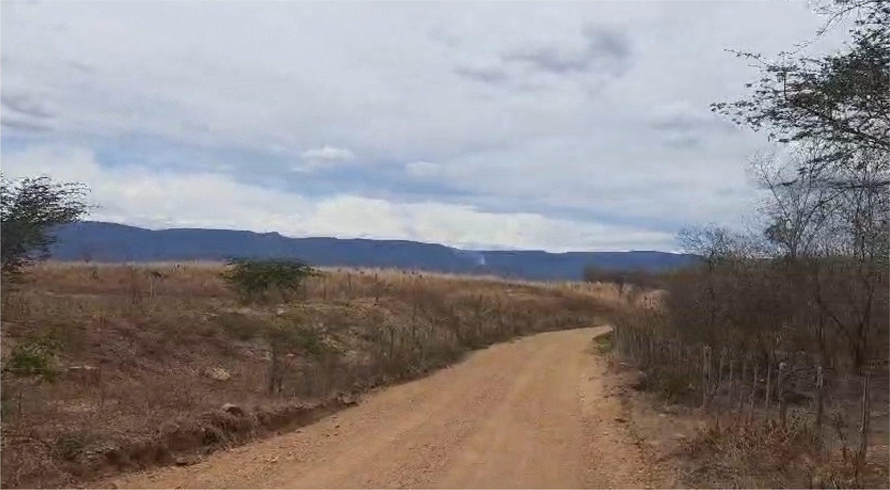
Time series approach improves our results by providing the temporal behavior of our classes, considering the seasonality of the Caatinga [Brito et al. 2023], differently from the LULC reference [MapBiomas 2024]. We evidence it by Figure 11, where in less than 6 months the surface water extent can vary significantly. The temporal pattern from Dual Pol Vegetation Index presents a peak of vegetation during the rainy season, as can be seen in the 2024 image (Figure 11 A and C). Additionally, to classify a small area, as a municipal scale, demands a large volume of data processing and computational power, to perform this time series classification. Known effects in SAR images from geometric characteristics such as shadow, ramp shortening, layover, may contribute to some uncertainty in classification [Hansen 2001]. Once the municipality had an abrupt difference in altitude between the Sertão and the mountainous areas (Figure 12).

Figure 12
Geometric Characteristics (2024).

CONCLUSION

This study demonstrates the feasibility and relevance of using Sentinel-1 time series data combined with data cube methodologies to monitor and classify agricultural activities in the municipality of Ipu-CE. We achieved accurate Land Use and Land Cover classifications with significant generalization capabilities by leveraging Random Forest (RF) machine learning methods and adopting an Active Learning approach to enhance training sample heterogeneity.

The temporal patterns identified in the dataset highlighted the dynamic nature of agricultural cycles, particularly in corn cultivation, as influenced by deforestation, irrigation, crop development, harvest, and post-harvest land use. These findings underscore the importance of time series analysis in capturing the seasonal behavior specific to the Caatinga biome, which are less apparent in LULC reference.

The challenges associated with processing large datasets and addressing SAR- specific geometric distortions - such as shadowing, ramp shortening, and relief inversion - were evident, especially given the sharp altitudinal gradients within the study area. Overall, this study’s results contribute to the advancement of agricultural monitoring in semiarid regions by providing high-resolution, temporally informed classifications. The insights generated can support the development of public policies promoting sustainable agricultural practices while improving resilience to environmental variability.

Future work may focus on scaling these methodologies to larger regions and integrating additional datasets to enhance classification accuracy and applicability further.

NOTES

• (1)
  A Scopus search on December 13th 2024, of “SAR” AND “Caatinga” OR “Datacube” returned 14 articles

ACKNOWLEDGMENT

My father MP and my friend EL for the photos and information of the local characterization. This study was financed in part by the Coordenação de Aperfeiçoamento de Pessoal de Nível Superior Brasil (CAPES) - Finance Code 001.

REFERENCES

• Adami, M., Rudorff, B. F. T., Freitas, R. M., Aguiar, D. A., Sugawara, L. M., and Mello, M. P. (2012). Remote sensing time series to evaluate direct land use change of recent expanded sugarcane crop in brazil. Sustainability, 4(4):574-585.
• Barra, A., Monserrat, O., Mazzanti, P., Esposito, C., Crosetto, M., and Scarascia Mugnozza, G. (2016). First insights on the potential of sentinel-1 for landslides detection. Geomatics, Natural Hazards and Risk, 7(6):1874-1883.
• Bertrand, G. and Bertrand, C. (2007). Uma geografia transversal e de travessias: o meio ambiente através dos territórios e das temporalidades. Maringá: Massoni, 360.
• Brazil (2024). Institutes the national policy for the recovery of the caatinga vegetation. Pending approval in the Chamber of Deputies after Senate approval.
• Brito, P., Chaves, M., Carvalho, H., Souza, F., Silva, B., Ferreira, K., Santos, R., and de Queiroz, G. R. (2023). Uso de séries temporais para classificação de uso e cobertura da terra em Petrolina, Pernambuco.
• Claudino-Sales, V., Lima, E., Diniz, S., and Cunha, F. (2020). Megageomorfologia do planalto da ibiapaba, estado do Ceará: uma introdução. William Morris Davis-Revista de Geomorfologia, 1(1):186-209.
• Cloude, S. R. and Pottier, E. (1996). A review of target decomposition theorems in radar polarimetry. IEEE transactions on geoscience and remote sensing, 34(2):498-518.
• Crawford, M. M., Tuia, D. and Yang, H. L. (2013) “Active Learning: Any Value for Classification of Remotely Sensed Data?” Proceedings of the IEEE, vol. 101, no. 3, pp. 593-608, doi: 10.1109/JPROC.2012.2231951.
  » https://doi.org/10.1109/JPROC.2012.2231951.
• De Freitas, A. L. R., Rabelo, F. D. B., da Silva, E. V., and Lima, E. C. (2017). Técnicas de geoprocessamento para delimitação de sistemas físico-naturais e ações de planejamento: o caso do município de Ipu-ce. Os Desafios da Geografia Física na Fronteira do Conhecimento, 1:5709-5714.
• Diniz, J. M. F. d. S., Gama, F. F., and Adami, M. (2022). Evaluation of polarimetry and interferometry of sentinel-1a sar data for land use and land cover of the brazilian amazon region. Geocarto International, 37(5):1482-1500.
• Doblas, J., Shimabukuro, Y., Sant’Anna, S., Carneiro, A., Aragão, L., and Almeida, C. (2020). Optimizing near real-time detection of deforestation on tropical rainforests using sentinel-1 data. Remote Sensing, 12(23):3922.
• ESA (2024). S1 processing. European Space Agency (ESA). Accessed on 14 December 2024.
• European Space Agency (2021-2022). Copernicus sentinel-1 data [2021, 2022]. Accessed via the Copernicus Open Access Hub.
• European Space Agency (2024). Sentinel-1 SAR User Guide. Online; accessed 14 May 2024.
• European Space Agency (ESA) (2024). Sentinel-1 mission overview. Accessed: 2024-12-13.
• Ferreira, K. R., Queiroz, G. R., Vinhas, L., Marujo, R. F., Simões, R. E., Picoli, M. C., Camara, G., Cartaxo, R., Gomes, V. C., Santos, L. A., et al. (2020). Earth observation data cubes for Brazil: Requirements, methodology and products. Remote Sensing, 12(24):4033.
• Gama, F. F., Wiederkehr, N. C., and da Conceição Bispo, P. (2022). Removal of ionospheric effects from sigma naught images of the alos/palsar-2 satellite. Remote Sensing, 14(4):962.
• Ganem, K. A., Dutra, A. C., de Oliveira, M. T., de Freitas, R. M., Grecchi, R. C., da Silva Pinto Vieira, R. M., Arai, E., Silva, F. B., Sampaio, C. B. V., Duarte, V., and Shimabukuro, Y. E. (2020). Mapping caatinga vegetation using optical earth observation data: Opportunities and challenges. Revista Brasileira de Cartografia, 72(50th).
• Goudie, A. (2004). Encyclopedia of geomorphology. Routledge.
• Hanssen, R. F. (2001). Radar interferometry: data interpretation and error analysis, volume 2. Springer Science & Business Media.
• ICMBIO (2017). Plano de Manejo: Encarte 4 - Contexto Regional. http://www.icmbio.gov.br/parnaubajara/planos-de-manejo Accessed: 26 nov. 2024.
  » http://www.icmbio.gov.br/parnaubajara/planos-de-manejo
• IPECE (2024). IPECE DATA - Sistema de Informações Geossocioeconômicas do Ceará. http://ipecedata.ipece.ce.gov.br/ipece-data-web/module/perfil-municipal.xhtml Accessed: 26 nov. 2024.
  » http://ipecedata.ipece.ce.gov.br/ipece-data-web/module/perfil-municipal.xhtml
• Kasischke, E. S., Melack, J. M., and Dobson, M. C. (1997). The use of imaging radars for ecological applications-a review. Remote sensing of environment, 59(2):141-156.
• Kohonen, T. (1982). Self-organized formation of topologically correct feature maps. Biological cybernetics, 43(1):59-69.
• Le Toan, T. and Floury, N. (1998). On the retrieval of forest biomass from sar data. EUROPEAN SPACE AGENCY-PUBLICATIONS-ESA SP, 441:213-214.
• Lee, J.-S., Jurkevich, L., Dewaele, P., Wambacq, P., and Oosterlinck, A. (1994). Speckle filtering of synthetic aperture radar images: A review. Remote sensing reviews, 8(4):313-340.
• Liao, H., Wdowinski, S., and Li, S. (2020). Regional-scale hydrological monitoring of wetlands with sentinel-1 insar observations: Case study of the south florida everglades. Remote Sensing of Environment, 251:112051.
• Liaw, A. and Wiener, M. (2002). Classification and regression by randomforest. R News, 2(3):18-22.
• López Martinez, C. (2003). Multidimensional speckle noise. Modelling and filtering related to sar data. Universitat Politècnica de Catalunya.
• N. V. Chawla, K. W. Bowyer, L. O. Hall, and W. P. Kegelmeyer, “SMOTE: Synthetic minority over-sampling technique,” Journal of Artificial Intelligence Research, vol. 16, no. 1, pp. 321-357, 2002.
• MapBiomas (2024). ATBD - ENTENDA CADA ETAPA. Online; accessed 25 May 2024.
• Markham, C. G. (1967). Climatological aspects of drought in northeastern Brazil. University of California, Berkeley.
• Moreira, A., Prats-Iraola, P., Younis, M., Krieger, G., Hajnsek, I., and Papathanassiou, K. P. (2013). A tutorial on synthetic aperture radar. IEEE Geoscience and remote sensing magazine, 1(1):6-43.
• Paradella, W. R., Knust, S. S. A., Dos Santos, A. R., Silva, A., Rabelo, T. N., and Oliveira, C. (2009). Influence of macroscale and microscale surface roughness on multibeam radarsat-1 data: implications for geological mapping in the curaçá valley (Brazil). Photo interprétation (Paris), 45(2).
• Pelletier, C., et al. (2016). Assessing the robustness of Random Forests to map land cover with high resolution satellite image time series over large areas. Remote Sensing of Environment, 187:156-168.
• Pelletier, C., Webb, G. I., and Petitjean, F. (2019). Temporal convolutional neural network for the classification of satellite image time series. Remote Sensing, 11(5):523.
• Picoli, M. C. A., Câmara, G., Sanches, I., Simões, R., Carvalho, A., Maciel, A., Coutinho, A., Esquerdo, J., Antunes, J., Begotti, R. A., et al. (2018). Big earth observation time series analysis for monitoring brazilian agriculture. ISPRS journal of photogrammetry and remote sensing, 145:328-339.
• Rodriguez, J. M. M. and da Silva, E. V. (2002). A classificação das paisagens a partir de uma visão geossistêmica. Mercator, 1(1).
• Sano, E. E., Bolfe, É . L., Parreiras, T. C., Bettiol, G. M., Vicente, L. E., Sanches, I. D. A., and Victoria, D. d. C. (2023). Estimating double cropping plantations in the brazilian cerrado through planetscope monthly mosaics. Land, 12(3):581.
• Sano, E. E., Ferreira, L., Asner, G., and Steinke, E. (2007). Spatial and temporal probabilities of obtaining cloud-free landsat images over the brazilian tropical savanna. International Journal of Remote Sensing, 28(12):2739-2752.
• Santos, L. A., Ferreira, K. R., Camara, G., Picoli, M. C., & Simoes, R. E. (2021). Quality control and class noise reduction of satellite image time series. ISPRS Journal of Photogrammetry and Remote Sensing, 177:75-88.
• Simões, R., Camara, G., Queiroz, G., Souza, F., Andrade, P. R., Santos, L., Carvalho, A., and Ferreira, K. (2021). Satellite image time series analysis for big earth observation data. Remote Sensing, 13(13):2428.
• Simões, R., Picoli, M. C., Camara, G., Maciel, A., Santos, L., Andrade, P. R., Sánchez, A., Ferreira, K., and Carvalho, A. (2020). Land use and cover maps for Mato Grosso state in brazil from 2001 to 2017. Scientific Data, 7(1):34.
• SNAP (2024). Sentinel Application Platform - SNAP 10.0.0. https://step.esa.int/main/download/snap-download/ Online; accessed 25 May 2024.
  » https://step.esa.int/main/download/snap-download
• Stone, M. (1974). Cross-validatory choice and assessment of statistical predictions. Journal of the royal statistical society: Series B (Methodological), 36(2):111-133.
• Tomppo, E., Antropov, O., and Praks, J. (2019). Cropland classification using sentinel-1 time series: Methodological performance and prediction uncertainty assessment. Remote Sensing, 11(21):2480.
• Truckenbrodt, J., Freemantle, T., Williams, C., Jones, T., Small, D., Dubois, C., Thiel, C., Rossi, C., Syriou, A., and Giuliani, G. (2019). Towards sentinel-1 sar analysis-ready data: A best practices assessment on preparing backscatter data for the cube. Data, 4(3):93.
• Ulaby, F. T., Moore, R. K., and Fung, A. K. (1982). Microwave remote sensing: Active and passive. volume 2-radar remote sensing and surface scattering and emission theory.
• Von Bertalanffy, L. (1975). Teoria geral dos sistemas. Vozes Petrópolis.

• Editors in Charge
  Alexandra Maria Oliveira
  Alexandre Queiroz Pereira

Publication Dates

• Publication in this collection
  30 June 2025
• Date of issue
  2025

History

• Received
  20 Jan 2024
• Accepted
  30 Jan 2024
• Published
  10 Mar 2025