An Exact Geometrically Nonlinear 3D Truss Finite Element with Variable Axial Rigidity Based on Positional Formulation

Abstract

This paper introduces an exact geometrically nonlinear 3D truss finite element based on the positional formulation, capable of accounting for arbitrarily varying axial rigidity along the element’s length. The proposed formulation accurately captures large-displacement behavior using a single element per member, without requiring mesh refinement. A key advantage is the elimination of local-to-global coordinate transformations, thereby reducing computational cost. The formulation derives the axial flexibility using the flexibility method and the principle of virtual forces, avoiding the need for exact shape functions. Numerical examples, including 2D and 3D trusses with polynomial axial rigidity variations, show perfect agreement with analytical solutions in terms of nodal displacements, nodal positions, axial forces, and limit loads. The method also exhibits faster convergence compared to existing approaches, confirming its accuracy, robustness, and efficiency as a powerful technique for geometrically nonlinear analysis of truss structures with arbitrarily varying axial rigidity.

Keywords:
Geometric nonlinearity; Positional formulation; Variable axial rigidity; 3D truss finite element

Graphical Abstract

1 INTRODUCTION

Truss structures are extensively employed in a wide range of engineering applications, including long-span bridges, roofs, walkways, transmission towers, cranes, and aerospace structures. Their popularity stems from an optimal combination of low self-weight, high load-capacity, and structural efficiency, making them ideal for structures where span and weight are critical.

The structural response of trusses under service loads often involves significant displacements, necessitating numerical models that can accurately capture geometric nonlinear effects. Furthermore, the presence of nonprismatic members or those with functionally graded material properties requires models that can account for variable axial rigidity along the element's length. Ignoring these aspects can lead to potentially unsafe, inaccurate predictions of displacements, internal forces, and ultimate load-carrying capacity.

Various formulations based on the Finite Element Method (FEM) have been established to investigate geometric nonlinearity in structural mechanics. The Lagrangian description tracks particle motion relative to a reference configuration. It is implemented in two primary frameworks: the Total Lagrangian (TL) formulation, which references all kinematic and static quantities to the fixed initial configuration, and the Updated Lagrangian (UL) formulation, which continually updates the reference state to the last calculated configuration (Crisfield, 1991; Bathe, 2006; Reddy, 2015). An alternative approach, the corotational (CR) formulation (Crisfield, 1991), effectively separates the rigid-body motions from the local deformations by employing a reference frame that translates and rotates with the element. Closely related to these, the formulation for flexible multibody system dynamics, as extensively detailed by Shabana (2020), provides a comprehensive framework for handling large rotations and displacements in interconnected systems, often employing a TL description with a material (body-attached) coordinate system. In contrast, the positional formulation (Coda and Greco, 2004; Greco and Coda, 2006) offers a distinct methodology by directly describing the equilibrium of the deformed structure in terms of absolute nodal positions within the global coordinate system. This approach inherently eliminates the need for local-to-global coordinate transformations, thereby reducing computational overhead and simplifying the numerical implementation.

A substantial body of literature exists on the geometrically nonlinear analysis of trusses with constant axial rigidity. Seminal and contemporary works in this area include studies by Greco and Venturini (2006), Greco et al. (2006, 2012), Saffari et al. (2008), Greco and Ferreira (2009), Thai and Kim (2009), Souza et al. (2022), and more recent contributions such as Greco and Peixoto (2021) and Silva et al. (2024). These studies have leveraged various strain measures and solution algorithms to trace the nonlinear equilibrium path of truss structures. For the specific case of trusses with polynomially varying axial rigidity, the studies by Kutis and Murín (2005) and Duris and Murín (2007) are noteworthy; they employed the TL formulation with exact shape functions to accurately compute the full nonlinear tangent stiffness matrix. Recent advancements continue to explore these themes, with works investigating the application of advanced materials, such as composites and functionally graded materials, in structural elements (Khan et al., 2016; Rabelo et al., 2018).

Despite these advances, a significant limitation persists in commercial finite element software (e.g., ANSYS®, SAP2000®, ABAQUS®), which typically lacks dedicated elements to precisely capture continuous axial rigidity variation. Consequently, analysts must resort to mesh refinement or the use of multiple standard elements per structural member to approximate the rigidity variation, leading to increased computational cost and, particularly, potential convergence issues in geometrically nonlinear analysis. Moreover, the reliance on linear shape functions for such members yields approximate solutions, further necessitating a finer discretization to achieve acceptable accuracy.

To bridge this gap, this paper presents the formulation and numerical validation of an exact geometrically nonlinear 3D truss finite element based on the positional formulation, capable of modeling arbitrarily variable axial rigidity along its length. The proposed approach accurately captures large-displacement behavior using only a single element per member, irrespective of the rigidity variation. Its principal computational advantage lies in the elimination of local-to-global transformations. The formulation derives the axial flexibility using the flexibility method and the Principle of Virtual Forces (PVF), circumventing the need for exact shape functions. The numerical results demonstrate perfect agreement with analytical benchmarks, confirming the element's computational efficiency, accuracy, and robustness.

2 FINITE ELEMENT FORMULATION

When an elastic structure is subjected to conservative external forces, it stores energy as strain energy, and the forces perform work on the structure. The equilibrium configuration of the structure can be described by the total potential energy functional, denoted by $\text{Π}$, which is defined as the difference between the strain energy U and the potential energy of the external forces P. Mathematically, this is expressed as:

$$$$ $\Pi =U-P$ (1)

However, the strain energy can be expressed as the integral of the strain energy density $u$ over the initial volume of the body $V$as follows:

$$$$ $$U={\displaystyle \underset{V}{\int }udV}={\displaystyle \underset{V}{\int }{\displaystyle \underset{\epsilon }{\int }\sigma d\epsilon dV}}={\displaystyle \underset{V}{\int }{\displaystyle \underset{\epsilon }{\int }E\epsilon d\epsilon dV}}=\frac{1}{2}{\displaystyle \underset{V}{\int }E{\epsilon }^{2}dV}$$ (2)

In Eq. (2), $\sigma$ is the normal stress, which according to Hooke’s law is given by $\sigma =E\epsilon$, where $E$ is the Young’s modulus and $\epsilon$ is the normal strain. The potential energy of the external forces can be expressed as:

$$$$ $P={\displaystyle \sum F\chi }$ (3)

where $\chi$ is the nodal position of the element, in the deformed configuration, in the direction of the applied force $F$.

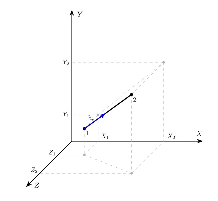
Figure 1 illustrates a truss element oriented in space with respect to a global Cartesian coordinate system. The nodal positions in the deformed configuration are $X_1$, $Y_1$, $Z_1$, $X_2$, $Y_2$, and $Z_2$, where the subscript identifies the node of the element. In the undeformed configuration, these nodal positions are denoted by the superscript (⁰).

Figure 1
3D truss finite element.

The axial force in the element in an arbitrary configuration, assuming the engineering (linear) strain measure, can be expressed in terms of the axial stiffness coefficient $k_{11}$ and the change in length $l-l_0$ as:

$$$$ $N=k_{11}(l-l_0)$ (4)

where

$k_{11}=\frac{1}{f_{11}}$

$$l=\sqrt{{(X_2-X_1)}^2+{(Y_2-Y_1)}^2+{(Z_2-Z_1)}^2}$$

$$l_0=\sqrt{{(X_2^0-X_1^0)}^2+{(Y_2^0-Y_1^0)}^2+{(Z_2^0-Z_1^0)}^2}$$

Although the positional formulation employs exclusively global coordinates to describe equilibrium, the spatial variation of axial rigidity $EA\left(\xi \right)$ is inherently defined along the local axis of the element. The integral defining the axial flexibility coefficient $f_{11}$ in Eq. (5) is evaluated along the dimensionless coordinate $\xi \in \left[\mathrm{0,}1\right]$, which parameterizes the position along the initial element length. Thus, the axial force $N$ is obtained directly from the global nodal positions using Eq. (4). Consequently, the total potential energy functional, the residual force vector, and the Hessian matrix are expressed entirely in the global coordinate system, ensuring consistency and eliminating the computational overhead associated with local axis rotations.

It is worth emphasizing that $N$ in Eq. (4) is invariant under rigid body motion, where $N>0$ denotes tension in the element. The axial flexibility coefficient $f_{11}$ is derived using the flexibility method and the PVF. In the local coordinate system, the truss element has only two degrees of freedom, one at each node. Thus, $f_{11}$ corresponds to the axial displacement at node 1 when a compressive unit axial force is applied at the same node, while node 2 is fixed. Considering equilibrium, this results in a constant axial force of $N=-1$. Therefore, applying the unit load method from the PVF, and considering a dimensionless coordinate $\xi$ along the initial length, yields:

$$$$ $$f_{11}=l_0{\displaystyle {\int }_0^1\frac{d\xi }{EA(\xi )}}$$ (5)

where $EA\left(\xi \right)$ is the continuously varying axial rigidity.

Alternatively, the axial force can be calculated by integrating the normal stress over the initial cross-sectional area $A$ as follows:

$$$$ $$N={\displaystyle \underset{A}{\int }\sigma dA}={\displaystyle \underset{A}{\int }E\epsilon dA}=EA(\xi )\epsilon$$ (6)

Once the axial force is already defined in Eq. (4), the relation in Eq. (6) is used to obtain the normal strain $\epsilon$. Then, the strain energy is obtained by substituting Eq. (4) into Eq. (6) and subsequently substituting the resulting equation into Eq. (2). For convenience, Eq. (2) is rewritten in terms of a double integral over the initial cross-sectional area and along the initial length. Thus, one obtains:

$$$$ $$U=\frac{1}{2}{l}_0{\displaystyle {\int }_0^1{\displaystyle \underset{A}{\int }E{\epsilon }^{2}dAd\xi }}=\frac{1}{2}{l}_0{\displaystyle {\int }_0^{1}EA(\xi ){\epsilon }^{2}d\xi }=\frac{1}{2}{k}_{11}{(l-l_0)}^2$$ (7)

From Eqs. (1), (3), and (7), the total potential energy functional can be expressed in terms of the positions and applied forces, given by:

$$$$ $$\Pi =\frac{1}{2}{k}_{11}{(l-l_0)}^2-F_{X1}{X}_1-F_{Y1}{Y}_1-F_{Z1}{Z}_1-F_{X2}{X}_2-F_{Y2}{Y}_2-F_{Z2}{Z}_2$$ (8)

According to the principle of stationary total potential energy, the equilibrium configuration of an elastic structure corresponds to a stationary point of the total potential energy functional. Mathematically, this can be expressed as:

$$$$ $\frac{\partial \Pi }{\partial {\chi }_i}=g_i=\frac{\partial U}{\partial {\chi }_i}-F_i=f_i-F_i=0$ (9)

where ${\chi }_i$ is a generalized parameter in which the subscript $i$ denotes the degree of freedom corresponding to the nodal position along the global axes, as follows: $\left(\mathrm{1,}\mathrm{2,}\mathrm{3,}\mathrm{4,}\mathrm{5,}6\right)=\left(X_1,Y_1,Z_1,X_2,Y_2,Z_2\right)$. However, Eq. (9) can be rewritten in vector form as:

$$$$ $g(\chi )=f(\chi )-F=0$ (10)

where $g\left(\chi \right)$, $f\left(\chi \right)$, and $F$ are vectors representing the residual force, the internal force, and the external force, respectively.

To solve Eq. (10), the Newton–Raphson method is employed, in which $g\left(\chi \right)$ is expressed by a first-order Taylor series expansion about ${\chi }_0$. Thus, the following expression is obtained:

$$$$ $g(\chi )\approx g({\chi }_0)+H({\chi }_0)\Delta \chi =0$ (11)

where $\chi$ and ${\chi }_0$ are vectors representing the current and initial positions, respectively. Hence, Eq. (11) can be rewritten in a simplified form as:

$$$$ $H({\chi }_0)\Delta \chi =-g({\chi }_0)$ (12)

where $H\left({\chi }_0\right)$ is the Hessian matrix, given by:

$$$$ $$H({\chi }_0)={\frac{\partial g(\chi )}{\partial \chi }|}_{\chi ={\chi }_0}$$ (13)

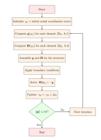
Physically, the Hessian matrix represents the tangent stiffness matrix in global coordinates. To solve Eq. (12), it is necessary to compute $g({\chi }_0)$ and $H\left({\chi }_0\right)$ as presented in Appendix A. Therefore, the Newton–Raphson iterative procedure can be summarized as follows:

1. Initialize ${\chi }_0$ as the initial nodal coordinates vector (undeformed configuration);

2. Compute $g({\chi }_0)$ for each element according to Eq. (A.1);

3. Compute $H\left({\chi }_0\right)$ for each element according to Eq. (A.2);

4. Assemble $g({\chi }_0)$ and $H\left({\chi }_0\right)$ for the structure by summing the contributions from each element;

5. Apply the boundary conditions;

6. Solve the resulting linear system according to Eq. (12) to find $�\chi$;

7. Update ${\chi }_0$ as ${\chi }_0={\chi }_0+\text{Δ}\chi$. Return to step 2 until $\left|\left|g\right|\right|\le tol$, where $tol$ is the specified tolerance.

Figure 2 illustrates this iterative procedure in flowchart form.

Figure 2
Flowchart of the Newton–Raphson iterative procedure within the positional formulation.

Mathematically, the previously presented procedure is non-incremental. However, decomposing the total load into successive steps (increments) facilitates the convergence of the solution, particularly in problems characterized by high nonlinearity. While this incremental procedure can be performed using the load control method, stability analyses requiring the tracing of the full equilibrium path necessitate alternative methods, such as displacement control or arc-length control.

In stability analyses using the present formulation, critical points, whether they are limit points or bifurcation points, are detected by the singularity of the Hessian matrix, characterized by the nullity of at least one eigenvalue. Thus, one has:

$$$$ $$\det \left[H({\chi }_0)\right]=0$$ (14)

However, when a critical condition is reached, a qualitative change in the equilibrium state occurs, which can be classified into three types:

(i) The total potential energy functional, $\text{Π}$, has a local minimum: $\det \left[H({\chi }_0)\right]>0$ (stable equilibrium state);

(ii) The total potential energy functional, $\text{Π}$, has a local maximum: $\det \left[H({\chi }_0)\right]<0$ (unstable equilibrium state);

(iii) The total potential energy functional, $\text{Π}$, is locally constant: $\det \left[H({\chi }_0)\right]=0$ (neutral equilibrium state).

3 NUMERICAL EXAMPLES

Three numerical examples are analyzed here. The first and second examples investigate the geometrically nonlinear behavior of a 2D two-bar truss and a 3D three-bar truss, respectively. The third example investigates the stability of a 24-bar star dome truss. In all examples, the stopping criterion for the iterative procedure was set to $tol=1.0\times {10}^{-8}$. For the numerical evaluation of the integral in Eq. (5) using the proposed element, 16 Gauss points were employed for members with variable axial rigidity and 1 Gauss point for members with constant rigidity.

3.1 2D Two-Bar Truss

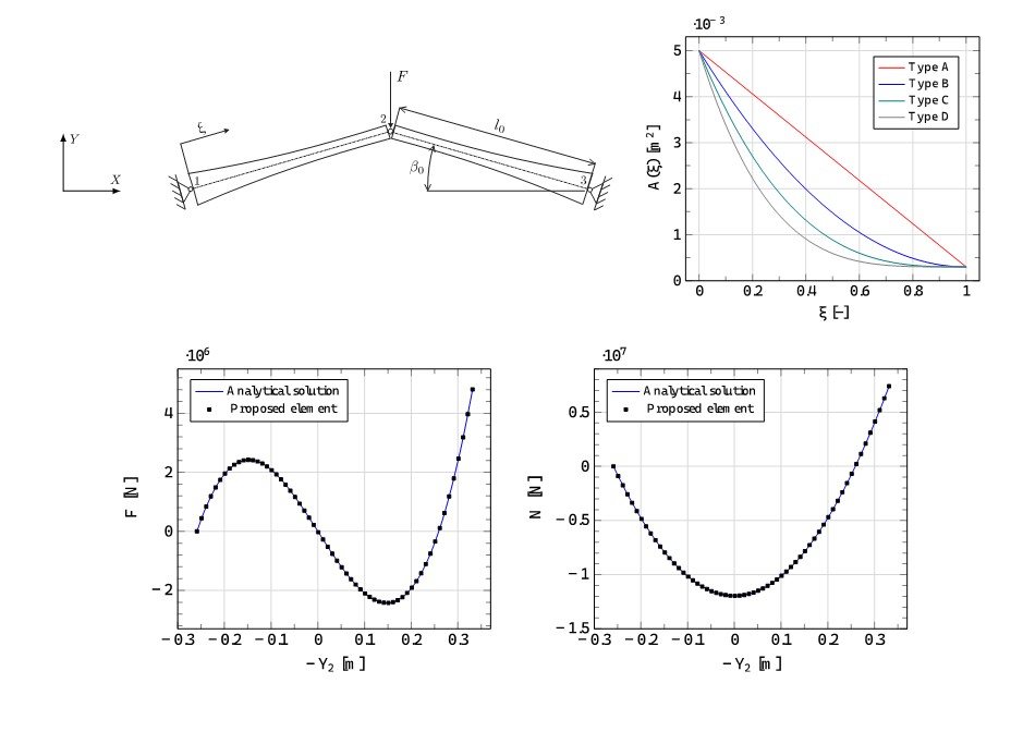
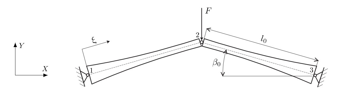
This example presents the geometrically nonlinear behavior of a 2D two-bar truss with polynomially variable axial rigidity (Figure 3), as presented in Kutis and Murín (2005). Each truss member is modeled using a single finite element. The member properties are defined by a Young's modulus of $E=2.1\times {10}^{11}$ Pa, and the geometric parameters $l_0=1$ m and ${\beta }_0=15°$.

Figure 3
Schematic of the 2D two-bar truss problem. Adapted from Kutis and Murín (2005).

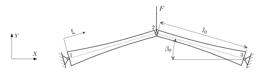
Four types of cross-sectional area variation are considered, with $A\left(\xi \right)$ given in m² by:

$$\begin{array}{l}\text{Type A:}A(\xi )=0.005-0.0047\xi \\ \\ \text{Type B:}A(\xi )=0.005-0.0094\xi +0.0047{\xi }^2\\ \\ \text{Type C:}A(\xi )=0.005-0.0141\xi +0.0141{\xi }^2-0.0047{\xi }^3\\ \\ \text{Type D:}A(\xi )=0.005-0.0188\xi +0.0282{\xi }^2-0.0188{\xi }^3+0.0047{\xi }^4\end{array}$$

Figure 4 illustrates the types of cross-sectional area variation along the dimensionless coordinate $\xi$.

Figure 4
Cross-sectional area as a function of the dimensionless coordinate $\xi$ for the various types.

The analytical solution for this problem is obtained by imposing equilibrium on the deformed configuration, assuming linear elastic material behavior. The same axial force $N$ acts along both bars and depends on the vertical position at the central node (node 2), denoted by $Y_2$, given by:

$$$$ $N=k_{11}{l}_0\left(\frac{\cos {\beta }_0}{\cos \beta }-1\right)$ (15)

where

$$\beta =\arctan \left(\frac{Y_2}{l_0\cos {\beta }_0}\right)$$

The axial stiffness coefficient $k_{11}$ in Eq. (15) is obtained analytically from Eq. (5). Therefore, the applied load $F$ is determined using Eq. (15) through the following expression:

$$$$ $F=-2N\sin \beta$ (16)

Table 1 shows the vertical displacement at node 2, denoted by $V_2$, for the four types of variation when applying a load of $F=6.0\times {10}^5$ N. The numerical results reported by Kutis and Murín (2005), using a single finite element per member, are also included in this table. Additionally, these authors analyzed this problem using 100 BEAM54 finite elements per member with the ANSYS® software. The load was applied in a single increment, where $N_{iter}$ is the number of iterations required.

Table 1
Comparison of vertical displacement at node 2 and number of iterations for the various types.

Type	Analytical solution		Proposed element		Kutis and Murín (2005)		Kutis and Murín (ANSYS®, 2005)
	$V_2$ [mm]	$N_{iter}$	$V_2$ [mm]	$N_{iter}$	$V_2$ [mm]	$N_{iter}$	$V_2$ [mm]	$N_{iter}$
A	13.780	-	13.780	5	13.927	9	13.777	10
B	27.860	-	27.860	6	28.490	12	27.854	13
C	40.818	-	40.818	6	42.165	15	40.811	17
D	52.300	-	52.300	6	54.635	19	52.290	21

The results in Table 1 highlight one of the key advantages of the proposed element: only one element per member is sufficient to reproduce the analytical solution, regardless of the axial rigidity variation. In contrast, the formulation by Kutis and Murín (2005), also using one element per member, exhibits significant errors, particularly for higher-order variations (types C and D). The mesh-refinement strategy in ANSYS® (100 BEAM54 elements per member) approaches the analytical solution, but at the cost of a substantial increase in the number of degrees of freedom and iterations. These findings demonstrate that, for trusses with variable axial rigidity, the proposed element eliminates the need for mesh refinement, providing a significant gain in computational efficiency without compromising accuracy.

Table 2 shows the vertical displacement at node 2 and residual norm, obtained using the proposed element, as functions of the iteration number when a load of $F=6.0\times {10}^5$ N is applied.

Table 2
Convergence of vertical displacement at node 2 and residual norm for the various types.

Type	Iteration	$V_2$ [mm]	$\left|\left|g\right|\right|$ [N]
A	1	12.766	6.00E+05
	2	13.774	4.10E+04
	3	13.780	2.49E+02
	4	13.780	9.46E-03
	5	13.780	8.27E-09
B	1	23.767	6.00E+05
	2	27.748	7.55E+04
	3	27.860	2.02E+03
	4	27.860	1.59E+00
	5	27.860	9.94E-07
	6	27.860	1.75E-09
C	1	32.140	6.00E+05
	2	40.268	1.01E+05
	3	40.816	6.02E+03
	4	40.818	2.69E+01
	5	40.818	5.43E-04
	6	40.818	8.27E-09
D	1	38.214	6.00E+05
	2	50.751	1.20E+05
	3	52.278	1.17E+04
	4	52.300	1.69E+02
	5	52.300	3.67E-02
	6	52.300	9.31E-10

According to Table 2, the proposed element converges before reaching the specified tolerance, requiring approximately 3–4 iterations for all types of variation.

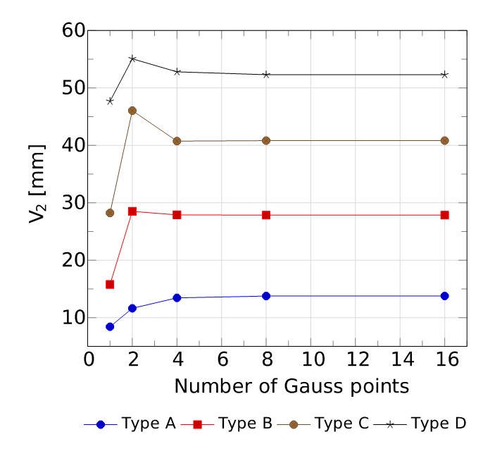
Figure 5 shows $V_2$, obtained using the proposed element, as a function of the number of Gauss points when a load of $F=6.0\times {10}^5$ N is applied.

Figure 5
Convergence of vertical displacement at node 2 with respect to the number of Gauss points for the various types.

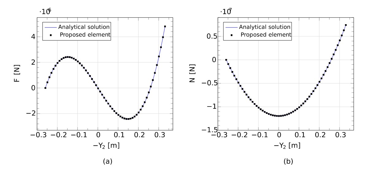
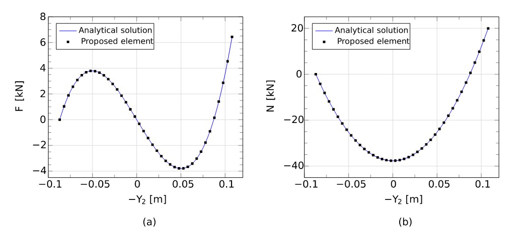
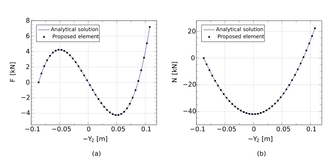
Figures 6through 9 show $F$ and $N$ as functions of $Y_2$. The solutions for the proposed element were obtained using the constant arc-length control method by applying arc length increments of $�S=1.0\times {10}^{-2}$ m.

Figure 6
Comparison of the equilibrium paths for type A: (a) Applied load vs. vertical position at node 2; (b) Axial force vs. vertical position at node 2.

Figure 9
Comparison of the equilibrium paths for type D: (a) Applied load vs. vertical position at node 2; (b) Axial force vs. vertical position at node 2.

Figure 7
Comparison of the equilibrium paths for type B: (a) Applied load vs. vertical position at node 2; (b) Axial force vs. vertical position at node 2.

Figure 8
Comparison of the equilibrium paths for type C: (a) Applied load vs. vertical position at node 2; (b) Axial force vs. vertical position at node 2.

Table 3 shows the limit load, $F_{LIM}$, obtained for the four types of variation.

Table 3
Comparison of limit load for the various types.

Type	Analytical solution	Proposed element
	$F_{LIM}$ [MN]	$F_{LIM}$ [MN]
A	2.42304	2.42304
B	1.30148	1.30148
C	0.96242	0.96242
D	0.80943	0.80943

3.2 3D Three-Bar Truss

This example presents the geometrically nonlinear behavior of a 3D three-bar truss with polynomially variable axial rigidity, as illustrated in Figure 10. Each truss member is modeled using a single finite element. The geometric parameters are as follows: $l_0=1$ m and ${\beta }_0=5°$.

Figure 10
Schematic of the 3D three-bar truss problem: (a) Top view; (b) Front view.

Five types of axial rigidity variation are considered, with $EA\left(\xi \right)$ given in kN by:

$$\begin{array}{l}\text{Type A:}EA(\xi )=1.0\times {10}^4(1-0.02\xi )\\ \\ \text{Type B:}EA(\xi )=1.1\times {10}^4(1-0.5\xi +0.66{\xi }^2)\\ \\ \text{Type C:}EA(\xi )=1.2\times {10}^4(1-0.98\xi +0.67{\xi }^2+0.89{\xi }^3)\\ \\ \text{Type D:}EA(\xi )=1.3\times {10}^4(1-2.03\xi +4{\xi }^2-2.67{\xi }^3+1.5{\xi }^4)\\ \\ \text{Type E:}EA(\xi )=1.4\times {10}^4(1-2.27\xi +6.72{\xi }^2-8.85{\xi }^3+3.91{\xi }^4+1.61{\xi }^5)\end{array}$$

Figure 11 illustrates the types of axial rigidity variation along the dimensionless coordinate $\xi$.

Figure 11
Axial rigidity as a function of the dimensionless coordinate $\xi$ for the various types.

The analytical solution for this problem is obtained by imposing equilibrium on the deformed configuration, assuming linear elastic material behavior. The axial force acting along the three bars is given by Eq. (15). Therefore, the applied load $F$ is determined using Eq. (15) through the following expression:

$$$$ $F=-3N\sin \beta$ (17)

Table 4 shows the vertical position at node 2 and residual norm, obtained using the proposed element, as functions of the iteration number for an applied load of $F=3.5$ kN. The load was applied in a single increment.

Table 4
Convergence of vertical position at node 2 and residual norm for the various types.

Type	Iteration	Analytical solution	Proposed element
		$Y_2$ [mm]	$Y_2$ [mm]	$\left|\left|g\right|\right|$ [kN]
A	1	-	71.6414	3.50E+00
	2	-	64.1271	8.74E-01
	3	-	61.6758	1.74E-01
	4	-	61.3788	1.70E-02
	5	-	61.3745	2.42E-04
	6	-	61.3745	5.22E-08
	7	61.3745	61.3745	2.26E-13
B	1	-	72.6964	3.50E+00
	2	-	66.5029	8.18E-01
	3	-	65.0801	1.29E-01
	4	-	65.0021	6.39E-03
	5	-	65.0018	1.89E-05
	6	65.0018	65.0018	1.67E-10
C	1	-	73.2481	3.50E+00
	2	-	67.6680	7.89E-01
	3	-	66.5896	1.10E-01
	4	-	66.5487	3.89E-03
	5	-	66.5487	5.54E-06
	6	66.5487	66.5487	1.13E-11
D	1	-	73.7664	3.50E+00
	2	-	68.7189	7.61E-01
	3	-	67.8861	9.46E-02
	4	-	67.8634	2.45E-03
	5	-	67.8634	1.81E-06
	6	67.8634	67.8634	5.60E-13
E	1	-	74.5595	3.50E+00
	2	-	70.2516	7.18E-01
	3	-	69.6907	7.43E-02
	4	-	69.6812	1.21E-03
	5	-	69.6812	3.39E-07
	6	69.6812	69.6812	1.55E-13

According to Table 4, the proposed element converges before reaching the specified tolerance, requiring approximately 4–5 iterations for all types of variation.

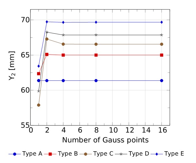
Figure 12 shows $Y_2$, obtained using the proposed element, as a function of the number of Gauss points for an applied load of $F=3.5$ kN.

Figure 12
Convergence of vertical position at node 2 with respect to the number of Gauss points for the various types.

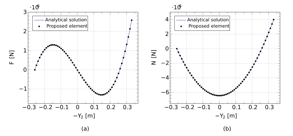
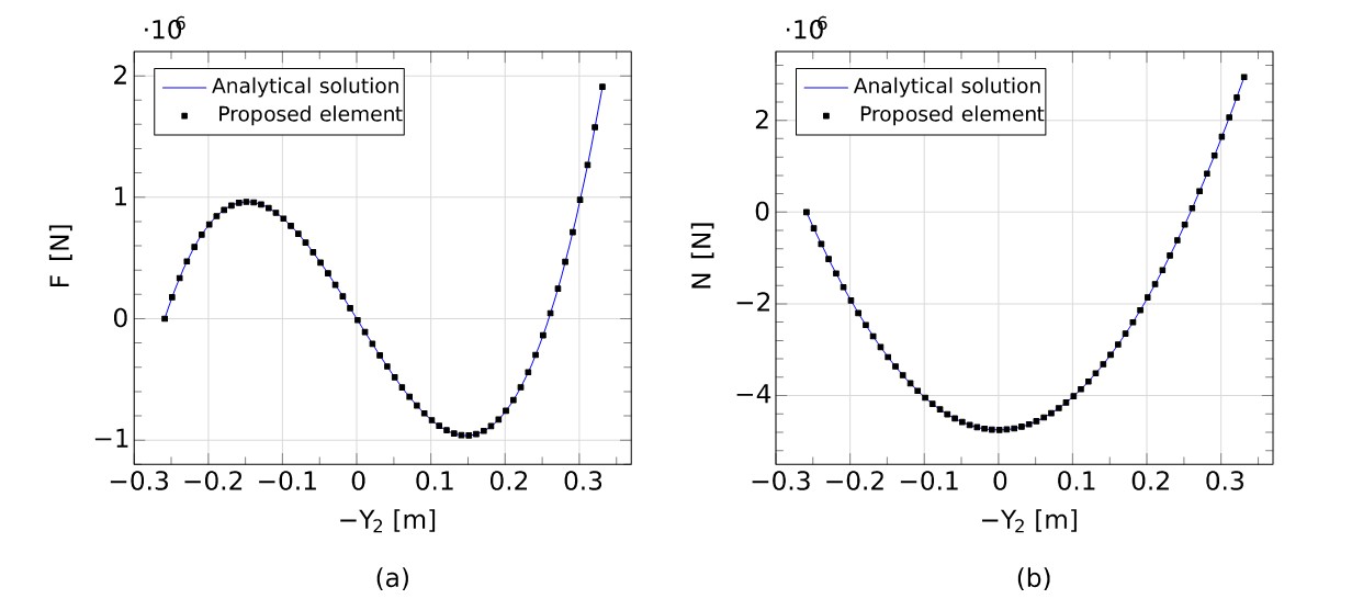
Figures 13through 17 show $F$ and $N$ as functions of $Y_2$. The solutions for the proposed element were obtained by applying arc length increments of $�S=5.0\times {10}^{-3}$ m.

Figure 13
Comparison of the equilibrium paths for type A: (a) Applied load vs. vertical position at node 2; (b) Axial force vs. vertical position at node 2.

Figure 17
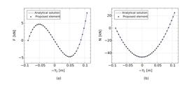
Comparison of the equilibrium paths for type E: (a) Applied load vs. vertical position at node 2; (b) Axial force vs. vertical position at node 2.

Figure 14
Comparison of the equilibrium paths for type B: (a) Applied load vs. vertical position at node 2; (b) Axial force vs. vertical position at node 2.

Figure 15
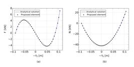
Comparison of the equilibrium paths for type C: (a) Applied load vs. vertical position at node 2; (b) Axial force vs. vertical position at node 2.

Figure 16
Comparison of the equilibrium paths for type D: (a) Applied load vs. vertical position at node 2; (b) Axial force vs. vertical position at node 2.

Table 5 shows the limit load, $F_{LIM}$, obtained for the five types of variation.

Table 5
Comparison of limit load for the various types.

Type	Analytical solution	Proposed element
	$F_{LIM}$ [kN]	$F_{LIM}$ [kN]
A	3.79841	3.79841
B	4.07558	4.07558
C	4.23724	4.23724
D	4.40126	4.40126
E	4.67838	4.67838

3.3 24-Bar Star Dome Truss

This example presents the stability analysis of a 24-bar star dome truss, as illustrated in Figure 18. Each truss member is modeled using a single finite element.

Figure 18
Schematic of the 24-bar star dome truss problem: (a) Top view; (b) Front view.

The bars connected to the supports (members a, with their nodes fixed at $\xi =0$) have an exponential axial rigidity variation, while the remaining bars (members b) have a constant rigidity, with $EA\left(\xi \right)$ expressed in kN as:

$$\begin{array}{l}\text{Members}a\text{:}EA(\xi )=1.5\times {10}^4{e}^{-\xi /4}\\ \\ \text{Members}b\text{:}EA=1.5\times {10}^4\end{array}$$

Figure 19 illustrates the axial rigidity variations along the dimensionless coordinate $\xi$ for members a and b.

Figure 19
Axial rigidity as a function of the dimensionless coordinate $\xi$ for members a and b.

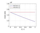
Figure 20 shows the axial flexibility $f_{11}$ of members a as a function of the number of Gauss points.

Figure 20
Convergence of axial flexibility for members a with respect to the number of Gauss points.

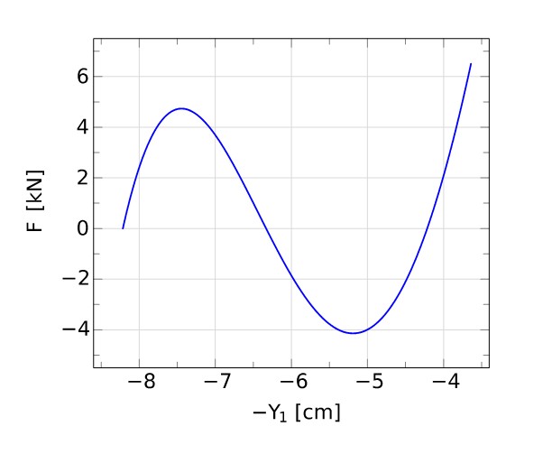
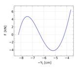
Figure 21 shows the equilibrium path obtained by applying arc length increments of $�S=5.0\times {10}^{-3}$ m using the proposed element. The obtained limit load was $F_{LIM}=4.73484$ kN, corresponding to a vertical position of $Y_1=7.44478$ cm.

Figure 21
Equilibrium path: Applied load vs. vertical position at node 1.

4 CONCLUSIONS

This paper presented the formulation and numerical validation of an exact geometrically nonlinear 3D truss finite element based on the positional formulation, capable of accounting for arbitrarily variable axial rigidity along the element's length.

The key advantage of the proposed formulation is its ability to accurately capture the geometrically nonlinear behavior of truss members using only a single finite element per member, regardless of the axial rigidity variation. This represents a significant computational efficiency gain compared to classical finite element software, which requires mesh refinement or multiple elements to approximate such variations.

A notable source of efficiency in the present formulation is its elimination of local-to-global coordinate transformations. By directly describing the equilibrium in the global coordinate system using nodal positions, the method avoids the computational overhead associated with the transformation of the Hessian matrix and internal force vector at each iteration, which is inherent in corotational or updated Lagrangian formulations. This simplifies the algorithm and reduces the computational cost per iteration.

The numerical examples demonstrated the exceptional accuracy and robustness of the proposed element. For both the 2D two-bar and 3D three-bar trusses with different types of polynomial axial rigidity variations, the results for displacements, positions, axial forces, and limit loads obtained with a single proposed element were in perfect agreement with the analytical solutions. Furthermore, the formulation exhibited faster convergence in the Newton–Raphson iterative procedure relative to existing methods from the literature.

The formulation's simplicity is also noteworthy, as it avoids deriving exact shape functions by directly utilizing the flexibility method and the PVF to compute the axial flexibility and employing numerical integration (Gauss quadrature) for general rigidity variations.

In summary, the proposed element proves to be a powerful, accurate, and efficient alternative for the geometrically nonlinear analysis of truss structures, combining the robustness of the positional formulation with the exact consideration of axial rigidity variation.

Appendix A  The residual force vector can be computed using the following expression:

$$$$ $$g({\chi }_0)=\left[\begin{array}{c}{f}_1\\ f_2\\ f_3\\ f_4\\ f_5\\ f_6\end{array}\right]-\left[\begin{array}{c}{F}_{X1}\\ F_{Y1}\\ F_{Z1}\\ F_{X2}\\ F_{Y2}\\ F_{Z2}\end{array}\right]$$ (A.1)

where

$$\begin{array}{l}{f}_1=k_{11}\left(1-\frac{l_0}{l}\right)(X_1-X_2)\\ \\ f_2=k_{11}\left(1-\frac{l_0}{l}\right)(Y_1-Y_2)\\ \\ f_3=k_{11}\left(1-\frac{l_0}{l}\right)(Z_1-Z_2)\\ \\ f_4=-f_1\\ \\ f_5=-f_2\\ \\ f_6=-f_3\end{array}$$

The Hessian matrix can be computed using the following expression:

$$$$ $$H({\chi }_0)=\left[\begin{array}{cccccc}{H}_{11}& H_{12}& H_{13}& H_{14}& H_{15}& H_{16}\\ & H_{22}& H_{23}& H_{24}& H_{25}& H_{26}\\ & & H_{33}& H_{34}& H_{35}& H_{36}\\ & & & H_{44}& H_{45}& H_{46}\\ & & & & H_{55}& H_{56}\\ \text{SYM}& & & & & H_{66}\end{array}\right]$$ (A.2)

where

$$\begin{array}{l}{H}_{11}=k_{11}\left\{1+\frac{l_0}{l}\left[{\left(\frac{X_2-X_1}{l}\right)}^2-1\right]\right\}\\ \\ H_{12}=k_{11}\frac{(X_2-X_1)(Y_2-Y_1)l_0}{l^3}\\ \\ H_{13}=k_{11}\frac{(X_2-X_1)(Z_2-Z_1)l_0}{l^3}\\ \\ H_{14}=-H_{11}\\ \\ H_{15}=-H_{12}\\ \\ H_{16}=-H_{13}\\ \\ H_{22}=k_{11}\left\{1+\frac{l_0}{l}\left[{\left(\frac{Y_2-Y_1}{l}\right)}^2-1\right]\right\}\\ \\ H_{23}=k_{11}\frac{(Y_2-Y_1)(Z_2-Z_1)l_0}{l^3}\\ \\ H_{24}=-H_{12}\\ \\ H_{25}=-H_{22}\\ \\ H_{26}=-H_{23}\\ \\ H_{33}=k_{11}\left\{1+\frac{l_0}{l}\left[{\left(\frac{Z_2-Z_1}{l}\right)}^2-1\right]\right\}\\ \\ H_{34}=-H_{13}\\ \\ H_{35}=-H_{23}\\ \\ H_{36}=-H_{33}\\ \\ H_{44}=H_{11}\\ \\ H_{45}=H_{12}\\ \\ H_{46}=H_{13}\\ \\ H_{55}=H_{22}\\ \\ H_{56}=H_{23}\\ \\ H_{66}=H_{33}\end{array}$$

Acknowledgments

This research was funded by CNPq (Conselho Nacional de Desenvolvimento Científico e Tecnológico) under grant number 302119/2022-1 and FAPEMIG (Fundação de Amparo à Pesquisa do Estado de Minas Gerais) under grant number 23072.229666/2022-13.

Data Availability statement:

No research data was used.

References

• Bathe, K.J., (2006). Finite Element Procedures. Klaus-Jurgen Bathe.
• Coda, H.B., Greco, M., (2004). A simple FEM formulation for large deflection 2D frame analysis based on position description. Computer Methods in Applied Mechanics and Engineering 193(33-35):3541-3557.
• Crisfield, M.A., (1991). Non-linear Finite Element Analysis of Solids and Structures. Volume 1: Essentials. John Wiley Sons, New York.
• Duris, R., Murín, J., (2007). A nonlinear truss finite element with varying stiffness. Applied and Computational Mechanics 1:417-426.
• Greco, M., Coda, H.B., (2006). Positional FEM formulation for flexible multi-body dynamic analysis. Journal of Sound and Vibration 290(3-5):1141-1174.
• Greco, M., Gesualdo, F.A.R., Venturini, W.S., Coda, H.B., (2006). Nonlinear positional formulation for space truss analysis. Finite elements in analysis and design 42(12):1079-1086.
• Greco, M., Menin, R.C.G., Ferreira, I.P., Barros, F.B., (2012). Comparison between two geometrical nonlinear methods for truss analyses. Structural Engineering and Mechanics 41(6):735-750.
• Greco, M., Ferreira, I.P., (2009). Logarithmic strain measure applied to the nonlinear positional formulation for space truss analysis. Finite elements in analysis and design 45(10):632-639.
• Greco, M., Peixoto, D.H.N., (2022). Comparative assessments of strain measures for nonlinear analysis of truss structures at large deformations. Engineering Computations 39(5):1621-1641.
• Greco, M., Venturini, W.S., (2006). Stability analysis of three-dimensional trusses. Latin American Journal of Solids and Structures 3(3):325-344.
• Khan, A.A., Alam, M.N., Rahman, N.U., Wajid, M., (2016). Finite element modelling for static and free vibration response of functionally graded beam. Latin American journal of solids and structures 13(4):690-714.
• Kutis, V., Murín, J., (2005). Bar element with variation of cross-section for geometric non-linear analysis. Journal of Computational and Applied Mechanics 6(1):83-94.
• Rabelo, J.M., Becho, J.S., Greco, M., Cimini Jr, C.A., (2018). Modeling the creep behavior of GRFP truss structures with Positional Finite Element Method. Latin American Journal of Solids and Structures 15(2):e17.
• Reddy, J.N., (2015). An Introduction to Nonlinear Finite Element Analysis: with applications to heat transfer, fluid mechanics, and solid mechanics. Oxford University Press.
• Saffari, H., Fadaee, M.J., Tabatabaei, R., (2008). Nonlinear analysis of space trusses using modified normal flow algorithm. Journal of structural engineering 134(6):998-1005.
• Shabana, A.A., (2020). Dynamics of Multibody Systems. 5th ed., Cambridge University Press.
• Silva, W.T., Ribeiro, K.B., Portela, A., (2024). Nonlinear analysis of spatial trusses with different strain measures and compressible solid. International Journal of Non-Linear Mechanics 167:104907.
• Souza, L.A.F., Santos, D.F., Kawamoto, R.Y.M., Vanalli, L., (2022). New fourth-order convergent algorithm for analysis of trusses with material and geometric nonlinearities. The Journal of Strain Analysis for Engineering Design 57(2):104-115.
• Thai, H.T., Kim, S.E., (2009). Large deflection inelastic analysis of space trusses using generalized displacement control method. Journal of Constructional Steel Research 65(10-11):1987-1994.

Edited by

• Editor:
  Marco L. Bittencourt

Publication Dates

• Publication in this collection
  27 Feb 2026
• Date of issue
  2026

History

• Received
  07 Nov 2025
• Reviewed
  02 Dec 2025
• Accepted
  08 Dec 2025
• Published
  10 Dec 2025