Bayesian-Optimized 5G Coverage Prediction using Geospatial ML with Feature Selection and K-Fold Evaluation

Abstract

The present research proposes a methodology to develop a model to predict Path Loss in a mixed environment comprising urban areas with tree-lined streets. Based on cross-validation and utilizing Artificial Intelligence (AI) and Machine Learning (ML) algorithms that employ various training functions, architectures, and numbers of neurons, the goal is to optimize the model’s performance in predicting Path Loss (PL) in mixed environments. The model is structured in layers, incorporating geolocation, non-line-of-sight loss, urban density, and vegetation coverage to predict PL. Within this model, Bayesian optimization is applied to select the best hyperparameters. Experimental results demonstrate its effectiveness, with a mean Root Mean Square Error (RMSE) per k-folds of 4.91 dB and Standard Deviation (STD) 4.76 dB for more forested areas.

Index Terms
5G; Amazon Region; Machine Learning; Path Loss Prediction

I. Introduction

The transition to the 5G (Fifth Generation) system provides a significant evolution in the Quality of Service (QoS) offered to users and the system’s overall architecture [¹]. With these changes, mobile network operators must meet the new demands of 5G users to ensure that the requirements of Long-Term Evolution (LTE) users are met, given the shared infrastructure characteristic of the transition [²]. For this purpose, researchers use several Path Loss (PL) models. However, these models cannot completely address the complexity of mixed environments, as evidenced by the results of the proposed model when compared to classical models [³].

This study used the drive test to collect real data. Drive test campaigns are widely used for data collection, as evidenced by several articles [⁴] [⁵] [⁶] [⁷]. These campaigns utilize G-NetTrack to analyze QoS and collect evaluation parameters, including Reference Signal Received Power (RSRP), Reference Signal Received Quality (RSRQ), and Signal-to-Interference-plus-Noise Ratio (SINR). We used the RSRP, in particular, to calculate the PL.

Recently, numerous studies have applied Machine Learning (ML) for prediction in mixed environments, employing multiple architectures and performance variables [⁸], geolocation as input [⁹], and line of sight as input for neural networks [¹⁰]. These studies use RSRP and different architectures to predict PL in Fourth Generation (4G) and 5G networks.

However, there is a lack of studies addressing the specific characteristics of the Amazonian environment. Furthermore, there is a scarcity of real field data compared to simulations, highlighting the need for greater methodological rigor, such as the use of k-folds based on Cell ID and explicit prevention of data leaks.

The current study investigates a mixed environment and applies PL models utilizing Artificial Intelligence (AI; Feedforward Network) and ML (Random Forest, Gradient Boosting (GBoost), and Support Vector Machine (SVM)). Additionally, multiple input features are also tested, including those already known in the literature, simplifications, and different forms of data acquisition for these input features. We collected, preprocessed, and analyzed the 5G signal levels obtained through measurement campaigns. RSRP, RSRQ, and SINR metrics were collected using two Next Generation NodeB (gN-odeBs) in Belém, Brazil. One gNodeB is in a region with extensive shadowing and a dense forested area, whereas the other is less diverse.

Finally, the AI and ML models were applied and optimized based on the scenario’s parameters and the proposed model’s cost function. This model enables the prediction of shadowed areas and the evaluation of signal adequacy in urban and vegetated environments.

Although PL models are currently employed in network planning, they frequently fail to capture the intricate propagation characteristics of mixed environments that include dense urban structures and tropical vegetation [¹¹]. Furthermore Ericsson, Alpha-Beta-Gamma (ABG), and Free Space are conventional empirical models that provide a valuable foundation, they are insufficiently sensitive to account for complex phenomena such as multipath fading and diverse shadowing in the current scenario. Additionally, many existing machine learning studies rely on simulated data or simplified scenarios that do not reflect real-world field complexities. This study addresses a gap in the literature, which is characterized by a significant lack of methodological rigor in the context of data leakage prevention, by implementing k-fold cross-validation partitioned by Cell ID. Our proposed method provides a more generalizable and robust solution by incorporating Bayesian-optimized algorithms with high-resolution geospatial layers, thereby addressing these deficiencies.

II. RELATED WORK

This model proposes a methodology to support network planning through a measurement campaign using a drive test, data pre-processing, analysis, geolocator software, and AI tools, such as neural networks, ML, such as Random Forest, and Bayesian methods. In this study, AI is applied to predict PL, and the models are trained by separating layers to reduce the complexity of the analysis.

A. Drive Test Campaigns

Widyasmoro [⁴] conducted a comparative study on the performance of 5G and 4G LTE networks in Jakarta, Indonesia, based on Signal Strength and QoS parameters. Similarly, [⁵] performed a driving test of mobile networks from existing operators in Ibra, Oman. Following these established methodologies, the present research adopts a similar data collection approach, utilizing the G-NetTrack software for data acquisition. Following these previous approaches, the present research a similar approach for data collection.

Studies such as those by Widyasmoro and Al’Jahami, demonstrate the importance of planning in the network evaluation. This study uses this information to fill in gaps, such as identifying shadowing areas and handover points. These works served as the basis for this initial analysis, which involved identifying and classifying the network’s Next Generation NodeB (gNodeB) and determining the node used.

In the context of PL acquisition data research, suburban modeling has been the subject of numerous articles and various data collection methods [¹²]. These methods include the use of uncrewed vehicles, such as drones, or, as previously mentioned, cars [¹³]. Both seek ways to better design, expand, and maintain networks in a given location, or create tools, such as models that predict the signal. This research, in contrast to its predecessors, employs G-NetTrack to conduct a drive test in an Amazonian environment.

B. AI, PL Prediction and Input Variables

Multiple studies analyze inputs, outputs, and hyperparameters to a neural network. These can be used as key performance parameters and show relevant results for each choice of input and output to the neural network.

• Use of multiple architectures: Paper [⁸] models PL using Multilayer Perceptron, applying different architectures and hyperparameters. From this, it is evident that the optimal number of hidden layers can be determined by adjusting the number of training samples, the number of hidden layers, and variables with environmental characteristics. Furthermore, the study considers the mean, mean square error, standard deviation, and correlation coefficient as performance measurement factors. This study differs from the work of Wu in that it relies on specific simplifications of urban areas in the Amazonian environment, rather than rasterization. Nevertheless, it integrates hyperparameter optimization by employing a custom cost function.

• Geolocation as input and multiple architectures: The work of Popoola [⁹] presents an extensive investigation using very high frequency, investigating various input variables, architectures, training functions, and algorithm types in PL prediction. Notably, geolocation is included among these inputs, emphasizing its relevance to the model.

• Line of sight as input to the neural network: the work of [¹⁰] uses a free line of sight propagation model in an urban environment. The probabilistic model employs a weighting function that determines the probability of line of sight for a specified separation distance between the transmitter and receiver. Similarly, the model adopted in this study simplifies the classification of whether an observer has a direct line of sight by utilizing the area generated by Google Earth, taking into account characteristics such as terrain and building heights.

• Singh [¹⁴] predicted the PL using Random Forest and achieved significant results compared to Artificial Neural Networks (ANN), with Mean Squared Errors (MSE) of 1.927 and 65.89, respectively. However, the study is applied in simpler scenarios and does not consider obstacles and complex environments, which this article addresses.

• Zhang’s approach [¹⁵] applies ML models (including Random Forest) for PL prediction in urban areas. Unlike this work, which used the grid search method, the present study applies Bayesian optimization. We also use the drive test for more complex, comprehensive routes and areas with diverse environments.

Therefore, this study considers a wide variety of factors within a novel environment, specifically the Amazon. Following the approach of AlHourani [¹²] focuses on modeling Cellular-to-UAV links in suburban settings through statistical excess PL based on the depression angle, our research introduces a layered geospatial framework specifically designed for terrestrial 5G propagation. We develop a unique PL model using Bayesian optimized AI and ML moving beyond traditional empirical approaches, the proposed model integrates high resolution inputs such as 3D building density, viewshed analysis. Inspired by previous works, we incorporate a diverse range of features, systematically select the most relevant ones, and subject the model to a rigorous cross-validation methodology.

III. Propagation Models

PL models are fundamental in wireless network planning, as they help determine the transmission power required to achieve the desired coverage and configure the network infrastructure [¹⁶]. With new technologies such as 5G and the upcoming 6G, currently in testing phases [¹⁷], network engineers can optimize network configurations by adjusting transmission power, antenna locations, and other parameters to maximize efficiency and coverage.

A. Free-space Model

The simplified form of the Free-space Model is expressed as Equation (1):

(1) $L\left(\text{dB}\right)=20{\log }_{10}\left(d\right)+20{\log }_{10}\left(f\right)+92.45,$

where L is PL in (dB), d is the distance in km, and f is the frequency in GHz. More advanced models may incorporate additional parameters for specific environmental characteristics, such as obstructions, reflections, and diffraction, among others [¹⁸].

B. ABG Model

The Alpha-Beta-Gamma (ABG) model describes PL for 5G mobile communication in urban scenarios, covering both micro and macro-cellular environments. Equation (2) defines the model:

(2) $P{L}^{ABG}\left(f,d\right)\left[\text{dB}\right]=10\alpha {\log }_{10}(\frac{d}{1\text{m}})+\beta +{10}_{\gamma }{\log }_{10}(\frac{f}{1\text{GHz}})+{\chi }_{\sigma }^{ABG},$

where ${\chi }_{\sigma }^{ABG}$ is the Standard Deviation describing large-scale signal fluctuations relative to the average PL over distance. The α, β, and γ are parameters obtained using closed-form solutions that minimize the standard deviation described by [¹⁹]. Where f is the frequency in GHz, and d is the distance in meters. This model provides the specific parameter values for each application scenario.

C. Ericsson Model

It is a modified version of the Okumura-Hata model, also known as Model 9999 [²⁰]. Its formula is given by the Equation (3):

(3) $P{L}_{9999}\left[\text{dB}\right]=a_0+a_1{\log }_{10}\left(d\right)+a_2{\log }_{10}\left(H_{AP}\right)+a_3{\log }_{10}\left(H_{AP}\right)x{\log }_{10}\left(d\right)-3.2{\left({\log }_{10}\left(11.75H_r\right)\right)}^2+g\left(f\right),$

where g(f) is the Equation (4):

(4) $g\left(f\right)=44.49{\log }_{10}\left(f\right)-4.78{\left({\log }_{10}\left(f\right)\right)}^2,$

and a₀, a₁, a₂, and a₃ are given by Table I. The model applies to 11 GHz, with the receiver’s height ranging from 2 to 10 meters and the transmitter’s height ranging from 10 to 80 meters, and a distance of 0.1 to 8 km between the two points. In the equation, H_r is the receiver’s height, H_AP is the transmitter’s height, and d is the distance between them.

Table I.
Parameter values of the Ericsson model [²⁰]

Area	a0	a1	a2	a3
Suburban	43.20	68.93	12	0.1
Urban	36.2	30.2	12	0.1
Rural	45.95	100.6	12	0.1

D. SS-RSRP

According to the technical standard [²¹] the SS-RSRP (Secondary Synchronization Signal Reference Signal Received Power) is the average of the power contributions (in Watts) of the resource elements that carry secondary synchronization signals (SS). In Frequency Range 1, the SS-RSRP is referenced to the antenna connector of the User Equipment (UE), whereas in Frequency Range 2, it is based on the combined signal from antenna elements that correspond to a specific receiver branch. In the current investigation, the SS-RSRP values collected via the G-NetTrack application are utilized directly as the RSRP variable in the link budget equation to estimate the PL.

E. SS-RSRQ

A 5G New Radio (NR) metric measures signal quality relative to total power. The 5G standard defines the SS-RSRQ (Secondary Synchronization Signal Reference Signal Received Quality) as the ratio of N × SS-RSRP to the NR carrier Received Signal Strength Indicator (RSSI), where N is the number of resource blocks in the measurement bandwidth [²¹]. The relationship is described in Equation (5). The present paper employs the generalized term RSRQ to denote the quality metric of both technologies, although the specific terminology for 5G is SS-RSRQ and for 4G is RSRQ.

(5) $\text{SS-RSRQ}=\frac{N\times \text{SS-RSRP}}{\text{NR}\text{carrier}\text{RSSI}}$

F. SS-SINR

The SS-SINR (Secondary Synchronization Signal Signal-to-Noise and Interference Ratio) is defined as the linear average of the power contribution (in Watts) of the resource elements carrying secondary synchronization signals divided by the linear average of the noise and interference power contribution over the same resource elements [²¹]. In order to ensure uniformity and simplification in the comparative tables of this work, the generic term SINR is employed to denote both metrics (4G SINR and SS-SINR 5G).

IV. Methodology

Fig. 1 illustrates the research process, which involves data filtering and the application of the proposed model. The data is collected by the G-netTrack application, filtered to remove reading errors, and preprocessed for use in the model. To prevent data leakage, the two gNodeBs are treated differently after being separated by Cell ID. The first gNodeB on Gentil Bitencourt Avenue (gNB-AG) is selected based on its best features using the feature importances attribute from Random Forest [²²], trained with k-folds per Cell ID using the cost function to choose the optimal hyperparameters, and then finalized with the best architecture. For the second dataset, gNodeB on Mundurucus Street (gNB-RM), we used the features and hyperparameters selected from the gNB-AG analysis to train the final network. Thus, although the search for the best features in gNB-AG may introduce some bias, when applied to gNB-RM, the results indicate the generalization of an unknown database.

Fig. 1.
Total flowchart of the experiment phases

The preprocessing is initially employed to eliminate samples that are identified as errors by the application (a PL reading of over 255 dB or Null). Following this, the 5G filter is implemented to separate samples from the N78 band. Cell ID is utilized to implement the IQR outlier removal method to address reading errors and signal fluctuations. Approximately 2.37% of the total samples in this study were impulsive noise and synchronization errors, which are eliminated by this statistical technique, which defines a normality interval.

To mitigate the effects of fast fading and reduce spatial autocorrelation, a Group 5 m strategy was implemented. This process entails the consolidation of regions with substantial overlap by spatially averaging samples within a 5 m radius. This step is crucial to prevent data leakage and ensure the model focuses on large-scale signal behavior (PL and shadowing).

This site-independent evaluation strategy, which has been implemented in this study, is designed to replicate a real-world network planning scenario. The model must be scalable to new regions without requiring a complete re-optimization process, as it has been developed for a single region. By performing feature selection and hyperparameter tuning exclusively on a single base station (gNB-AG), we ensure that the model identifies fundamental physical propagation patterns rather than site-specific geographical biases. This method offers a more rigorous proof of generalization than a combined dataset model, as the selection architecture can operate in a completely unseen environment via gNB-RM.

Although k-fold cross-validation within a single dataset is frequently adequate to prevent data leakage, geospatial propagation data frequently demonstrates high spatial autocorrelation [²³]. By employing gNB-AG as the primary environment for feature selection and gNB-RM as a completely unseen ‘blind test’ site, we assess the model’s capacity to generalize its learning to new geographical regions without the need for site-specific retraining. This approach emulates a realistic network planning scenario in which a pre-trained model is implemented in a new neighborhood.

A. Measurement campaign

The measurement campaign took place in the city of Belém do Pará, including five neighborhoods: Nazaré, Umarizal, São Brás, Guamá, and Cremação. We collected 4G and 5G signal data within a 1 km radius of the gNodeBs, which operated at 3.311 GHz with a 20 MHz bandwidth in the N78 band.

The drive test method was conducted at an average speed of 20 km/h with sunny weather, on a Sunday, and with low traffic between 1 PM and 7 PM. We utilized the G-NetTrack software [²⁴], two smartphones, and different 5G-compatible SIM cards. The routes traversed are marked in Fig. 2, as well as the gNodeBs given by name gNB-AG and gNB-RM. That methodology resulted in the collection of a total of 17,499 valid samples over 10 laps on the same route. This data was obtained through G-NetTrack, stored in the smartphones’ memory, and subsequently extracted for analysis.

Fig. 2.
Route traveled

Table II shows data collected from 4G and 5G in the area of interest on the ITU-R standards, including the overall RSRP, RSRQ, and SINR parameters. The columns include minimum, average, standard deviation, maximum values, and Confidence Interval (CI).

Table II.
Statistical comparison of RSRP, RSRQ, and SINR for 4G and 5G technologies with 95% confidence intervals

Parameter	Metric	4G	5G
RSRP (dBm)	Mean ± 95% CI Min/Max Std. Dev. CI Range	−86.688 ± 0.154 −113 / −60 8.747 [−86.842, −86.534]	−81.086 ± 0.276 −113 / 58 9.384 [−81.362, −80.811]
RSRQ (dB)	Mean ± 95% CI Min/Max Std. Dev. CI Range	−14.508 ± 0.055 −20 / −6 3.150 [−14.563, −14.452]	−11.923 ± 0.059 −26 / 11 2.022 [−11.982, −11.863]
SINR (dB)	Mean ± 95% CI Min/Max Std. Dev. Sample Count CI Range	−0.432 ± 0.067 −12 / 203.788 12385 [−0.499, −0.365]	18.005 ± 0.273 −7 / 30 9.027 4201 [17.732, 18.278]

Table II gives a preliminary statistical summary of the 4G and 5G signals throughout the entire measurement campaign in the Amazonian urban environment. Although these values aggregate heterogeneous conditions, they serve as a baseline for the technologies’ performance in the region. In subsequent modeling phases, the data is segmented by Cell ID and geospatial layers that isolate specific environmental factors to ensure a clear physical interpretation of the PL. These complexities, which include vegetation density, line of sight obstructions, and distance, are explicitly addressed and separated.

The dataset used for model training, validation, and testing was adopted from a previous study that also provides a comprehensive analysis of 4G and 5G signal coverage [⁶], [⁷]. It is important to clarify that although the signal level measurements (RSRP) utilized as the model’s target were adopted from a previous dataset, the earlier studies were strictly limited to descriptive statistical analyses of 5G and 4G coverage and QoS. Those preliminary works did not involve PL calculations, nor did they employ AI or ML techniques.

V. Planning Software

This work adapts the layer-based approach of Geographic Information Systems (GIS), separating the environment into multiple data layers for analysis [²⁵]. These layers represent various factors influencing the PL, including urban topography, line of sight from the reception point to the antenna, arborized and forested areas, geographical location, data collected from other sources, and specific antenna characteristics provided by the manufacturer. Fig. 3 illustrates the layer division based on the aforementioned factors in this research and will be used as input for the neural network.

Fig. 3.
Division into Layers. Source: Author

A. Geolocation Layer

This layer collects the geographic coordinates of the observation points and the radio base as input parameters for the neural network. Studies such as [⁹] and [²⁶] demonstrate the effectiveness of this methodology for predicting PL over distance. Subsequently, the distance was calculated from the radio base to the observer and between the observers’ points.

B. Urban Forested Zones Layer

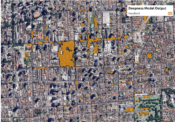
As another feature used as input for PL calculations, as in [²⁷], tree density is also considered complex in some propagation models. To extract data for the area of interest, we used the open-source software QGIS and the Deepness plugin [²⁸], which uses AI training and public data to separate data on various environmental factors, including trees.

By obtaining the location data of the trees and polygons, it was possible to process the tree density in a specific location. Fig. 4 shows the marking of the tree tops, which also contains geolocation information of the polygons.

Fig. 4.
Trees with geolocation extracted by Deepness Model

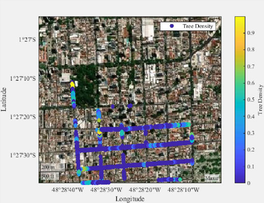
As a result, the density can be extracted as shown in Fig. 5 for gNB-AG and in Fig. 6 for gNB-RM.

Fig. 5.
Tree Density gNB-AG

Fig. 6.
Tree Density gNB-RM

C. Building Density Layer

The current layer calculates the number of buildings visible in the line of sight between the antenna and the receiver, as well as the area covered by buildings. In this context, PL results from several phenomena in signal propagation, including reflection, scattering attenuation, absorption, refraction, and diffraction, as the signal bypasses obstacles [²⁹]. These phenomena justify the use of these features.

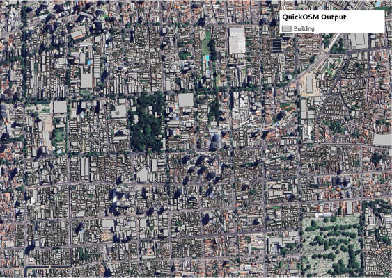
This layer calculates the density and number of buildings crossing a rectangle formed by the distance between the Transmitter (Tx) and Receiver (Rx), and with a width equal to the first Fresnel radius. This strategy is a simplification of the original Fresnel equation, which involves calculating only its first radius. This area counts both the number of buildings and the building density in the area. We extracted the data from QGIS’ QuickOSM, as shown in Fig. 7.

Fig. 7.
Buildings generated by Quickosm QGIS plugins

Using the same data, another feature is the number of buildings between Rx and Tx. Therefore, we obtain the distance to the first obstruction and its height. To achieve this, an initial height of 4 meters was applied to all houses, and corrections were made using Google Earth to form simplified building structures, as shown in Fig. 8.

Fig. 8.
3D polygons generated from heights and using Google Earth

Buildings were manually mapped using Google Earth, as shown in Fig. 8. Subsequently, the Keyhole Markup Language (KML) files were saved. This process enables the extraction of several key metrics: the distance to obstructions, the density of buildings over 9 meters in height (specifically within a 10-meter radius of the Rx, which significantly impacts shaded regions), the height of the first obstruction between the Tx and the Rx, the building density in the intervening area, and the total number of structures (e.g., houses or buildings) along the propagation path.

The feature building density, measured at a distance of 100m from Rx, serves as a critical environmental parameter for robust PL prediction models. Distances such as 10 or 50 meters might capture immediate, line of sight obstructions. However, they often fall short in adequately representing the complex multipath propagation phenomena prevalent in urban and suburban environments. A 100-meter radius offers a more comprehensive depiction of the local clutter, encompassing a broader range of structures responsible for significant reflections, diffractions, and scattering. This methodology enables the tested ML algorithms to more accurately correlate building density with the cumulative effects of physical interactions on radio wave attenuation, thereby leading to more accurate and generalizable PL estimations than those derived from more restrictive spatial considerations, as previous tests have shown using the dataset.

D. Viewshed Layer

Another important metric is whether or not there is a line of sight from the observation point to the transmitter. This metric is also used for the PL model in other works [³⁰].

This proposed model utilized Google Earth and its Visual Framing tool, which generates a viewshed from a specific point and height Fig. 9.

Fig. 9.
Viewshed using Google Earth gNB-AG. Source: Author

We performed the extraction using the image generated by Google Earth, as the application does not export this data directly. Therefore, image processing was done in Gimp to extract only the area of interest. To georeference the image (using QGIS), the Python code referenced the other points. The final work for gNB-AG can be seen in Fig. 10. Similarly, the same extraction methodology was performed in gNB-RM Fig. 11.

Fig. 10.
Viewshed extracted from gNB-AG

Fig. 11.
Viewshed extracted from gNB-RM

The original image has a resolution of 1024 by 768 pixels. This resolution is essential, as it allows for an efficient number of samples to be processed, clearly determining whether there is a direct line of sight. It is the minimum resolution permitted by Google Earth. With this resolution, we can confidently verify a direct line of sight with a precision of 2 meters between the test points.

However, the generated viewshed still lacks information, as it ignores, for example, newly constructed structures, such as a building with a significant obstruction less than 10 meters from the gNB-AG’s azimuth of 120°, which almost completely blocks the direct view of the site. To work around this, a Line of Sight Obstruction input was created, also based on the data in the Fig. 8.

Therefore, it was possible to have data more congruent with the reality of more recent obstructions. For gNB-AG, they can be seen in Fig. 12 with obstruction, 13 without obstructions, and for gNB-RM in Fig. 15 and 14 respectively with and without obstruction.

Fig. 12.
Obstruction line of sight gNB-AG

Fig. 13.
No Obstruction line of sight gNB-AG

Fig. 14.
Obstruction line of sight gNB-RM

Fig. 15.
No Obstruction gNB-RM

To calculate obstructions, the MATLAB function Inpolygon [³¹] checks if there is a polygon from the Rx to the Tx that represents the floor plan of the structures. If it is inside and it exceeds the line of sight, it is obstructed. Although limited, compared to software like Blender, it still presents good results consistent with the obstructions and tests carried out.

VI. COMPUTATIONAL INTELLIGENCE AND TECHNIQUES

Subsequent subsections will provide an overview of the data separation, processing, and optimization steps for AI and ML. Following the layered structure, this work implements AI and ML using Python and its various training functions.

A. Data processing by layer

Following the measurement campaign, we proceeded to the post-processing stage. The 5G data were separated into training, testing, and validation sets and subsequently normalized to facilitate neural network convergence. This overall workflow is illustrated in Fig. 1. For this phase, we utilized both Python and MATLAB: Python was employed to extract data from KML files and to handle model training and output generation, while MATLAB was used for the core data processing tasks.

Building upon the layer concept, specific calculations and functions were integrated into the data processing phase. Consequently, we extracted and processed the features required for model training, testing, and validation. Specifically, the Haversine formula [³²] was employed to independently calculate the distance between the gNodeB and each observation point. These spatial calculations constitute the first layer, which focuses on distance and location.

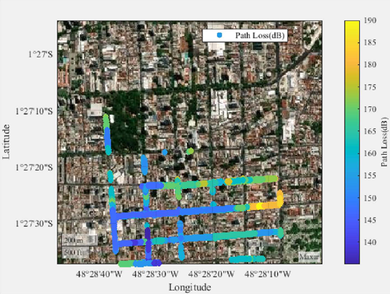
Filtering was necessary due to the large number of IDs of gNodeBs in the study area. Created in MATLAB to check which nodes are within the chosen perimeter and below a specific PL value, and close to the gNodeB (g-NetTrack has output showing where the gNB is possibly located). With this, possible candidate nodes are demarcated. As a result, the PL of the radio base of interest and its node were marked on the map with their respective data, as shown in Fig. 16 for gNB-AG and Fig. 17 for gNB-RM PL data.

Fig. 16.
Processed data used to output the PL network of the chosen gNB-AG and all Cell IDs. Source: Author

Fig. 17.
Path Loss all Cell IDs gNB-RM

The second layer, which represents vegetation, is based on numerous polygons. The vegetation density is calculated by determining the area of the treetops within a 10-meter radius of the Rx point and dividing it by the total area. As observed in the measurements, denser tree coverage correlates with higher PL. Furthermore, a building density layer was created to count the number of building intersections along an imaginary line toward the receiver, where n represents the number of buildings obstructing the path to the Rx. Additionally, a target layer for the base station was designed using the viewshed tool in Google Earth; any point within these generated polygons has a direct line of sight to the base station. Finally, to determine the output, the PL for each measurement point was calculated using the simplified Equation 6, following approaches in similar studies [²⁰], as expressed in:

(6) $RSR{P}_{\left(dBm\right)}=P_{RS}+G_{BS}-{\cancel{ATX}}^0+{\cancel{GUE}}^0-PL$

This simplification is necessary due to factors such as smartphone antenna gain, which varies from 0 to 5 dBi, depending on the country’s legislation and the manufacturer. We used a zero dBi omnidirectional antenna and a cable loss of 0 dB. In this way, the original equation is simplified to Equation (7), including the transformation of power in Watts to dBm, as shown in this equation:

(7) $P{L}_{\left(dB\right)}=10lo{g}_{10}\left(\frac{200W}{0.001}\right)+24-RSR{P}_{\left(dBm\right)},$

where RSRP - is the Reference Signal Received Power; P_RS - power reference signal in dBm; G_BS is transmitter antenna gain; ATX - Cable losses (0dB); GUE - is the receiver antenna gain (0 dBi) and PL- Path Loss.

Replacing the values with antenna data such as gain G_BS of (24dBi) and power (200W), we are left with the Equation (7).

Min-Max scaling was employed to normalize the target variable to improve the convergence of the training process. This technique maps the original values to the [0, 1] interval. This linear transformation was implemented using the Scikit-learn library in Python. Furthermore, the Path Loss data was filtered at the 1.5th percentile by Cell ID. Table III presents the number of removed samples, while the corresponding box plots for each Cell ID per respective gNB are shown in Fig. 18 and 19.

TABLE III.
Outliers removed per Cell ID after preprocessing

Cell ID	Outliers Removed	Total Samples
1	23	246
2	2	215
3	11	416
29	6	107
30	0	80
31	13	448
40	0	317
50	0	829
60	13	46
290	0	207
300	8	178
310	0	112
Total Outliers	76
Remaining Samples	–	3125 of 3201

Fig. 18.
Boxplot gNB-AG Cell IDs

Fig. 19.
Boxplot gNB-RM Cell IDs

The outlier detection rule follows the Interquartile Range (IQR) method. The IQR is a robust statistical technique used to define the normality interval within a dataset and identify anomalous samples [³⁴]. Applied per Cell ID, this threshold removes impulsive noise and synchronization errors, ensuring the quality of the training data for machine learning models. Although this method may eliminate extreme deep fade realizations, the subsequent spatial averaging guarantees that the model concentrates on large-scale signal behavior, including PL and shadowing.

The filtering has a negligible effect on shadowing statistics, as only 2.37% of the total samples were identified as outliers (as illustrated in Table III). Although deep fades are physically valid in multipath propagation, they denote small-scale fading phenomena that can serve as noise in large-scale PL models. The model successfully preserved the shadowing characteristics of a complex urban environment. As a consequence of eliminating these extreme values, the dataset’s physical integrity is preserved, which leads to a more consistent standard deviation and a higher correlation coefficient.

To prevent data leakage during model training and testing, samples belonging to the same Cell ID were grouped and spatially averaged. Even when samples from different Cell IDs (Cell Identifiers) were spatially close, the model did not group them. This preprocessing step alone increased the sample prediction correlation coefficient by filtering and consolidating regions with significant spatial overlap, thereby enhancing the prediction accuracy.

Although this approach smooths out fast-fading effects, it enhances the representation of large-scale signal behaviour (PL + shadowing), which is more relevant for the models trained. Spatial averaging is a common practice in propagation modelling and helps reduce short-term noise while preserving meaningful signal trends across space [³⁵] [³⁶].

For coverage modeling or calibrating PL models, the average is beneficial due to the results obtained. Using this strategy, the number of samples was reduced from 3,201 to 1,439, also reducing bias in some locations, as some sectors may have had more samples than others. Despite this, the network remained unbalanced in the number of samples per Cell ID, a common characteristic of real data.

B. AI and ML used

1) Random Forest: It is an ML model and an ensemble of bagged decision trees for regression and classification. By creating multiple decision trees during training, the output is the average of the predictions of the trees. Random forests reduce the effects of overfitting their training set [²²].

Random Forest is an ensemble-based model, widely recognised for its robustness and accuracy in regression and classification tasks. It uses multiple decision trees during training, which combine their predictions through voting (for classification) or averaging (for regression). It is well-regarded for its ability to resist overfitting and provide variable importance estimates, making it a practical choice for modelling complex and nonlinear phenomena [³⁷].

In this work, we use Random Forest as one of the comparative models, with its hyperparameters adjusted through Bayesian optimization to maximize predictive performance. Random Forest ML was the optimization result for the region near the forest with surplus areas, where the building almost completely blocked azimuth 120° on gNB-AG (one building was as close as 10m) or azimuth zero on gNB-RM, buildings were 100m away.

2) Gradient Boosting: Boosting-based ML sequentially combines weak models, which have shallow decision trees. At each iteration, the model corrects the errors made by previous iterations by minimizing a loss function through gradient descent. This approach enables the capture of complex, nonlinear patterns in the data. In this study, Gradient Boosting (GBoost) was used as one of the supervised learning models for PL prediction, with its hyperparameters optimized via Bayesian search to improve prediction accuracy and generalization [³⁸].

3) Feedforward Network: It is an artificial neural network architecture composed of sequentially arranged layers of neurons, through which information flows in a single direction. This structure is especially suitable for regression and classification tasks, and is used to model complex nonlinear relationships between input and output variables [³⁹]. In this work, the Feedforward Neural Network (FNN) is applied for PL estimation, trained with different subsets of input variables. Hyperparameters, such as the number of neurons and learning rate, were adjusted using Bayesian optimization.

4) Support Vector Machine: Support Vector Machine (SVM) is an ML method widely used in classification and regression tasks. Its core purpose is to find an optimal hyperplane that maximizes the margin between data from different classes (or minimizes the error in the case of regression). SVM is particularly robust in situations with limited data and exhibits good generalization capabilities, especially when combined with kernel functions [⁴⁰].

In this work, the SVM explores various kernel functions and optimizes their hyperparameters, including the regularization parameter C and the kernel coefficient, using Bayesian search techniques to maximize predictive performance.

C. Bayesian as an optimizer

The technique used for optimizing and training the neural network and Random Forest is Bayesian [⁴¹] [⁴²]. This research employed this technique, along with a cost function as presented in Equation (8), to analyze the various possibilities for both model structures:

(8) $\text{Cost}=\lambda \cdot {\text{MSE}}_{\text{Validation}}+\left(1+\lambda \right)\cdot {\text{STD}}_{\text{Validation}}$

Where our cost function combines both normalized MSE and Standard Deviation (STD). This normalization aims to prevent a single term from dominating due to its unit or scale, ensuring each contributes proportionally.

Subsequently, the coefficient Lambda (λ) is optimized using the same Bayesian optimization on the k-folds. This method allows for an efficient search for the optimal value of Lambda, adaptively weighting the relative importance of the normalized MSE and normalized standard deviation terms.

The model’s primary motivation is to develop a composite cost function that strictly penalizes variance and promotes better generalization by introducing an additional factor beyond the MSE. Although the Bayesian optimizer achieved λ=1 by effectively nullifying the STD term for the RF model, this result emphasizes the adaptive nature of the methodology. In addition, future research will explore the implementation of alternative cost functions to enhance the model across a diverse array of propagation scenarios.

D. About hyperparameters

The model applied the hyperparameters to tune the ML and AI models using Bayesian optimization. Additionally, all ML and AI models utilize a weighting parameter, denoted as Lambda (between 0 and 1), in the cost function.

In the Random Forest, the optimized hyperparameters included the number of estimators (50 and 500), maximum tree depth (5 and 30), minimum number of samples per split (2 and 10), minimum number of samples per leaf (1 and 30), and maximum number of variables considered per split (1 and 8).

Regarding the GBoost model, the optimized hyperparameters included the number of estimators, maximum depth, learning rate (0.0001 to 0.1), minimum number of samples per leaf, Lambda, and max features, with some ranges being similar to those used for Random Forest.

For FNN, the widths of up to six hidden layers (between 10 and 200 neurons or turned off if set to 0), as well as the learning rate, Lambda regularization parameter, and maximum number of iterations (10 to 1000). We also tested the Adaptive Moment Estimation (Adam), Limited-memory Broyden-Fletcher-Goldfarb-Shanno (L-BFGS), and Stochastic Gradient Descent (SGD) solvers using the same types of hyperparameters.

Finally, for the SVM model, the hyperparameters included the penalty cost C (between 0.1 and 1000), the epsilon parameter for the tolerance margin, gamma for the kernel (0.001 to 1), and kernel code that encodes the different kernels used (linear, poly, rbf, and sigmoid).

All models were tuned using Bayesian optimization, allowing for an efficient search of hyperparameter combinations that maximize predictive performance.

Common Settings for All Models:

• Validation strategy: Leave-one-Group-out, using Cell ID as the grouping variable and also separating gNB-AG and gNB-RM, and using only gNB-AG for optimization.

• Data normalization: Min-Max scaling applied only on the training subset in each fold.

• Random seed: random state equals 1 for reproducibility.

• Evaluation metrics: Pearson Correlation Coefficient (R), MSE, Mean Square Error (RMSE), STD, and Mean Absolute Error (MAE).

• Search Algorithm: Bayesian optimization

  • – Acquisition Function: Upper Confidence Bound (UCB)

  • – Exploration Parameter 0.01

  • – Iterations: 5 initial random points and 100 optimization iterations

  • – Stopping Criterion: Maximum number of iterations

E. Splitting raw data by gNodeBID

As already discussed in the section Data processing, the data obtained from the measurement campaign are from the PL of multiple base stations. The stations with the most significant amount of data are NodeIDs 913202 (433 samples), 9104030 (1,582 samples), and 910395 (1,779 samples). The investigation exclusively employed gNodeBs 9104030 (gNB-AG) and 910395 (gNB-RM).

The study will be based on massive Multiple Input, Multiple output (MIMo), and part of this prediction data will be analyzed with a single Cell ID to compare it with classic propagation loss models.

F. Search for better features

Inspired by related work, mainly due to the complexity of the urban landscape with extensive shaded areas, this model uses several inputs. Consequently, the use of Random Forest, which provides a function for input importance, facilitates the selection and reduces the number of combinations required to determine the optimal input parameter architecture. Fig. 20 shows all inputs and their importance levels using the gNB-AG dataset, divided into k-folds by Cell IDs.

Fig. 20.
Feature Importance Random Forest mean per k-folds(gNB-AG)

The gNB-AG was selected as the reference station for feature selection due to its increased environmental complexity. It is distinguished by dense forested regions and substantial urban shadowing. The justification is that if a subset of features can accurately capture PL in a worst-case propagation scenario, these variables are likely to remain robust when transferred to simpler or similar urban layouts. In contrast to a locally optimized but non-transferable model, this methodology places more emphasis on developing a feature set for the Amazonian urban environment.

To select the best features, highly correlated features with the absolute value of R greater than or equal to 0.6 are evaluated, as shown in Fig. 21. When two features are highly correlated, we remove the one with the lower importance score, as determined by the Random Forest model.

Fig. 21.
R between features in gNB-AG

Finally, the feature with the highest value in the importance graph generated by Random Forest is selected, as shown in Fig. 20. Those with equal importance will be separated based on their confidence level if necessary.

These steps to prevent multicollinearity and reduce model complexity result in improved performance, characterized by increased R-squared values and a decrease in error metrics.

Table IV shows features and how they are acquired. The geospatial and environmental parameters utilized as inputs are comprehensively described in this table, which also includes their physical significance and the methods of acquisition. The specific characteristics of the Amazonian environment are captured by these features, which are subsequently structured into input and output vectors for the learning models.

Table IV.
Description of input parameters used in the model

Column	Name	Description
Lat (col_0)	Latitude	Latitude of the receiver point
Lon (col_1)	Longitude	Longitude of the receiver point
Dist (col_6)	Distance	Haversine distance between the receiver and the specific gN-odeB
EA (col_15)	Elevation Angle	Calculated using the arctangent between the distance and the tower height
BDF (col_17)	Building Density (Fresnel)	Building area divided by the total area within a rectangle with length equal to Tx–Rx distance and width equal to the First Fresnel Zone radius
NBF (col_18)	Number of Buildings (Fresnel)	Number of buildings taller than 9 meters within the Fresnel zone defined by col_17
BD (col_16)	Building Density (Near Rx)	Number of buildings within a 100-meter radius around the receiver
FOH (col_5)	First Obstruction Height	Height of the first building that obstructs the direct path between Tx and Rx
HD (col_19)	Height Difference (Rx–Tx)	Height difference between receiver and transmitter, considering elevation data from [43]
RAz (col_9)	Relative Azimuth Position	Value of 1 if the point is aligned within the 120° sector of the Cell ID’s azimuth; 0 otherwise
DF (col_2)	Distance to First Obstruction	Distance to the first obstacle in the line of sight, extracted from 3D objects in Google Earth
TD (col_8)	Tree Density	Vegetation density within 10 meters of the receiver point, calculated using Deepness Model QGIS plugins
NB (col_3)	Number of Buildings in Line of Sight (LoS)	Number of buildings (not area) directly between Tx and Rx
LS_Obs (col_4)	Line of Sight Obstruction	Indicates whether there is any obstruction between Tx and Rx in a straight line
GEV (col_7)	Google Earth Viewshed	Viewshed analysis obtained through georeferenced image processing in Google Earth

In order to mathematically portray the relationship between signal attenuation and environmental variables, the input and output architectures are formally defined in Equations (9) and (10). The output vector, Y_out, denotes the predicted PL value, conversely, the input vector, X_in, aggregates the optimized subset of geospatial and environmental features, as detailed in Table IV.

(9) $X_{\text{in}}=\left[Lat,Lon,DF,Dist,TD,RAz,BD,BDF,HD\right]$

(10) $Y_{\text{out}}=\left[PathLoss\right],$

VII. Results and Discussion

The collected and filtered PL data from gNB-AG can be seen in Fig. 22, and for gNB-RM, it can be seen in Fig. 23 by Cell ID.

Fig. 22.
Path loss and distance gNB-AG

Fig. 23.
Path loss gNB-RM per distance

For instance, it is feasible to observe that Cell ID 2 experiences an increase in PL as distance increases; however, its PL begins to decline after 400 meters. The signal is enhanced by the significant reduction in tree density, which is a result of the change in environment.

It is also clear that Cell IDs with ample coverage (i.e., those reaching over 1,000 meters) exhibit a more pronounced pattern of PL increase with distance, similar to what is commonly observed in traditional PL models, as will be compared later. Cell IDs with less coverage have their PL altered by other physical factors, such as obstructions and other physical propagation phenomena.

This model removed two Cell IDs from gNB-AG because they significantly deviated from the other sets. This deviation resulted from signal obstruction by a building located less than 10 meters away at an azimuth of 120°. This building is taller than the radio base and has a large footprint. As a result, the physical phenomena affecting these signals are not representative, even with the extensive number of features analyzed in this study. Therefore, it is necessary to develop a separate model for situations where large obstructions are near the radio base.

A. Random Forest

The custom cost function was minimized through the application of Bayesian techniques during the optimization process for the RF model. Fig. 24 illustrates the convergence of this process over 100 iterations. Where the ‘Observation point’ represents the cost evaluated at each specific hyperparameter combination and the ‘Best Cost found’ indicates the progressive minimization of the error metric. The curve has stabilized, indicating that the optimizer has successfully identified an optimal region for the model’s hyperparameters.

Fig. 24.
Random Forest Optimization gNB-AG

The Bayesian optimization process on the gNB-AG dataset identified the optimal hyperparameters for the Random Forest regressor, which are summarized in Table V. The search algorithm converged after 100 iterations, stabilizing at a configuration that minimizes the custom cost function. The optimizer’s prioritization of the minimization of the Validation Mean Squared Error (MSE) is clear in the resulting Lambda (λ) of 1, which effectively adapts the model to the high complexity of the urban forested areas in the Amazonian region.

Table V.
Best hyperparameters found for the model (Random Forest)

Hyperparameter	Value
Lambda	1
max_depth	14
max_features	3
min_samples_leaf	1
min_samples_split	3
n_estimators	444

The average relative feature importance for the gNB-AG dataset is illustrated in Fig. 25. The primary predictors are spatial coordinates (col_0 and col_1, representing latitude and longitude, respectively) and distance (col_6). However, environmental factors such as building density within the Fresnel zone (col_17) also play a significant role.

Fig. 25.
Importance Random Forest gNB-AG per kfold with 95% confidence

This environmental influence is further corroborated by Fig. 26, which displays the feature importance for the gNB-RM dataset using a Random Forest model, although with a different distribution of significance. Together, these results demonstrate that the varying importance of specific features reflects the distinct physical characteristics of each site.

Fig. 26.
Importance Random Forest gNB-RM per kfold with 95% confidence

Using the hyperparameters found and the trained model, the results in Table VI for gNB-AG and Table VII for gNB-RM are obtained. These tables show the key metrics for each Cell ID, where N represents the number of samples. Table VII shows that even in cases where the number of samples per Cell ID was low, such as in Fold 6 with only 39 test samples, the model still achieves consistent predictive performance, maintaining a R of 0.773 and a relatively low RMSE of 4.15 dB. This finding highlights the Random Forest architecture’s resilience and the efficacy of the chosen geospatial features in capturing fundamental propagation patterns, even in the presence of restricted site-specific data.

Table VI.
Results per fold with performance metrics in training, validation, and test for gNB-AG

Fold (Cell ID)	Dataset	R	RMSE	MSE	N	STD	MAE
Fold 1 (2)	Training	0.975	1.82	3.30	360	1.82	1.36
	Validation	0.750	4.94	24.44	91	4.94	3.39
	Test	0.840	3.81	14.51	108	3.81	2.83
Fold 2 (30)	Training	0.977	1.65	2.73	402	1.65	1.20
	Validation	0.664	5.65	31.94	101	5.54	3.95
	Test	0.864	5.12	26.20	56	4.70	3.31
Fold 3 (31)	Training	0.983	1.49	2.21	289	1.49	1.01
	Validation	0.775	4.88	23.80	73	4.83	3.39
	Test	0.612	5.54	30.74	197	5.37	4.31
Fold 4 (3)	Training	0.979	1.75	3.06	288	1.75	1.19
	Validation	0.909	2.98	8.90	73	2.98	2.01
	Test	0.645	5.17	26.78	198	5.15	3.91

Table VII.
Results per fold with performance metrics in training, validation, and test for gNB-RM

Fold (Cell ID)	Dataset	R	RMSE	MSE	N	STD	MAE
Fold 1 (40)	Training	0.986	1.76	3.11	453	1.76	1.25
	Validation	0.898	4.65	21.61	114	4.63	3.13
	Test	0.671	7.50	56.24	134	7.00	5.73
Fold 2 (50)	Training	0.982	1.95	3.81	315	1.95	1.41
	Validation	0.895	4.21	17.69	79	4.20	3.09
	Test	0.854	5.54	30.69	307	5.50	4.39
Fold 3 (60)	Training	0.985	1.84	3.39	538	1.84	1.30
	Validation	0.923	3.99	15.93	135	3.99	2.92
	Test	0.525	5.02	25.19	28	4.83	3.73
Fold 4 (290)	Training	0.987	1.73	2.98	492	1.73	1.22
	Validation	0.890	4.52	20.41	123	4.52	3.29
	Test	0.586	7.17	51.43	86	7.17	6.13
Fold 5 (300)	Training	0.988	1.62	2.64	475	1.62	1.21
	Validation	0.911	4.20	17.63	119	4.19	3.07
	Test	0.770	7.39	54.61	107	7.12	4.81
Fold 6 (310)	Training	0.986	1.82	3.31	529	1.82	1.30
	Validation	0.891	4.59	21.11	133	4.50	3.38
	Test	0.773	4.15	17.18	39	4.08	3.29

The outlier Cell IDs are not discarded, despite the potential for ultimately leading to model improvements. Another example is Cell ID 290, which exhibits significant shadowing at a distance of 100 meters from azimuth 0.

The results of the other Cell IDs are also significantly influenced by the decision to maintain Cell IDs with obstructions that cause shadowing (e.g., large obstructions located near the base station but more than 10 m away). Excluding this data degrades model performance, but it also highlights its limitations.

The results show that the Random Forest model, although not specifically optimized for the gNB-RM scenario, demonstrates a remarkable learning capability. The high performance during the training phases (R > 0.98 in all folds), with consistently low RMSE, indicates that the model can adjust well to the training data. However, the discrepancy between the training, validation, and test results suggests a certain degree of overfitting, especially in cases where the test performance is significantly lower (for example, in Fold 1 and Fold 3).

Notably, the Bayesian optimization for the Random Forest model yielded a λ value of 1 (Table V), which mathematically concentrates the cost function entirely on the Validation MSE, effectively nullifying the contribution of the STD term. Although the composite cost function was intended to strictly penalize variance and enhance generalization, this outcome indicates that the optimizer prioritized error minimization for the RF architecture. This particular weighting implies that future models may benefit from a constrained λ range to guarantee the inclusion of the generalizationenhancing STD term.

Despite these results, hyperparameters and features selected from another model, such as the gNB-AG, through Bayesian optimization, are a strategic and efficient approach to avoid data leakage. This methodology allows for knowledge transfer and the exploration of features, providing a process that can accelerate the modeling and mitigate the need for exhaustive fine-tuning from scratch. Even with the variable performance across different Cell IDs during the testing phase, the model’s convergence and its ability to generalize in some folds (such as Fold 2 and Fold 6) demonstrate the promising potential of this transfer learning approach and the robustness of Random Forest, even under non-ideal fine-tuning conditions.

B. Gboost Optimization

The Bayesian optimization process for the GBoost model was executed. Fig. 27 illustrates the convergence of the cost function throughout the 100 iterations, where the algorithm identified the hyperparameter space that minimizes the weighted combination of validation error and variance.

Fig. 27.
Gboost optimization gNB-AG

The optimal configuration, which is detailed in Table VIII, is a compromise between the learning rate and the number of estimators that capture non-linear path loss patterns in Belém. These results, including a Lambda (λ) of 0.8736, confirm that the model effectively incorporated the standard deviation penalty to enhance its generalization capabilities across different neighborhoods.

Table VIII.
Best hyperparameters found for the model (Gboost)

Hyperparameter	Value
Lambda	0.8736
learning_rate	0.0621
max_depth	48
max_features	6
min_samples_leaf	7
n_estimators	263

C. Feedforward Network Bayesian Optimization

Table IX presents the results for each solver, using the same optimization method and the exact cost function. SGD was chosen as the solver because it demonstrates superior metrics.

Table IX.
Comparison of solvers’ performance on test set (95% confidence intervals)

Metric	Adam	L-BFGS	SGD
R	−0.0400 ± 0.12	0.5936 ± 0.21	0.4382 ± 0.18
RMSE (dB)	13.044 ± 1.85	8.594 ± 1.12	6.998 ± 0.95
MSE (dB)	204.9 ± 48.3	84.0 ± 18.9	50.4 ± 12.7
MAE (dB)	11.68 ± 2.15	6.047 ± 1.08	5.465 ± 0.92

The Feedforward was implemented using the ReLU activation function, with the SGD solver selected due to its superior performance metrics observed during preliminary tests. The Bayesian optimization process, illustrated in Fig. 28, was employed to determine the optimal configuration.

Fig. 28.
Feedforward Optimization gNB-AG using Solver SGD

The six hidden layers were selected by the Bayesian algorithm in this instance, suggesting a more complex network for the problem. The optimal hyperparameters, which encompass the specific neuron counts for each layer and the optimized learning rate necessary to simulate the non-linear path loss in the Amazonian urban environment, are delineated in Table X. The non-zero value for Lambda indicates that the weight parameter has once again influenced the hyperparameter selection, as demonstrated in the Gboost optimization.

Table X.
Best hyperparameters found for the deep neural network model (Feedforward)

Hyperparameter	Value
Lambda	0.9784
layer_1	115
layer_2	82
layer_3	68
layer_4	44
layer_5	59
layer_6	15
learning_rate	0.0517
max_iter	494

D. SVM Bayesian Optimization

The SVM model was optimized using an SVR architecture to handle the non-linearities of the propagation environment. The Bayesian optimization focused on tuning the penalty cost C, the epsilon tolerance margin, and the kernel coefficient gamma to find the best hyperplane for path loss prediction. As shown in Fig. 29, the cost function reached stability by identifying a configuration that minimizes the weighted combination of error and variance.

Fig. 29.
SVM optimization gNB-AG

Table XI provides a comprehensive breakdown of the final hyperparameters, which encompass a linear kernel and a Lambda (λ) of 0.9071. This ensures that the model retains its generalization capability, even in the presence of the restricted data that is typical of real-world drive tests.

Table XI.
Best hyperparameters found for the SVR model

Hyperparameter	Value
Lambda	0.9071
C	92
epsilon	0.218
gamma	0.2795
kernel	linear

E. Comparison between mean values of ML and AI

To ensure a focused analysis of the most effective solution, detailed per-fold results will be presented specifically for the RF model, which demonstrated the highest predictive accuracy and stability across both gNBs datasets. In the comparative section, the models’ performance is mainly presented using mean metrics and confidence intervals. The models (GBoost, FNN, and SVM) also underwent the same exacting k-fold cross-validation procedure to stop data leakage and use the same features chosen for the RF model. The objective of this reporting strategy was to emphasize the superior Random Forest architecture’s robust behavior and reliability in managing the intricate Amazonian geospatial features, and simultaneously preserve compactness by employing the other models as comparative benchmarks.

The methodology was developed to assess the model’s ability to generalize across different sites. Fig. 30 illustrates the outcomes for gNB-AG, which was the primary optimization dataset for feature selection and Bayesian hyperparameter tuning.

Fig. 30.
Average performance per k-fold with 95% confidence interval across train, validation, and Test sets (gNB-AG)

In contrast, Fig. 31 presents the performance on gNB-RM, which acted as a ‘blind test’ site.

Fig. 31.
Average performance per k-fold with 95% confidence interval across TRAIN, VAL, and TEST sets (gNB-RM)

For this second dataset, the model utilized the exact hyperparameters and features previously optimized on gNB-AG without further site-specific optimization of the hyperparameters. This approach ensures that the model identifies fundamental physical propagation patterns rather than site-specific biases, thereby replicating a realistic network planning scenario where a pre-trained model is deployed in a new geographical region.

The superiority of the RF model is quantitatively validated by the results in Tables VI and VII, which present consistent performance across all k-folds for both gNB-AG and gNB-RM. Random Forest performed best in both scenarios, exhibiting the highest average correlation coefficients on the test dataset (R = 0.740 on gNB-AG and R = 0.696 on gNB-RM) and the lowest average errors on the test set (RMSE = 4.91 and 6.13, respectively). Furthermore, the comparative analysis illustrated in Fig. 30 and 31 confirms that RF maintains higher stability and accuracy compared to GBoost, SVM, and FNN, demonstrating its robust generalization capability even in the presence of complex Amazonian geospatial features.

These results demonstrate strong generalization ability. Gradient Boosting performed similarly, but with a slight increase in squared and absolute errors. On the gNB-AG dataset, it obtained R = 0.711 and RMSE = 5.13 in the test. For gNB-RM, the results were R = 0.697 and RMSE = 6.05 dB. The SVM performed intermediately, outperforming the FNN in all test scenarios, particularly in gNB-RM (R = 0.499, RMSE = 10.63). In gNB-AG, the SVM obtained R = 0.252 and RMSE = 7.61.

On the other hand, the Feedforward performed worse overall, especially in gNB-AG (R = 0.438 and RMSE = 7.00), indicating limitations in capturing the complex spatial patterns of these urban environments. In gNB-RM, it obtained R = 0.583 and RMSE = 7.70. The comparison graphs visually reinforce the consistency of Random Forest as the most robust model among those tested.

The gNB-AG approach brings lower confidence intervals, indicating greater stability, especially for Random Forest and Gradient Boosting. In contrast, the wider intervals in gNB-RM using Feedforward or SVM suggest reduced consistency. Notably, Random Forest remained stable in both cases. Additionally, the gNB-RM scenario features fewer trees and lower building density, which helps mitigate environmental variability and model complexity. However, despite this simpler propagation environment, the lack of dynamic adjustment in gNB-RM resulted in lower average performance and less reliable predictions for most models, without the risk of data leaks.

F. Applying the network for prediction in the area of interest

The Out of Fold (OOF) predictions were employed to generate the results depicted in Fig. 32, 33, and 34, which were then compared to traditional PL models. In this procedure, the dataset was partitioned into k folds based on Cell ID. A model instance was trained on k-1 folds for each iteration and subsequently employed to forecast the path loss for the remaining held-out fold. By aggregating these independent test predictions, we obtained a complete set of predicted values for the study area where no sample was ever used in its training phase. This methodology aims to eliminate data leakage and ensures that the comparative analysis against empirical benchmarks reflects the true generalization capability of the Random Forest model in the Amazonian urban environment.

Fig. 32.
Comparison of prediction with classical and original PL models gNB-AG

Fig. 33.
Comparison of prediction with classical and original PL models using gNB-RM

Fig. 34.
PL Random Forest Prediction and Original Data

3D Plot: Latitude x Longitude x PL

The empirical models, Free Space, Ericsson, and ABG, provide a valuable baseline. Their behavior is distance-dependent and smooth, but it is unable to capture the sharp signal fluctuations that are observed in the field. By comparison, the predictions of the machine learning model exhibit superior sensitivity to local environmental changes, closely matching the measured signal levels across a variety of Cell IDs. A clear example is seen in Cell ID 2, where the model accurately predicts a decrease in path loss after 400 meters, corresponding to a localized reduction in tree density that improved signal propagation.This emphasizes the efficacy of the layered geospatial approach in simulating intricate urban environments in the Amazon, where distance alone is insufficient as a predictor.

The 3D plot in Fig. 34 offers a comprehensive representation of the predicted versus original PL data throughout the entire area of interest. The results suggest a high degree of fidelity, as the predicted values consistently remain near the collected field samples. It’s noteworthy that even between geographically close points, the visualization shows notable signal variations. Complex physical phenomena, including multipath fading, reflection, and shadowing, which are caused by dense vegetation and irregular urban topography, are the primary causes of these fluctuations. The RF model was able to efficiently learn the underlying propagation patterns, thereby ensuring that the predictions were robust across the study region, despite the heterogeneous conditions.

VIII. Conclusion

With the advancement of 5G networks and their new possibilities in various applications across multiple areas, including health, Industry 4.0, and IoT, studies analyzing urban network coverage in areas with dense vegetation, such as the Amazon region, are essential.

Field research is essential for gaining a better understanding of the performance of both technologies, which are in a transition phase, and for contributing to the improvement of planning and implementation of next-generation networks, particularly in regions with unique characteristics, such as the Amazon region.

The research presented here proposes a methodology for developing a model to predict PL in 5G urban environments with mixed settings, utilizing real-world data collected through drive test in the Amazon region. The model uses a layered input structure to incorporate relevant geospatial and environmental features, including building and vegetation density, distance to the transmitter, and viewshed analysis. All these features were processed to prevent data leakage and normalized to support robust model training.

Among the evaluated models—Feedforward Neural Network, Support Vector Machine, Gradient Boosting, and Random Forest—Gradient Boosting and Random Forest are the two tree-based ensemble models. Based on the results and comparisons, Random Forest demonstrated superior performance in terms of generalization and accuracy.

Using Bayesian optimization for hyperparameter tuning, Random Forest achieved the highest average correlation coefficient and the lowest RMSE across multiple k-folds and gNodeBs. Despite the lower R in some Cell IDs, the models still delivered solid performance according to other statistical metrics, such as RMSE, MAE, and STD. These results indicate that the models are capable of capturing complex propagation behaviors and producing reliable predictions, even in heterogeneous and challenging environments.

This proposed methodology can be applied to other locations, allowing for scalability in the cellular network’s demand and expanding studies to more complex and robust scenarios. However, a new analysis is necessary. When training the AI or ML model with a new radio base station, it is crucial to create a new viewshed and retrain the network.

In future work, we plan to evaluate additional parameters such as throughput, downlink, and uplink in 5G networks. Another necessary improvement involves developing detailed terrain and building models using Blender and ray tracing. This approach aims to minimize the oversimplification of 3D structures and better represent real-world features.

ACKNOWLEDGMENTS

This work was supported in part by the Coordination for the Improvement of Higher Education Personnel - Brazil (CAPES), under Financing Code 001, and by the Federal University through the Graduate Program in Electrical Engineering (PPGEE). The authors also thank the students, faculty, and collaborators of LCT for their valuable support.

Data Availability

The raw signal metrics (RSRP, RSRQ, and SINR) that support the findings of this work were adopted from previous measurement campaigns conducted by the Laboratory of Computing and Telecommunications (LCT) at UFPA, as described in [6] and [7]. These datasets were strictly limited to descriptive statistical analyses and did not include the PL calculations or the IA and ML models developed in the present work. The data are available from the corresponding author upon reasonable request.

REFERENCES

• ¹ M. Attaran, “The impact of 5G on the evolution of intelligent automation and industry digitization,” Journal of Ambient Intelligence and Humanized Computing, vol. 14, no. 5, pp. 5977–5993, 2023. [Online]. Available: https://doi.org/10.1007/s12652-020-02521-x
  » https://doi.org/10.1007/s12652-020-02521-x
• ² C. Henrique, A. Jr., and L. Pereira, “Coexistência entre 5G NR e LTE-A em sistemas Fiber/Wireless,” XXXVIII Simpósio Brasileiro de Telecomunicações e Processamento de Sinais, pp. 1 570649771:1–1 570649771:4, 2020. [Online]. Available: https://www.sbrt.org.br/sbrt2020/papers/1570649771.pdf
  » https://www.sbrt.org.br/sbrt2020/papers/1570649771.pdf
• ³ Y. Ma, W. Li, D. Han, Y. He, Q. Li, X. Bai, and D. Xu, “Wireless wave attenuation in forests: An overview of models,” Forests, vol. 15, no. 9, pp. 1587:1–1587:24, 2024. [Online]. Available: https://www.mdpi.com/1999-4907/15/9/1587
  » https://www.mdpi.com/1999-4907/15/9/1587
• ⁴ Widyasmoro, I. Surahmat, T. K. Hariadi, and F. Dwi Putra, “Comparative performance analysis of 4G and 5G cellular network technology in indonesia: Case study in the city of Jakarta,” 2nd International Conference on Electronic and Electrical Engineering and Intelligent System, pp. 158–163, 2022.
• ⁵ M. A. A. Jahdhami and et al., “Performance analysis of mobile broadband networks in Ibra city, Oman,” International Conference on Artificial Intelligence and Big Data Analytics, pp. 1–6, 2021.
• ⁶ V. Filho, Y. Sousa, and et al., “Análise comparativa de cobertura e qualidade entre as redes celulares 4G e 5G em Belém-PA,” XIII Conferência Nacional em Comunicações, Redes e Segurança da Informação, pp. 17–18, 2023.
• ⁷ V. Filho and et al., “Análise de cobertura e qualidade de rede celular 5G: Estudo de caso de Belém-PA,” XIV Conferência Nacional em Comunicações, Redes e Segurança da Informação, pp. 21–22, 2023.
• ⁸ L. Wu, D. He, B. Ai, J. Wang, H. Qi, K. Guan, and Z. Zhong, “Artificial neural network based path loss prediction for wireless communication network,” Institute of Electrical and Electronics Engineers Access, vol. 8, pp. 199 523–199 538, 2020.
• ⁹ S. I. Popoola, A. Jefia, A. A. Atayero, O. Kingsley, N. Faruk, O. F. Oseni, and R. O. Abolade, “Determination of neural network parameters for path loss prediction in very high frequency wireless channel,” Institute ofElectrical and Electronics Engineers Access, vol. 7, pp. 150 462–150 483, 2019.
• ¹⁰ H. Cheng, S. Ma, H. Lee, and M. Cho, “Millimeter wave path loss modeling for 5G communications using deep learning with dilated convolution and attention,” Institute of Electrical and Electronics Engineers Access, vol. 9, pp. 62 867–62879, 2021.
• ¹¹ C. M. M. Cardoso, B. S. d. S. Barbosa, A. S. Macedo, H. A. O. da Cruz, F. C. Fernandes, F. J. B. Barros, and J. P. L. e Araujo, “Estimating attenuation coefficients in wooded environments with ann predictions,” Institute of Electrical and Electronics Engineers Access, vol. 13, pp. 144 941–144 953, 2025.
• ¹² A. Al-Hourani and K. Gomez, “Modeling cellular-to-uav path-loss for suburban environments,” Institute of Electrical and Electronics Engineers Wireless Communications Letters, vol. 7, no. 1, pp. 82–85, 2018.
• ¹³ H. Zheng, W. Li, L. Tian, C. Xu, F. Huang, and J. Zhang, “Path loss models for urban macro cell scenario at 3.35, 4.9 and 5.4 GHz,” Institute of Electrical and Electronics Engineers 26th Annual International Symposium on Personal, Indoor, and Mobile Radio Communications, pp. 2229–2233, 2015.
• ¹⁴ H. Singh, S. Gupta, C. Dhawan, and A. Mishra, “Path loss prediction in smart campus environment: Machine learning-based approaches,” Institute of Electrical and Electronics Engineers 91st Vehicular Technology Conference, pp. 1–5, 2020.
• ¹⁵ Y. Zhang, J. Wen, G. Yang, Z. He, and J. Wang, “Path loss prediction based on machine learning: Principle, method, and data expansion,” Applied Sciences, vol. 9, no. 9, pp. 1908–1908, 2019. [Online]. Available: https://www.mdpi.com/2076-3417/9/9/1908
  » https://www.mdpi.com/2076-3417/9/9/1908
• ¹⁶ A. Ikpehai, B. Adebisi, K. M. Rabie, K. Anoh, R. E. Ande, M. Hammoudeh, H. Gacanin, and U. M. Mbanaso, “Low-power wide area network technologies for internet-of-things: A comparative review,” Internet of Things Journal, vol. 6, no. 2, pp. 2225–2240, 2019.
• ¹⁷ P. Tang, J. Zhang, H. Tian, Z. Chang, J. Men, Y. Zhang, L. Tian, L. Xia, Q. Wang, and J. He, “Channel measurement and path loss modeling from 220 GHz to 330 GHz for 6G wireless communications,” China Communications, vol. 18, no. 5, pp. 19–32, 2021.
• ¹⁸ M. Veletic and M. Sunjevaric, “On the cramer-rao lower bound for rss-based positioning in wireless cellular networks,” International Journal of Electronics and Communications, vol. 68, no. 8, pp. 730–736, 2014.
• ¹⁹ S. Sun, T. S. Rappaport, S. Rangan, T. A. Thomas, A. Ghosh, I. Z. Kovacs, I. Rodriguez, O. Koymen, A. Partyka, and J. Jarvelainen, “Propagation path loss models for 5G urban micro- and macro-cellular scenarios,” Institute of Electrical and Electronics Engineers 83rd Vehicular Technology Conference, pp. 7 504435:1–7 504435:6, 2016.
• ²⁰ Z. E. Khaled, W. Ajib, and H. Mcheick, “An accurate empirical path loss model for heterogeneous fixed wireless networks below 5.8 GHz frequencies,” Institute of Electrical and Electronics Engineers Access, vol. 8, pp. 182755–182775, 2020.
• ²¹ ETSI, “5G; NR; Physical layer measurements (3GPP TS 38.215 version 15.2.0 Release 15),” European Telecommunications Standards Institute, Technical Specification ETSI TS 138 215 V15.2.0, 2018. [Online]. Available: https://www.etsi.org/deliver/etsi_ts/138200_138299/138215/15.02.00_60/ts_138215v150200p.pdf
  » https://www.etsi.org/deliver/etsi_ts/138200_138299/138215/15.02.00_60/ts_138215v150200p.pdf
• ²² The scikit-learn developers, “Scikit-learn documentation: Random forest regressor,” 2025. [Online]. Available: https://scikit-learn.org/stable/modules/generated/sklearn.ensemble.RandomForestRegressor.html
  » https://scikit-learn.org/stable/modules/generated/sklearn.ensemble.RandomForestRegressor.html
• ²³ S. M. Alhammad, M. M. Eid, E. A. Mattar, and E.-S. M. El-Kenawy, “Optimization-driven learning for leakage-controlled geospatial modeling of antenna structure registration data,” Institute ofElectrical and Electronics Engineers Access, vol. 14, pp. 15 273–15310, 2026.
• ²⁴ G. Solutions. (2023) G-NetTrack Pro. [Online]. Available: https://gyokovsolutions.com/
  » https://gyokovsolutions.com/
• ²⁵ Pathloss. (2023) Pathloss 6. [Online]. Available: https://www.pathloss.com/pathloss6.html
  » https://www.pathloss.com/pathloss6.html
• ²⁶ I. Yazici and E. Gures, “A robust machine learning approach for path loss prediction in 5G networks with nested cross validation,” 10th International Conference on Wireless Networks and Mobile Communications, pp. 1–6, 2023.
• ²⁷ J. C. Silva, G. L. Siqueira, and P. V. G. Castellanos, “Propagation model for path loss through vegetated environments at 700 – 800 MHz band,” Journal of Microwaves, Optoelectronics and Electromagnetic Applications, vol. 17, no. 1, pp. 179–187, 2018.
• ²⁸ P. Aszkowski, B. Ptak, M. Kraft, D. Pieczyński, and P. Drapikowski, “Deepness: Deep neural remote sensing plugin for QGIS,” SoftwareX, vol. 23, pp. 101 495–101 495, 2023. [Online]. Available: https://doi.org/10.1016/j.softx.2023.101495
  » https://doi.org/10.1016/j.softx.2023.101495
• ²⁹ E. Promise and O. P. O., “Comparison of empirical path loss propagation models with building penetration path loss model,” International Journal on Communications Antenna and Propagation, vol. 6, no. 2, pp. 116–123, 2016.
• ³⁰ M. K. Samimi, T. S. Rappaport, and G. R. MacCartney, “Probabilistic omnidirectional path loss models for millimeter-wave outdoor communications,” Institute of Electrical and Electronics Engineers Wireless Communications Letters, vol. 4, no. 4, pp. 357–360, 2015.
• ³¹ The MathWorks, Inc., “inpolygon - MATLAB,” 2025. [Online]. Available: https://www.mathworks.com/help/matlab/ref/inpolygon.html
  » https://www.mathworks.com/help/matlab/ref/inpolygon.html
• ³² V. Patil and P. K. Atrey, “GeoSecure-R: Secure computation of geographical distance using region-anonymized GPS data,” Institute of Electrical and Electronics Engineers Sixth International Conference on Multimedia Big Data, pp. 00015:1–00015:9, 2020.
• ³³ M. Sousa, A. Alves, P. Vieira, M. P. Queluz, and A. Rodrigues, “Analysis and optimization of 5G coverage predictions using a beamforming antenna model and real drive test measurements,” Institute of Electrical and Electronics Engineers Access, vol. 9, pp. 101 787–101 808, 2021.
• ³⁴ L. Hardesty, “Explained: Neural networks,” https://news.mit.edu/2017/explained-neural-networks-deep-learning-0414, 2017, accessed: 2026-02-17. [Online]. Available: https://news.mit.edu/2017/explained-neural-networks-deep-learning-0414
  » https://news.mit.edu/2017/explained-neural-networks-deep-learning-0414,» https://news.mit.edu/2017/explained-neural-networks-deep-learning-0414
• ³⁵ M. Hossein Zadeh, M. Barbiroli, and F. Fuschini, “Fast-fading modeling in wireless industrial communications,” Electronics, vol. 14, no. 7, pp. 1378–1378, 2025. [Online]. Available: https://www.mdpi.com/2079-9292/14/7/1378
  » https://www.mdpi.com/2079-9292/14/7/1378
• ³⁶ A. F. Molisch, K. Balakrishnan, D. Cassioli, C.-C. Chong, S. Emami, A. Fort, J. Karedal, J. Kunisch, H. Schantz, U. Schuster, and K. Siwiak, “Institute of Electrical and Electronics Engineers 802.15.4a Channel Model – Final Report,” Institute of Electrical and Electronics Engineers 802.15 Working Group, Technical Report 15-04-0662-02-004a, 2004, available: https://mentor.ieee.org/802.15/dcn/04/15-04-0662-02-004a-channel-model-final-report.pdf.
  » https://mentor.ieee.org/802.15/dcn/04/15-04-0662-02-004a-channel-model-final-report.pdf.
• ³⁷ H. Salman, A. Kalakech, and A. Steiti, “Random forest algorithm overview,” Babylonian Journal of Machine Learning, vol. 2024, pp. 69–79, 2024.
• ³⁸ The scikit-learn developers, “Scikit-learn documentation: Gradient boosting regressor,” 2025. [Online]. Available: https://scikit-learn.org/stable/modules/generated/sklearn.ensemble.GradientBoostingRegressor.html
  » https://scikit-learn.org/stable/modules/generated/sklearn.ensemble.GradientBoostingRegressor.html
• ³⁹ ___, “Scikit-learn documentation: Neural network models (supervised),” 2025. [Online]. Available: https://scikit-learn.org/stable/modules/neural_networks_supervised.html
  » https://scikit-learn.org/stable/modules/neural_networks_supervised.html
• ⁴⁰ ___, “Scikit-learn documentation: Support vector machines (svm),” 2025. [Online]. Available: https://scikit-learn.org/stable/modules/svm.html
  » https://scikit-learn.org/stable/modules/svm.html
• ⁴¹ F. Nogueira, “Bayesian Optimization: Open source constrained global optimization tool for Python,” 2014–. [Online]. Available: https://github.com/bayesian-optimization/BayesianOptimization
  » https://github.com/bayesian-optimization/BayesianOptimization
• ⁴² N. Stander and K. Craig, “On the robustness of a simple domain reduction scheme for simulation-based optimization,” International Journal for Computer-Aided Engineering and Software, vol. 19, pp. 431–450, 2002.
• ⁴³ Open-Elevation, “Open-Elevation API,” https://open-elevation.com/, 2025, a free and open-source elevation API for geolocation applications. [Online]. Available: https://open-elevation.com/
  » https://open-elevation.com/,» https://open-elevation.com/

• Editor:
  Carlos E. Capovilla

• Associate Editor:
  Rafael A. Penchel

Publication Dates

• Publication in this collection
  17 July 2026
• Date of issue
  2026

History

• Received
  16 Aug 2025
• Reviewed
  26 Nov 2025
• Accepted
  14 Apr 2026